Satellite Link Design: A Tutorial



Abstract — The communication link between a satellite and the Earth Station (ES) is exposed to a lot of impairments such as noise, rain and atmospheric attenuations. It is also prone to loss such as those resulting from antenna misalignment and polarization. It is therefore crucial to design for all possible attenuation scenarios before the satellite is deployed. This paper presents the rudiments of a satellite link design in a tutorial form with numerical examples.

Index Term— Satellite communications, Link analysis, Link design, EIRP, SNR, CNR.

I. INTRODUCTION

The satellite link is essentially a radio relay link, much like the terrestrial microwave radio relay link with the singular advantage of not requiring as many re-transmitters as are required in the terrestrial link. Transmission of signals over a

satellite communication link requires Line-of-Sight (LoS)

communication, but since theoretically three equidistant satellites in the geosynchronous orbit can effectively cover over 90 percent of the earth surface, the need for multiple

retransmissions is removed. Satellite communication

specialists, radio and broadcast engineers are in the business of determining the factors required for optimal link availability and quality of performance. These factors can be

divided into two broad categories; the conduit factors and the

content factors. The conduit factors include such factors as:

earth-space and space-earth path (a.k.a. uplink and downlink) effect on signal propagation, quality of earth station equipments, and the impact of the propagation medium in the

frequency band of interest, et cetera. The content factors deal

mainly with the type of message transmitted and the devices involved in its transformation from one form to another for suitability for transmission over a microwave medium. These include, but are not limited to: satellite functionality, nature and peculiarities of the precise nature of information, data protocol, timing, and the telecommunications interface standards that apply to the service. It is for these reasons that a proper engineering methodology is required to guarantee timely deployment and effective and efficient exploitation of satellite communication applications and devices. These in turn must guarantee delivery of objectives for quality, reliability and availability. The remaining part of this tutorial paper presents the various component parts necessary for designing a robust satellite link with appreciable availability and required signal/noise ratios.

Aderemi A. Atayero, Matthews K. Luka and Adeyemi A. Alatishe are with the Department of Electrical & Information Engineering, Covenant University, PMB1023 Ota, Nigeria. (phone: +234.807.886.6304; e-mail:

[email protected]).

II. BASIC LINK ANALYSIS

Link analysis basically relates the transmit power and the receive power and shows in detail how the difference between these two is accounted for. To this end the fundamental elements of the communications satellite Radio Frequency (RF) or free space link are employed. Basic transmission parameters, such as antenna gain, beam width, free-space path loss, and the basic link power equation are exploited. The concept of system noise and how it is quantified on the RF link is then developed, and parameters such as noise power, noise temperature, noise figure, and figure of merit are defined. The carrier-to-noise ratio and related parameters used to define communications link design and performance are developed based on the basic link and system noise parameters introduced earlier.

The flux density and link equation can be used to calculate the power received by an earth station from a satellite transmitter with output power Pt watts and driving a lossless

antenna with gain Gt, the flux density in the direction of the

antenna bore sight at a distance R meters is given by:



 PtGt

4R2 [W/m

2_{] (1)}

PtGtis called the Effective Isotropic Radiated Power or EIRP

because an isotropic radiator with an equivalent power equal

to PtGt would produce the same flux density in all directions.

1

Example A:

A satellite downlink at 12 GHz operates with a transmit power of 20 W and an antenna gain of 45 dB. Calculate the EIRP in dBW.

Solution: EIRP = 10log20 +45 =58 dBW 2

For an ideal receiving antenna with an aperture area of A m2

would collect a power of Pr watts given by



PrAPtGtA

4R2 [Watts]

(2)

The product PtGt is called is called Effective Isotropic

Radiated Power (EIRP) since an isotropic radiator with an

equivalent power equal to PtGt would produce the same flux

density in all directions. The received ideal antenna gain is

given by:



G_r4A 2 A

Gr2

4 (3)

Thus



P_r PtGtGr

4R/





2 (4)

1_{ – Denotes the beginning of an example.} 2_{ – Denotes the end of an example}

Satellite Link Design:

A Tutorial

110904-3232 IJECS-IJENS © August 2011 IJENS Equation (4) is known as the link equation and it is essential in

the calculation of power received in any radio link. The term

(4R/)2 is known as the Path Loss (Lp). It accounts for the

dispersion of energy as an electromagnetic wave travels from a transmitting source in three-dimensional space. A measure

of the attenuation suffered by a signal on the Earth-Space

path. For a real antenna, however, the physical aperture area

Ar, the effective aperture area Ae, and the aperture efficiency

A are related by the equation (5).



AeAAr (5)

For a real antenna equations (2) and (4) become (6) and (7):



PrPtGtAAr

4R2  PtGtAe

4R2 [Watts] (6)



Gr4AAr 2 

4Ae

2 A _D    _

2

QAD2

(7)

The link equation expressed in equation (4) may be read as presented in equation (8).



Power receivedEIRPReceive antenna gain

Path loss [Watts] (8) Using decibel notations, equation (8) can be simplified to:



P_rEIRPG_rL_p [dBW] (9)

where



EIRP10 log



P_tG_t



[dBW] Gr10 log 4



A_e/2



_[dB]

Lp20 log 4



R/



[dB]

III. SIGNAL ATTENUATION

The path loss component of equation (9) is the algebraic sum of various loss components such as: losses in the atmosphere due to attenuation by air, water vapor and rain, losses at the antenna at each side of the link and possible reduction in antenna gain due to antenna misalignment (due to poor

operation of the AOC3 satellite subsystem). This needs to be

incorporated into the link equation to ensure that the system margin allowed is adequate. Thus, equation (9) can be rewritten as (10):



P_rEIRPG_r



l_tal_ral_atml_rainl_poll_pt...



(10) where

lta–Attenuation due to transmit antenna, lra–Attenuation due to

receive antenna, latm–Atmospheric attenuation, lrain–

Attenuation due to precipitation, lpol–Attanuation due to

polarization, lpt–Antenna pointing misalignment related

attenuation



Example B:

A satellite at a distance of 39,000 km from the EIE departmental building radiates a power of 20 W from an antenna with a gain of 22 dB in the direction of a VSAT at the

EIE building with an effective aperture area of 10 m2.

Find:

a.The flux density at the departmental building

b.The power received by the VSAT antenna

3 _{AOC – Attitude and Orbit Control subsystem}

c.If the satellite operates at a frequency of 11 GHz and

the Earth Station (ES) antenna has a gain of 52.3 dB. Determine the received power.

Solution

Data and conversion:

Satellite antenna gain = 22 dB = 1022/10 = 158.5 W;

Satellite signal wavelength



c

f  3108

111090.0273 m

where c – speed of light;

Earth station to satellite distance, R=39,000 km = 3.9x107 m

a) Substituting the given values into (1), we have:



 20158.5

4



3.9107



2

1.661013W/m2

Using the decibel notation:



 10 log(PtGt)(20 logR10 log( 4))

10 log( 20158.5)(20 log 3.9107_{10 log 12.57)}

35.01151.8210.99  127.8 dBW/m2

Note that

10 log(1.661013_{) 127.8 dBW/m}2

b) The power received with an effective collecting antenna of

10 m2 aperture is:



P_rA_e1.66101310 1.661012W

In decibels:



Pr

 

 

 

A  127.810 117.8 dBW

Note that

117.8 dBW 1011.78_{W1.6610}12_W

c) Working in decibels using equation (9) we have:



LP20 log( 4R/)

20 log( 43.9107_{/ 0.0273)}

205.08 dB



PrEIRPGrLp 35.0152.3205.08  117.77 dBW.



IV. SOURCES OF INTERFERENCE

With many telecommunication services using radio

transmission, interference between services is inevitable and can arise in a number of ways. The Satellite Users Interference

Reduction Group (SUIRG) categorizes satellite

communication interference into five main groups, these are:

1. User error (Human error and equipment failure)

2. Crossbow Leakage

3. Adjacent satellites

4. Terrestrial services

5. Deliberate interference

performance is determined by the ratio of wanted to interfering powers. In this case the wanted carrier to the interfering carrier power or C/I ratio [2]. The single most important factor controlling interference is the radiation pattern of the earth station antenna.

A.Downlink and Uplink Interference Ratios

Consider two satellites, SC as the wanted satellite and SI as the

interfering satellite. The carrier power received at an earth station is given by equation (11):



C

 EIRPC GR  FC  Lac (11)

[*] – denotes values are in decibels.

where EIRPC – Equivalent Isotropic Radiated Power from

satellite SC; GR – Bore-sight (on-axis) receiving antenna gain;

FC – footprint contour of the satellite transmit antenna and Lac

– free space loss. An equation similar to equation (11) may be used for the interfering carrier power, albeit with the

introduction of an additional term: [PD], which incorporates

the polarization discrimination. Also the receiving antenna

gain at the earth station is determined by the off-axis angle ,

giving:

 I

 EIRPI



GR 



 FI  Lac [PD] (12)

Assuming that the free-space loss is the same for both the carrier and interference signals, then from equations (11) and (12) we have that:



C

  I EIRPCEIRPI GR GR [PD]



C/I

 D EIRP GR GR [PD]

(13)

The subscript D is used to denote Downlink.



Example C:

The desired carrier [EIRP] from a satellite is 36 dBW, and the on-axis ground station receiving antenna gain is 43 dB, while the off-axis gain is 25 dB towards an interfering satellite. The interfering satellite radiates an [EIRP] of 31 dBW. The polarization discrimination is assumed to be 4 dB. Find the downlink Carrier to Interference ratio.

Solution:

For the Space-Earth path (Downlink), using equation (13) we

have that the C/I ratio will be:



C/I

 D36314325427 dB



For the Earth-Space path (Uplink), the C/I ratio will be given

by equation (14):



C/I

 U Power GS GS  [PU] (14)

where

[Power] – Difference in dB between wanted and interference

transmit powers; [GS] – Satellite receive antenna gain for

wanted earth station; [GS()] – Satellite receive antenna gain

for interfering earth station; [PU] – Uplink polarization discrimination.

Assuming that the interference sources are statistically independent, the interference powers may be added to give the total interference ratio of the satellite link.



I/C

 UDI/CUI/CD (15)



Example D:

Given that [C/I]U = 26 dB and [C/I]D = 24 dB, determine the

overall Carrier-to-Interference ratio of the given link [C/I]UD.

Solution:

1. Do unit conversion from dB 2. Determine inverse ratio [I/C] values 3. Use equation (15)

4. Determine inverse ratio [C/I] value 5. Do unit conversion back to dB



C/I

 _U26 dB102.6398.11 C/I

 _D24 dB102.4_251.19



I/C





_U1/ 398.110.00251 I/C





_D1 / 251.190.00398 from (15)

I/C





_UD2.51103_3.98103_0.00649 hence

C/I

 _UD 10 log 0.00649





21.88 dB



B.Carrier To Noise Ratio (C/N)

One of the objectives of any satellite communication system is to meet a minimum carrier to noise (C/N) ratio for a specified percentage of time. The C/N ratio is function of the system noise temperature, which is very important in understanding the topic of carrier to noise ratio.

V. SYSTEM NOISE

A.Noise temperature

Noise temperature provides a way of determining how much thermal noise active and passive devices generate in the receiving system. The most important source of noise in receiver is thermal noise in the pre-amplification stage. The noise power is given by the Nyquist equation as (16):



PnkTpBn (16)

Where Pn – delivered to load with matched impedance to

source noise; k – Boltzman constant = 1.39 x 10-23 J/K =

-228.6 dBW/K/Hz; Tp – Noise temperature of source in Kelvin;

Bn – Noise bandwidth in which the temperature is measured in

Hz.

110904-3232 IJECS-IJENS © August 2011 IJENS for all radio frequencies up to 300 GHz. A low noise amplifier

is usually desired. An ideal noiseless amplifier has a noise

temperature of 0 K. Gallium Arsenide field effect transistors

(GaAsFET) are normally used as amplifiers in satellite communication systems because they can be used to achieve

noise temperatures of 30 K to 200 K without physical cooling.

GaAsFET can be built to operate at room temperature with a

noise temperature of 30 K at 4 GHz and 100 K at 11 GHz;

other conventional amplifiers give higher values.

A simplified ES receiver is presented in Fig. 1. Since the RF amplifier in a satellite communication receiver must generate as little noise as possible, it is called a low noise amplifier (LNA). The mixer and local oscillator form a frequency conversion stage that down-converts the radio frequency signal to a fixed intermediate frequency (IF), where the signal can be amplified and filtered accurately. BPF is the band pass filter, used for selecting the operational frequency band of the ES. The receiver shown in Fig. 1 employs a single

stage down frequency conversion.

Many earth station receivers use the double super-heterodyne configuration shown in Fig. 2, which has two stages of frequency conversion. The front end of the receiver is usually mounted behind the antenna feed and converts the incoming RF signals to a first IF in the range 900 MHz to 1400 MHz. This allows the receiver to accept all the signals from a satellite in a 500 MHz bandwidth at C or Ku band for

example. The noise is further reduced in IF low noise block converter (LNB). The second IF amplifier has a bandwidth matched to the spectrum of the transponder signal.

The noise temperature of a source located at the input of a noiseless double conversion receiver shown in Fig. 2 is given by equation (17):



T_S T_inT_rf Tm

Grf

 Tif

GmGrf

[K] (17)

where Gm, Gif, Grf – Mixer, IF and RF amplifier gains

respectively; Tm, Tif, Trf – their equivalent noise temperatures.



Example E:

Suppose we have a 4 GHz receiver with the following gains

and noise temperatures: Grf = 23 dB, Tin = 25 K, Tm = 500 K,

Tif =1000 K and Trf = 50 K. a) Calculate the system noise

temperature assuming that the mixer has a gain Gm = 0 dB. b)

Determine the system noise temperature when the mixer has a 10 dB loss. c) How can the noise temperature of the receiver be minimized when the mixer has a loss of 10 dB?

Solution

a) The system noise temperature is given by equation (17), after unit conversion from dB.



23 dB102.3_{199.53 0 dB10}0_1 

T_S2550500 200

1000

1200 82.5 K

b) If the mixer had a loss (as is usually the case), the effect of

IF amplifier would be greater. Gm =–10 dB = 0.1, then TS

becomes:



TS2550500

200 1000

0.1200 127.5 K

c) Lower system temperatures are obtained by using a higher gain LNAs. Suppose we increase the LNA gain in this

example to Grf = 50 dB (= 105), then Ts becomes:



T_S75500 105

1000

0.1105750.0050.175.105 K 

B.Noise Figure

Noise figure (NF) is frequently used to specify the noise

generated within a device. The operational noise figure of a device can be gotten from equation (18).



NF SNRin

SNR_out (18)

where SNRin, SNRout – is the Signal-to-Noise ratio at the input

and the output of the device respectively.

Since the noise temperature is more useful in satellite communications, it is best to convert noise figure to noise

temperature Tnusing the relationship in equation (19).



T_n T₀



NF1



T₀ SNRin

SNR_out1

 

 



 (19)

Where T0 – reference noise temperature = 290 K

Fig. 1. Simplified earth station receiver [2].

The value of NF is usually given in dB in the literature and must be converted before using it in equation (19). The

relationship between Tn and NF for some typical values is

given in Table I.

TABLE I

RELATIONSHIP BETWEEN TNAND NF.

Tn ,

K 0 20 40 60 80 100 150 200 290 400 600

NF , dB 0 0 .2 9 0 .5 6 0 .8 2 1 .0 6 1 .2 9 1 .8 1 2 .2 8 3

.0 ₃.8 ₄.9

NF 1 1 .0 6 9 1 .1 3 8 1 .2 0 8 1 .2 7 6 1 .7 1 8 1 .5 1 7 1 .6 9 0 1 .9 9 5 2 .3 9 9 3 .0 9 0  Example F:

Given a noise figure of 0.82 dB find the corresponding noise temperature.

Solution

NF = 0.82 dB = 100.082 = 1.208

from equation (19) we have that



Tn T0



NF1



290 1.208



1



2900.208

60.32 K



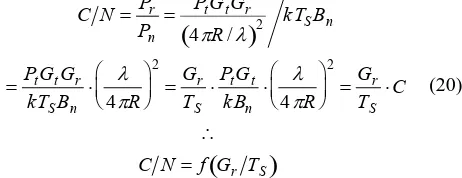
C.Figure of merit (G/T)

From equation (4) we have the power of the carrier signal at

the receive antenna as Pr. And from equation (16) we have the

noise power given by the Nyquist equation. Since the C/N ratio is the ratio of signal power to noise power, we have that:



C N Pr

P_n 

P_tG_tG_r

4R/





2 kTSBn

 PtGtGr

kT_SB_n 



4R

      2

Gr

T_S  PtGt

kB_n 



4R

      2

Gr

T_S C



C N  f G



r TS



(20)

Where C is constant for a given operational mode of the

satellite, thus C/N  G/T. The ratio Gr/Ts (or simply G/T) is

known as the Figure of Merit. It indicates the quality of a

receiving satellite earth system and has a unit [dB/K].



Example G:

An earth station has a diameter of 30 m, and an overall efficiency of 69%. It is used to receive a signal of 4150 MHz. At this frequency, the system noise temperature is 79 K when the antenna points at the satellite at an elevation angle of 28˚. a) What is the earth station G/T under these conditions? b) If heavy rain causes the sky temperature to increase so that the system noise temperature increases to 88 K what is the change in G/T value?

Solution

a) From equation(7) we have that



G_r 4A

2    

D        2

at 4.15106Hz;  c f 0.0723 m 

G_r0.69  30

0.0723       2 1,172,856.9

60.69 dB

b)



For T_s79 K



10log79



18.98 dBK GT 60.6918.9841,71 dB/K

If T_s increases to 88 K in heavy rain, then T_s88 K



10log88



19.44 dBK

GT





/_

60.6919.4441,25 dB/K

Change in G/T value





G/T



GT 



G T



/41.7141.25

0.46 dB/K



VI. SYSTEM AVAILABILITY

The availability of a satellite communication system is the ratio of the actual period of correct operation of the system to the required period of correct operation [3]. This availability depends not only on the reliability of the constituents of the system, but also on the probability of a successful launch, the replacement time and the number of operational and back-up satellites (in orbit and on the ground). Availability of the earth stations depends not only on their reliability but also on their maintainability. For the satellite, availability depends only on reliability since maintenance is not envisaged with current techniques. Availability A is defined as given in equation (21).



A ROT - DT

ROT (21)

Where ROT and DT – Required Operational Time and Down Time respectively.

ROT is the period of time for which the system is required to be in active operational regime, while DT is the cumulative amount of time the system is out of order within the required

operational time. To provide a given system availability A for

a given required time L, it is necessary to determine the

number of satellites to be launched during the required time L.

This number will affect the cost of the service. The required

number of satellites N and the availability A of the system will

be evaluated for two typical cases for which Tr is the time

required to replace a satellite in orbit and P is the probability

of a successful launch.

A. No backup Satellite in Orbit

For this case, the number of satellites to be launched is given by equation (22).

110904-3232 IJECS-IJENS © August 2011 IJENS

Where L – ROT [years]; P – Probability of success of each

launch; T – mean time to failure (MTTF); U – Maximum

lifespan of satellite.

If it is assumed that satellites close to their end of maximum

lifetime U are replaced soon enough so that, even in the case

of a launch failure, another launch can be attempted in time, the mean unavailability (breakdown) rate is:



B



t

r

P



T

(23)

Where tr – time required for each replacement and the availability A = 1- B of the system is thus:



A



1



t

r

P



T

(24)

B. Back–up Satellite in Orbit

By assuming, pessimistically but wisely, that a back-up satellite has a failure rate of l and a maximum lifetime U equal to that of an active satellite, it becomes necessary to launch twice as many satellites during L years as in the previous case reflected in equation (22):



N



2

L





P



T



1



e

U T











(25)

Taking account of the fact that tr/T is a small value, the

availability of the system expressed in equation (22) becomes:

VII. LINK BUDGET

The link budget determines the antenna size to deploy, power requirements, link availability, bit error rate, as well as the overall customer satisfaction with the satellite service. A link budget is a tabular method for evaluating the power received and the noise ratio in a radio link [2]. It simplifies C/N ratio calculations

The link budget must be calculated for an individual transponder, and must be recalculated for each of the individual links. Table II below shows a typical link budget for a C band downlink connection using a global beam GEO satellite and a 9m earth station antenna. Link budgets are usually calculated for a worst-case scenario, the one in which the link will have the lowest C/N ratio or lowest tolerable availability.

TABLE II

C–BAND GEOSATELLITE LINK BUDGET IN CLEAR AIR

C – band satellite parameters

Transponder saturated output power 20 W Antenna gain on axis 20 dB Transponder bandwidth 36 MHz Downlink frequency band 3.7 – 4.2 GHz Signal FM – TV analogue signal

FM – TV signal bandwidth 30 MHz Minimum permitted overall C/N in receiver 9.5 dB Receiving C – band earth station

Downlink frequency 4 GHz Antenna gain on axis at 4GHz 49.7 dB Receiver IF bandwidth 27 MHz Receiving system noise temperature 75 K Downlink power budget

Pt – satellite transponder output power, 20 W 13 dB Bo – transponder output backoff -2dB Gt – satellite antenna gain, on axis 20 dB Gr – earth station antenna gain 49.7 dB LP – free space path loss at 4GHz -196.5 dB Lant = edge of beam loss for satellite antenna -3 dB La = clear air atmospheric -0.2 dB Lm = other losses -0.5dB Pr = received power at earth station -119.5 dBW

Downlink noise power budget in clear air

k = Boltzmann’s constant -228.6 dBW/K/Hz TS = system noise temperature, 75 K 18.8 dBK Bn = noise bandwidth 27 MHz 74.3 dBHz

N = receiver noise power -135.5 dBW

C/N ratio in receiver in clear air

C/N =Pr – N = -119.5 – (-135.5) 16.0 dB

VIII. SATELLITE LINK DESIGN METHODOLOGY

The design methodology for a one-way satellite

communication link can be summarized into the following steps. The return link follows the same procedure.

Methodology

Step 1.Frequency band determination.

Step 2.Satellite communication parameters determination.

Make informed guesses for unknown values.

Step 3.Earth station parameter determination; both uplink and

downlink.

Step 4.Establish uplink budget and a transponder noise power

budget to find (C/N)up in the transponder

Step 5.Determine transponder output power from its gain or

output backoff.

Step 6.Establish a downlink power and noise budget for the

receiving earth station

Step 7.Calculate (C/N)down and (C/N)0 for a station at the

outermost contour of the satellite footprint.

Step 8.Calculate SNR/BER in the baseband channel.

Step 9.Determine the link margin.

Step 10. Do a comparative analysis of the result vis-à-vis the

specification requirements.

Step 11. Tweak system parameters to obtain acceptable

(C/N)0 /SNR/BER values.

Step 12. Propagation condition determination.

Step 14. Redesign system by changing some parameters if the link margins are inadequate.

Step 15. Are gotten parameters reasonable? Is design

financially feasible?

Step 16. If YES on both counts in step 15, then satellite link

design is successful – Stop.

Step 17. If NO on either (or both) counts in step 15, then

satellite link design is unsuccessful – Go to step 1.

IX. CONCLUSION

A number of factors have to be taken into consideration in the design of a robust satellite link. We have presented the most salient of these factors and examined how they are interrelated vis-à-vis satellite link design for the provision of optimal service availability. The transmitted and received power of the link between the satellite and earth stations must be accounted for, losses due to the link and communication equipments

must be taken into consideration et cetera. The link ratios,

which include carrier–to–noise and Bit error rate are good indicators of the feasibility of the system design. The system availability is another factor of high interest, and must therefore be taken into account. Frequency re – use enhances the capacity of the satellite, which makes it a vital element for optimizing the link. A sample link budget was outlined to illustrate the process. We have summarized in the satellite link design methodology the most salient points necessary for achieving a robust satellite link design with desired characteristics.

REFERENCES

[1] Dennis Roddy, “ Satellite Communications”, 3rd edition, McGraw Hill, USA, 2001, ISBN: 0-07-120240-4

[2] Timothy Pratt et al., “Satellite Communications “Copyright©2003, ISBN: 9814-12-684-5

[3] Gerard Maral and Michel Bousquet, “ Satellite Communication Systems”, 5th edition, John Wiley, UK, 2002

[4] International Telecommunications Union, “Handbook on satellite communications”, 3rd edition, April, 2002, ISBN: 978-0-471-22189-0. [5] J. A. Pecar, “The New McGraw-Hill Telecom Factbbok”, McGraw-Hill,