Mathematical Description of the Implementation of
the Adaptive Newton-Raphson Method in
Compositional Porous Media Flow
Akmal Aulia
∗, Noaman El-Khatib
∗∗
Enhanced Oil Recovery Centre
Department of Geoscience and Petroleum Engineering
Universiti Teknologi PETRONAS, Bandar Seri Iskandar, 31750 Tronoh, Perak, Malaysia
Abstract—Models for multiphase-multicomponent flow in porous media are described in systems of PDEs. Solving them using finite difference discretization method can be of three ways; explicit, semi-implicit, and fully implicit. In this study, we present the implementation of an adaptive Newton-Raphson method in the context of IMPECS (Implicit Pressures Explicit Concentrations and Saturations) method of solution.
Index Terms—Reservoir Modeling, Adaptive Newton-Raphson, Compositional Model, Fluid Flow in Porous Media, Finite Dif-ference, Conjugate Gradient
I. INTRODUCTION
T
HIS paper is an extension of the authors’ previous work [1].As an oil field matures, EOR (enhanced oil recovery) methods become necessary in order to boost the oil produc-tion. Chemical EOR, for example, is a method in which a reservoir / porous media is injected by one or more chemicals such as polymer, surfactant, and alkali in order to achieve mobility control, IFT (oil-water interfacial tension), and pH conditioning, respectively. These chemicals are considered to be expensive, and therefore a careful study needs to be carried out prior to executing a chemical EOR project.
Reservoir simulation has played a very important role in the feasibility analysis of surfactant injection projects. Mathematical models have been developed for single phase flow, dual phase flow, and a more generalized multiphase-multicomponent flow. The latest model development appropri-ate for simulating surfactant flooding is the compositional flow model, where transport of multicomponent in a multiphase flow environment is considered.
Compositional simulators enabled one to study the sitional dynamics inside the reservoirs. Knowing the compo-sitions of oil, water, chemicals, salts, and others in a given reservoir is important in determining its behavior; the study of phase behavior is essential in tuning the optimal chemical injection configurations for oil recovery improvement.
Progress have been made in the development of compo-sitional flow simulators for the past 30 to 40 years. One of the earlier works in compositional simulation was by Nolen (1973). His contribution was a 3-dimensional compositional simulator. Here, the simulator provides consistent and ac-curate fluid properties such as density, viscosity, k-values
(flash calculation). The work was compared with experimental approaches. Method used in eliminating numerical dispersions was shown [2].
The work of Pope and Nelson (1978) incorporates quite a number of more factors including adsorption and dispersion, and also the electrolyte and surfactant concentrations, the polymer viscosity, fractional flow, cation exchange, chemical slug size, and the transport of polymer in their compositional simulator [4]. This study is one of the very first in depth anal-ysis on the effects of many mechanisms in a one dimensional scope.
A year later, Coats (1979) compiled a 3D implicit com-positional simulator using the Equation of State (EOS). The EOS is used in order to perform computations on phase equilibrium and property calculations, due to its consistent and smooth nature nearby the critical point. His simulator applied an implicit method thus enhancing its reliability as well as efficiency [5].
Another work was introduced by Porcelli and Bidner (1994) in 3 component, 2 phase, compositional simulator. Here, many factors were included in the modeling; ultralow IFT, capil-lary pressure, component partition, dispersion, and adsorption. They used an explicit and iterative technique in solving the 1D compositional model. The main objective of their study is to analyze the effects of the factors mentioned on the compositional dynamics and oil recovery [6].
In this study, we would like to introduce the adaptive Newton-Raphson method for solving the overall compositions, saturations, and phase compositions. Here, we presented the analytical derivations and numerical technique in order to enable such adaptivity of the Newton-Raphson algorithm. The mathematical models for the compositional flow are also presented in this paper.
II. MATHEMATICALBUILDINGBLOCKS
Darcy’s Equation. Given a fluid flow system, we can
write the generalized energy balance from a Lagrangian (point particle) flow perspective as follow [9],
∂q−∂w= ∂u 2
2gc
+ g
gc
∂z+ ¯V dP+∂ξ (1) where q is the heat entering the system (per unit mass); w is work performed by the system (also, per unit mass); u is the velocity; z is the relative elevation; g is the gravitational acceleration,gc is the gravitational constant;V¯ is the specific
volume;Pis the fluid pressure;ξis the lost work. It is essential to note that the terms ∂u2g2
c and g
gc∂z represents kinetic and
potential energy, respectively.
The change of lost work ξ can also be described in terms of the change of entropy such that,
∂ξ=T ∂S (2)
which reveals that lost work causes disturbance that leads the system away from equilibrium, thus increasing the entropy of the system. This fact is just another description of the second law of thermodynamics.
The fluid system’s lost work can also be described a friction factor relationship [9],
∂ξ=f u
2
2gcD
∂x (3)
where f is the friction factor; x is the distance in the flow direction;Dis the characteristic dimension of the flow system. The variable D can be the particle diameter, given a packed bed where a particular flow may penetrates; this can be a good representation for modeling fluid flow in porous media.
Friction factor f can be defined according to the flow regime, i.e. laminar or turbulent, as a function of the Reynolds number,
f = c
Re (4)
where c is a constant for the flow configuration, and the Reynolds number Re expression reads,
Re=Duρ
µ (5)
whereρandµare the fluid density and viscosity, respectively. Substituting the previous relation to the original friction factor relationship yields to,
∂ξ= Duρc
µ
· u
2
2gcD
∂x (6)
Solving the above equation for the fluid velocity uyields, u=2gcD
2
c ·
1
µ·ρ ∂ξ
∂x (7)
Defining a new variableK such that, K= 2gcD
2
c (8)
we can rewrite the velocity expression as, u=K
µρ ∂ξ
∂x (9)
Furthermore, we can substitute the lost work termdξin the previous equation by solving the generalized energy balance equation (Eq. 1) for dξ,
∂ξ=∂q−∂w−du 2
2gc
− g
gc
∂z−V ∂P¯ (10) which yields the velocity expression,
u= K
µρ
dq−dw−gg c∂z−
¯
V ∂P
∂x (11)
It is important to note that in porous media flow, the kinetic effects can be neglected.
Assuming an isolated system (i.e. no heat and mass ex-change), and having the specific volumeV¯ = 1ρ, therefore
u = K
µρ −
1
ρ∂P
∂x −
g gc∂z
∂x
!
= −K
µ ∂P
∂x + ρgg
c∂z
∂x
!
(12)
The termρ
g gc∂z
∂x can be eliminated for a horizontal flow system,
thus enabling us to obtain the Darcy’s law for horizontal flow as,
u=−K
µ ∂P
∂x (13)
Eq. 13 is also known as the Darcy’s law.
The Darcy’s law can be used to describe the velocity of each phases. For some phase l ∈ L = {o, a}, given the mobility relation λl = Kkrl
µl , we can express the phase velocities as
follow,
ul = −λl∂P
l
∂x (14)
u = uo+ua (15)
Here,u andPl are regarded as the total velocity and the lth
phase pressure, respectively.
Continuity Equations. We can describe the dynamics of
compositions of components in the reservoir by utilizing the continuity equations. The models presented here refers to the work of Bidner and Porcelli (2002) [10]. Let C be the set of all components such that C = {p, w, s}; p=oil, w=water, s=surfactant. Also, letLbe the set of all phases such thatL=
{a, o}; a=aqueous, o=oleic. ∀i ∈ C, the continuity equation reads,
φ∂Ci ∂t +
∂ ∂x
X
l∈L
cliul− ∂
∂x
X
l∈L
SlKl∂cli
∂x =− ∂Γi
∂t (16) Here, Ci is the overall concentration of the ith component;
cl
is the Darcy’s velocity of the lth phase; Kl is the dispersion
coefficient ; and Γi is the ratio describing the adsorption of
the ith component by the porous media.
Overall Continuity Equation. Summing the continuity
equation over all of the components yields the overall con-tinuity equation,
∂ ∂x
λ∂P
a
∂x
= ∂
∂t
X
i∈C
Γi
!
− ∂
∂x
λo∂PC ∂x
(17)
Here, PC is regarded as the capillary pressure, which can
be given by the difference of the pressures between the two coexisting phases,
PC=Po−Pa (18)
The overall continuity equation (Eq. 17) is also known as the pressure equation, since utilizing it enables one to solve for the pressure distribution throughout the entire flow system. Here, using Eq. 15, the total velocity ucan be rewritten as,
u=−λ∂P
a
∂x −λ
o∂PC
∂x (19)
Adsorption. The irreversible adsorption term Γi can be
described by the Langmuir expression [11],
Γi=
a1cli
1 +a2cli
, ∂c
l i
∂t ≥0 (20) ∂Γi
∂t = 0,
∂cli
∂t <0 (21) Eq. 20,21 model the irreversibility of the adsorption process. Assuming incompressible fluids on the media, we can write the volume fractions of component son phasel as [11],
cls= max(c
a s, c
o
s) (22)
Dispersion.Molecular diffusion and longitudinal dispersion
can be described by [3] [12],
K
Dm
= 1
F φ+ 1.75 U dp
Do
(23)
whereKis the longitudinal dispersion coeffiicient;Dmis the
molecular diffusion coefficient; F is the formation electrical resistivity factor;φis the fractional porosity;U is the average velocity; and dp is the particle diameter.
Auxilary Relations. The essence of compositional
model-ing is to acknowledge the effects of compositions on the fluid properties such as the oil-water IFT (interfacial tension), rela-tive permeabilities, residual saturations, and phase viscosities. Many of these auxilary relations are intertwined with each other, thus demanding a special way in order to solve the continuity equations, as well as the overall continuity equation. The relative permeabilites in this study can be described by the following equations [10],
klr=krl0
Sl−Slr
1−Slr−Sl0r
el
; l6=l0 (24)
kl0
r andel can be obtained from,
krl0 = (1−krl0H) 1− S l0r
Sl0rH
!
+krl0H (25)
el = (1−elH) 1− S l0r
Sl0rH
!
+elH (26)
Here,k0
r andel are the endpoint and curvature of the relative
permeability as a function of phase saturations, respectively. In similar way,kr0HandelHare the endpoint and curvature of the relative permeability as a function of phase saturations, given no surfactant injected; the symbolH reflects the parameter at high IFT system.Slr is the phase residual saturation.
Assuming a Type II(-) phase behavior condition, the IFT for a surfactant flooded system can be expressed depending upon the ratio c
a p ca
s. For cap ca
s ≤
1, the IFT expression reads [10],
logσ= logF+
1−c
a p
ca s
logσH+ G1
G2+ 1
(27)
As for c
a p ca s
>1, the IFT can be given by,
logσ= logF+ G1
1 +cap
ca sG2
(28)
where G1 and G2 are both constant parameters, and F is
a factor that reduces the IFT to null at the plait point, and expressed as a function of composition,
F =1−e
−pP i∈C(c
o i−cai)2
1−e−√2 (29)
The symbol σH represents the oil-water IFT without having chemicals involved.
Phase viscosities dependency upon compositions of compo-nents can be described by the following,
µl=clwµaHeα1(clp+cls)+cl pµ
oHeα1(clw+cls)
+clsα3eα2(c
l
w+clp) (30)
The residual saturations of each phases can be determined from,
Slr
SlrH =
1, if Nc<10(1/T
l i)−T2l;
Tl
1[log(Nc) +T2l], if 10(1/T
l i)−T
l
2≤Nc≤10−T l 2 ;
0, if Nc>10−T
l 2
Here,Ncis the dimensionless capillary number.T1landT2lare
the trapping numbers, and typically given as constants.
Restriction Relations.Restriction relations are also
These relations can expressed in the following, Ci =
X
l∈L
Slcli (31) X
i∈C
cli = 1 (32)
X
l∈L
Sl = 1 (33)
X
i∈C
Ci = 1 (34)
III. FINITEDIFFERENCEDISCRETIZATIONS
Setting up the finite difference method to the continuity equation (Eq. 16) for m gridblocks, n timesteps, and k iterations yields,
φ
4t(C
n+1
i −C n i )m
+ 1
4x
X
l
(ul,nm+1,k+1c
l,n+1,k i,m −u
l,n+1,k+1
m−1 c
l,n+1,k i,m−1 )
− 1
4x2
X
l
[(SlKl)
m+1 2(c
l
i,m+1−c
j i,m)
−(SlKl)m−1 2(c
l i,m−c
l i,m−1)]
n+1,k
=−(Γ
n+1
i −Γ n i)km
4t (35)
As you can see, Eq. 35 is discretized using the explicit finite difference scheme.
Similarly, we can apply the finite difference to the overall continuity equation (Eq. 4) to give,
λnm+1+1,k(Pma+1−Pma)n+1,k+1
−λnm+1,k(Pma −Pma−1)n+1,k+1
=4x
2
4t (Γ
n+1,k
−Γn)−[λom+1(PCm+1−PCm)
−λom(PCm−PCm−1)]
n+1,k (36)
The implicitness shown in Eq. 36 requires one to solve for a matrix-vector system (see Section IV).
The Darcy equations for all phases can be treated using the central difference scheme as follow,
(u)nm+1,k+1=−λnm+1,k
Pa
m+1−Pma−1
24x
n+1,k+1
−(λo)nm+1,k
P
Cm+1−PCm−1
24x
n+1,k (37) The aqueous phase Darcy velocity can also be expressed the central difference scheme,
(ua)nm+1,k+1=−(λa)nm+1,k
Pa
m+1−Pma−1
24x
n+1,k+1 (38)
Initial and Boundary Condition.The initial and boundary
conditions for solving the above finite difference equations will be categorized into three ranges of time; at initial time t=t0, at some finite span of time0≤t < tswhen surfactant
injection occurs, and post injection time regiont > ts.
At t = 0, we can define the initial condition as the following [10],
0≤x≤L; Cs= 0; Cp=SorH; Pa=PIN (39)
During surfactant injection, the initial condition is defined as,
x= 0; Cs=CsIN; Cp =CpIN (40)
The following conditions are also used,
t > ts; Cs= 0; Cp= 0 (41)
x= 0; t >0; −λ∂P
a
∂x =u
IN
(42) x=L; t >0; Pa=POUT (43)
IV. IMPECSAS AMETHOD OFSOLUTION
As mentioned previously, the IMPECS method implies the use of implicit finite difference for solving pressure distri-bution, and explicit finite difference for solving the overall concentrations and saturations.
The description of steps for all gridblocks in a given time step is shown by the following IMPECS algo-rithm [10] [11]:
forerror≤TOLdo
STEP 1: CalculatePa via Eq. 36
STEP 2: CalculatePo via Eq. 18
STEP 3: Calculateu, ua, uo via Eq. 15, 37, 38
STEP 4: CalculateCc, Cp via Eq. 35
STEP 5: CalculateCw, c j i, S
j via Eq. 31-34
STEP 6: Evaluate error of the current iteration
end for
where the error can be evaluated ∀i∈ {p, c},
error=
M X
m−1
|(Ci)km+1−(Ci)km| (44)
STEP 1 involves calculating the pressure distribution by solving the matrix-vector system due to the implicit scheme used. Therefore, the conjugate gradient (CG) algorithm is needed to solve such system [13]. Mathematically speaking, this system can be described as somex∈Rgiven some linear transformationg:x→b that reads,
Ax=b (45)
Let x0 as the initial guess vector. Thus, the CG algorithm
can be written as follows,
r0 = b−Ax0 (46)
zo = C−1r0 (47)
The next iterations, having an iteration counterk∈Z+, are
defined as the following: αk =
zT krk
dT kAdk
(49)
xk+1 = xk+αkdk (50)
rk+1 = rk−αkAdk (51)
zk+1 = C−1rk+1 (52)
βk+1 =
zkT+1rk+1
zT k
(53)
dk+1 = zk+1+βk+1dk (54)
At times, the matrix A can be ill-conditioned, that is converging to the true solutionx∗ can be difficult or perhaps impossible. Therefore, a preconditioner can be used in order to avoid such problem [13]. One of the well-known precon-ditioner is the Jacobi preconprecon-ditioner. This method basically takes the diagonal of the matrix Aand use it to define a new matrix C such that,
Cij =
Aii, ifi=j
0, otherwise.
The calculations for STEP 2 and STEP 3 are straightforward by applying Eq. 15, 18, 37, and 38. Th results from these 2 steps will be used in STEP 4 to solve for the overall concentrations explicitly. Then, algebraic manipulations of the restriction relations (Eq. 31-34) can help to solve the rest of the variables. In the next section, we shall see how the adaptive Newton-Raphson method can be used in order to conduct STEP 5 with several defined constraints.
V. IMPLEMENTATION OF THEADAPTIVE
NEWTON-RAPHSONMETHOD
The ratios of phase compositions (phase behavior relations) mentioned previously can be represented by the following,
Lapc =
ca p
ca c
(55)
Lowc = c
o w
co c
(56)
Kc =
co c
ca c
(57) La
pc, Lowc, and Kc are the swelling parameter, solubilization
parameter, and equilibrium ratio between the two phases, respectively.
Recall Eq. 31, one can therefore write the previous restric-tion relarestric-tion for the chemical component by using the phase behavior relations as,
Cc = X
l∈L
Sjclc
= Sacac +Sococ
= Sacac + (1−Sa)Kccac (58)
It is important to note here that the intention is to set up a Newton-Raphson algorithm for two-dimensional vectors, therefore we attempt a solvable matrix-vector system that comprises 2 equations and 2 unknowns, namely Sa and ca
c.
Eq. 31 can also be written for the petroleum component as follow,
Cp = Sacap+S oco
p
= SaLapccac + (1−Sa)(1−coc−cow)
= SaLapccac + (1−Sa)(1−Kccac −L
o wcc
o c)
= SaLapccac + (1−Sa)(1−Kccac −LwcoKccac)
= SaLapccac + (1−Sa)(1−Kccac(1 +L
o wc))
(59) At this stage, Eq. 58 and Eq. 59 can be solve using the Newton-Raphson algorithm by forming the following equa-tions,
f1(Sa, cac) = S aca
c+ (1−S a)K
ccac −Cc (60)
f2(Sa, cac) = S aLa
pcc a
c + (1−S a)
(1−Kccac(1 +L
o
wc))−Cp (61)
Notice that the variableCcandCpcan be calculated by solving
the continuity equations explicitly, as have been shown in Section II and III.
Letting some iteration counter k ∈ Z+, the
Newton-Raphson equation for 2 dimension vectors (2 equations, 2 unknowns) reads,
− →x
k+1=−→xk−J−1 − →
fk (62)
where,
− →x
k=
Sa
cac
k
− →
fk = "
x1
x2
#
k
=
"
f1(Sa, cac)
f2(Sa, cac) #
k
and,
J=
∂f1
∂x1
∂f1
∂x2
∂f2
∂x1
∂f2
∂x2
k
where,
∂f1
∂x1
= cac(1−Kc) (63)
∂f1
∂x2
= Sa(1−Kc) +Kc (64)
∂f2
∂x1
= cac(Lapc+Kc(1 +Lowc))−1 (65)
∂f2
∂x2
= Sa(Lapc+Kc(1 +Lowc))
The restriction relations require the solution of the system of equations to satisfy 0 ≤ Sa ≤ 1 and 0 ≤ ca
c ≤ 1.
Moreover, it should also be noted that the inequality Sar ≤
Sa ≤(1−Sor)must hold. Therefore, it is important to enable
the algorithm to adapt to the constraint mentioned previously. Schematic representation adaptive Newton-Raphson for the case(Sa)
k+1< Sar is shown in Figure 1.
!"
#$%& !
" #& !"
#$%& !"'
& %(!"'&
Fig. 1. Description of the Adaptive Newton-Raphson.
In mathematical terms, we can describe the adaptivity of the Newton-Raphson for Sa as follows.
(Sa)k+1=
(Sa)
k+Sar
2 , if(S
a)
k+1< Sar
(Sa)k+ (1−Sor)
2 , if(S
a)
k+1>(1−Sor)
(Sa)
k+1, otherwise.
Similarly, for ca c reads,
(cac)k+1=
(ca
c)k+ 0
2 , if(c
a
c)k+1<0
(cac)k+ 1
2 , if(c
a
c)k+1>1
(ca
c)k+1, otherwise.
VI. RESULTS ANDDISCUSSION
The discretized models were implemented in FORTRAN, utilizing the latest GNU license GFortran compiler. Here, adsorption, dispersion, and capillary pressure are neglected.
The developed simulator comprised of several subroutines. The subroutine dependencies is shown in Figure 2.
!"#$%&' ()*+,-'
./0123'
4"5/6#7'*325/$8#9/$28' ,/$:;<"=2'>3"8#2$=' ?8"@912'A2B=/$7C"@D./$'
Fig. 2. Subroutine Dependencies.
Here, the main program executes the IMPECS at a single time step. The IMPECS solver performs the computation of all variables; primarily pressures, overall concentrations, phase
compositions, and saturations. Since the pressures were solved implicitly, the resulting matrix-vector system needs to be solve using the preconditioned conjugate gradient subroutine. As said in the previous section, once the overall concentrations are solved in the IMPECS, the adaptive Newton-Raphson subroutine are used in order to solve the 2 variables, namely ca
c andSa.
Assigned values for the input parameters to the simulator are shown in Table I. It is essential to note that the metric unit system was used thoroughly in this study.
TABLE I
COMPOSITIONALSIMULATOR’SINPUTPARAMETERS
Parameter Assigned Value Units Description
uIN 10−4 cm/s input flowrate
SorH,SarH 0.35 res. sat. at high IFT
PIN,POUT 1 atm endpoint Pressures
φ 0.24 porosity
CIN
s 0.1 overall surfactant conc.
CIN
p 0 overall oil conc.
L 100 cm core (porous media) length
K 0.5 Darcy permeability
ko0H
r ,kar0H 1, 0.2 Rel. Permeability at high IFT
µoH,µaH 5, 1 cP phase viscosities
Several results were obtained. The aqueous phase pressure distribution is displayed in Figure 3.
0.99 1 1.01 1.02 1.03 1.04 1.05 1.06 1.07 1.08 1.09 1.1
1 2 3 4 5
n=1 n=2 n=3
Fig. 3. Aqueous phase pressures across grid at different timesteps.
Here, the aqueous phase pressure was assumed constant at the beginning. At the next two timesteps(n= 2 and n= 3), surfactant injection is applied having constant velocity. Figure 2 shows that as time passes, the aqueous phase pressure increases particularly at locations near to the injection point.
The distribution of the surfactant content in the aqueous phase across grid is shown in Figure 4. Here, the surfactant can be seen to increase at grid no. 2, whilst at other grids the surfactant content is slowly increasing as well.
The phenomena in Figure 4 can yield to a conclusion such that the surfactant tends to exceedingly accumulate near the injection point maybe due to the neglected dispersion term.
0 0.1 0.2 0.3 0.4 0.5 0.6 0.7 0.8 0.9 1
1 2 3 4 5
n=1 n=2 n=3
Fig. 4. Surfactant phase composition (aqueous phase) across grid at different timesteps.
0 0.1 0.2 0.3 0.4 0.5 0.6 0.7 0.8 0.9 1
1 2 3 4 5
n=1 n=2 n=3
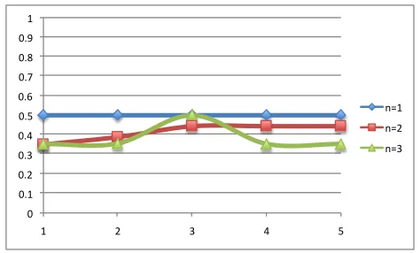
Fig. 5. Surfactant phase composition (oleic phase) across grid at different timesteps.
smaller that that of the aqueous phase, which indicates that the surfactant tends to solubilize in water. This is consistent by our original assumption that the porous media flow system is Type II negative (low salinity).
0 0.1 0.2 0.3 0.4 0.5 0.6 0.7 0.8 0.9 1
1 2 3 4 5
n=1 n=2 n=3
Fig. 6. Aqueous phase saturation across grid at different timesteps.
From Figure 6 and Figure 7, we can see the saturation profile of both phases. Here, the adaptive Newton-Raphson setups have successfully kept the Sa andCca values conform
to the piecewise restriction relations described in the previous section.
Fig. 7. Oleic phase saturation across grid at different timesteps.
VII. CONCLUSION
In this study we presented the technique for implement-ing the adaptive Newton-Raphson method for compositional model describing multiphase-multicomponent flow in porous media, in order to ensure satisfactory results which comply with the defined constraints, i.e. restriction relations.
ACKNOWLEDGMENT
The authors would like to thank the University of Technol-ogy PETRONAS for the financial support. The authors would also like to thank Prof. Dr. Birol Demiral (Head of the EOR Centre, University of Technology PETRONAS) for providing us with excellent feedbacks and computing facilities.
REFERENCES
[1] Akmal Aulia, Noaman El-Khatib, ”Mathematical Modeling of Adsorption and Dispersion in Chemical Flood EOS Compositional Flow,”, paper presented at the International Conference in Integrated Petroleum Engi-neering and Geosciences (ICIPEG), Kuala Lumpur, June 15-17, 2010. [2] J. S. Nolen, ”Numerical Simulation of Compositional Phenomena in
Petroleum Reservoirs,” paper SPE of AIME 4274, page 1-16, 1973. [3] L. W. Lake,Enhanced Oil Recovery, Prentice Hall, New Jersey, 1989. [4] G. A. Pope and R. C. Nelson, ”A Chemical Flooding Compositional
Simulator,” paper SPE of AIME 6725, page 339-354, 1978.
[5] Keith H. Coats, ”An Equation of State Compositional Model,” paper SPE 8284, Dallas, Texas, September 1979.
[6] P. C. Porcelli and M. S. Bidner, ”Simulation and Transport Phenomena of a Ternary Two-Phase Flow”, Transport in Porous Media, pages 101-122, 1994.
[7] H. Kazemi, C. R. Vestal, and G. Deane Shank, ”An Efficient Multicom-ponent Numerical Simulator,” paper SPE of AIME, October, 1978, pages 355-367.
[8] Fernando Rodriguez, Agustin Galindo-Nava and Javier Guzman, ”A General Formulation for Compositional Reservoir Simulation”, SPE International Conference and Exhibition of Mexico held in Veracruz, Mexico, 10-13 October 1994.
[9] E. J. Hoffman,Unsteady-State Fluid Flow: Analysis and Applications to Petroleum Reservoir Behavior, Elsevier Science, August 1999. [10] M. Susana Bidner, Gabriela B. Savioli, ”On the Numerical Modeling
for Surfactant Flooding of Oil Reservoirs,” Mec´anica Computacional, vol. 21, pages 566-585, Santa Fe-Paran´a, Argentina, October 2002. [11] M. S. Bidner, P. C. Porcelli, ”Influence of Phase Behavior on Chemical
Flood Transport Phenomena,” Transport in Porous Media, vol. 24, pages 247-273, 1996.
[12] T. K. Perkins, O.C. Johnston, ”A Review of Diffusion and Dispersion in Porous Media,” paper SPE 480, Jan. 15, 1963.
[13] Jorge Nocedal and Stephen J. Wright, Numerical Optimization, Springer, 1999.
Akmal Aulia is currently a Petroleum Engineer-ing Ph.D. Candidate at the Enhanced Oil Recov-ery Centre, University of Technology PETRONAS, Malaysia. His current research interests are in the numerical simulations of Chemical EOR and ap-plications of data mining in oil/gas. He holds two M.S. degrees; Information Technology from Heriot-Watt University (UK), and Computational Math-ematics from San Diego State University (USA). He completed his bachelor’s degree in Chemical Engineering at the Institute of Technology Bandung (Indonesia). Akmal Aulia has 6 years experience in scientific software development in the areas of oil/gas, bioinformatics, and remote sensing.