Forestry & Natural-Resource Sciences Last Correction: Aug. 15, 2013
TRENDS AND PROJECTIONS FROM ANNUAL FOREST
INVENTORY PLOTS AND COARSENED EXACT MATCHING
Paul C Van Deusen
1, Francis A Roesch
2,
1
National Council for Air and Stream Improvement, Mount Washington, MA, USA
2
USDA Forest Service, Southern Research Station, Asheville, NC, USA
Abstract.The coarsened exact matching (CEM) method is used to match annual forest inventory plots awaiting remeasurement with plots that have already been remeasured. This results in a model-free approach for short term inventory projections. CEM has many desirable properties relative to other matching methods and is easy to apply within a SQL database. The combination of short term projections with a 3 or 5 year moving window is suggested for providing trend estimates that include the current year and a few years into the future. The default projection represents business as usual. A method to bias the plot matching to generate desired scenarios is also developed. These ideas and methods are demonstrated with several applications to forest inventory data. Scenarios are generated where increasing future harvest levels are stochastically controlled to demonstrate this capability with operational data.
Keywords: Forest inventory, Moving average, Inventory projection, FIA data
1
Introduction
The United States Department of Agriculture (USDA) Forest Service’s Forest Inventory and Analysis program (FIA) has implemented an annual inventory system in the USA that involves measuring a proportion of the plots every year in each state. The annual percentage of plots measured is nominally 20% in most eastern states and 10% elsewhere. The plots measured in the same year are said to be in the same panel. The number of years required to measure all plots in a state is called a cycle (Tab. 1). The set of the most recent measurements for all plots in a state is called the current evaluation group (EVALGRP). Therefore, the first EVALGRP for a state on a 5 year cycle is completed in year 5. Thereafter, a new EVALGRP is created each year by updating the measurements for the current panel.
A common way to obtain estimates for a state is to compute the mean for the variable of interest over all plots in the most recent EVALGRP. This estimator (Bechtold and Patterson , 2005; Reams and Van Deusen , 1999; Roesch et al. , 2003; Van Deusen , 1997) is often called a moving average (MA), since the average from one EVALGRP to the next changes as the current panel is updated.
One concern with this approach is that the aver-age of an EVALGRP does not represent a particular year, rather it represents some time point between when
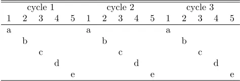
Table 1: FIA plots measured on 5 year cycles. The plots are placed into 5 panels labeled a,b,c,d and e. The same panel is measured during the same year within each cy-cle. All 5 year intervals have an associated EVALGRP that consists of the most current measurements for each panel. In practice, this idealized plan is not exactly fol-lowed.
cycle 1 cycle 2 cycle 3
1 2 3 4 5 1 2 3 4 5 1 2 3 4 5
a a a
b b b
c c c
d d d
e e e
the first measurements and the last measurements were taken for the EVALGRP. Clearly, a 5-year MA as de-fined by FIA, applied to the center of the period rather than the end of the period, is the 5-year moving win-dow (MW). It follows that methods developed for vari-ance estimation with the MA apply directly to the MW, so the MW requires no additional theoretical develop-ment. There is also no reason that estimates should be constrained to plots within an EVALGRP, which is an unnecessary limitation when looking at trends. For
ex-Copyright c2013 Publisher of theMathematical and Computational Forestry & Natural-Resource Sciences
ample, a 3-year MW is a very simple and useful way to look at trends in FIA data.
Users of FIA data would like estimates that corre-spond to the current year. They would also be interested in short term predictions for 5-10 years into the future. Short term projections of plots would be one way to satisfy both interests. For example, taking the moving window of a pseudo 5-year EVALGRP where years 4 and 5 are actually predictions, would result in an estimate for the current year. Likewise, the predicted years give an indication of what to expect in the near future.
There are also time series methods that could provide current estimates without using future predictions (Van Deusen , 1999), but time series methods are more com-plex than a MW or MA and don’t necessarily work with categorical data. Creating a pseudo EVALGRP where some of the panels are based on projections provides an approach for obtaining current estimates that fits in with existing procedures. If the projected data have all the features of real data, it can be analyzed with existing software. The objective here is to demonstrate how to use coarsened exact matching (CEM) to project annual forest inventory data to provide current estimates and short term projections.
2
Plot matching for plot projection
Plot matching methods have been suggested and used for projecting FIA plots in previous studies (Van Deusen , 1997, 2010; Wear , 2011). Those studies were seeking multi-decade projections, whereas the interest here is in short term projections that correspond to the number of years in an FIA measurement cycle. A method is pro-posed that requires fewer assumptions than the methods in these earlier studies, but it does require availability of remeasured plots. In general, these applications have been based on hot-deck methods (Sande , 1983) that seek matches from the large FIA data base (Woudenberg et al. , 2010).
The proposed method is based on a subject plot and a set of remeasured plots. Suppose the remeasured plots have measurements for times 1 and 2. The idea is to match the subject plot with remeasured plots that have similar time 1 characteristics. Then the time 2 measure-ments are used as projections for the subject plot. Call this the match then project (MTP) approach. Other applications of plot matching have used a project then match (PTM) approach, where some of the variables on the subject plot, like age and basal area, are projected and then matched with variables on other plots.
The PTM approach can be applied in states or re-gions where no remeasured plots are available. However, PTM requires that some variables be projected before the matching takes place. The MTP approach can only
be used if remeasured plots are available. The advantage of MTP is that no model based assumptions are required for the projection. If the subject plot is similar to the time 1 measurement on the matched plot, then the time 2 measurement is likely to be a good representation of a possible future state of the subject plot.
The MTP approach will tend to give projections that correspond to the cycle length, if the cycle length is rela-tively constant within the set of remeasured plots. Addi-tionally, the MTP method naturally provides a business as usual (BAU) projection. For example, harvest lev-els in the projected data will be consistent with harvest levels in the matched plots. Levels of insect damage, storm damage and fire will also reflect what influenced the years between time 1 and 2 measurements on the matched plots. A model based alternative for BAU pro-jections is possible (Fernandez and Astrup , 2012), but requires specific assumptions about various factors that have influenced recent trends.
A default BAU projection naturally results from the MTP method, but it is also possible to manipulate the matching process to deviate from BAU. After discussing the details of the matching process, a method to bias the matching to simulate desired scenarios is developed. The matching process and scenario generation are demon-strated with example applications.
2.1 Plot matching methods Matching procedures have been traditionally used to compare treated and control groups in observational studies. Although the treated and control analogy doesn’t directly apply here, our treatment group would be the plots that need to be projected and the remeasured plots would be the control group. Regardless of terminology, it is clear that there are 2 sets of plots, subject and remeasured, and there is a need to find remeasured matches for the subject plots. The main goal of matching is to find remeasured plots that were similar to the subject plot at time 1. Then the time 2 measurements can be used as projections for the subject plot. A subject plot with earlier measurements can also be placed in the pool of remeasured plots as a potential match for other subject plots.
co-variates has been eliminated. Unmatched comparisons with observational data could otherwise be dominated by differences inXbetween the 2 groups.
In practice, there is no guarantee that PS matching will reduce the bias in comparisons of the 2 groups. Proper application of the method requires careful check-ing of the results and iterative re-application. PS meth-ods and Mahalanobis matching are members of the equal percent bias reducing (EPBR) class (Iacus et al. , 2011a,b) which works on average, but does not guarantee bias reduction for any particular data set. In fact, King et al. (2011) found that PS matching often approx-imates random matching, and can degrade inferences relative to not matching at all. Iacus et al. (2011a) present a new monotonic imbalance (MIB) class that offers improved operational performance.
2.2 Coarsened exact matching CEM is a member of the MIB class that is used here, in part, because it is easily applied to large databases with SQL code. More significantly, CEM-based estimates have many desirable statistical properties (Iacus et al. , 2011a,b). It has been shown that CEM dominates commonly used matching methods (EPBR and others) as measured by its ability to reduce imbalance, model dependence, estimation er-ror, bias, variance, mean square erer-ror, and other criteria for a range of data sets (Iacus et al. , 2011a,b).
CEM is surprisingly easy to implement. Matching on continuous variables may involve rounding or cre-ating meaningful categories. Categorical variables can be used directly or after reducing the number of cate-gories. CEM allows the user to operate in the natural k-dimensional data space. PS matching or Mahalanobis distance matching create a transformed measure that has less intuitive appeal. As such, CEM maintains con-gruence between the data space and analysis space and does not violateThe Congruence Principle (Iacus et al. , 2011b).
CEM might be best explained by considering how to apply it to the problem at hand, i.e. matching sub-ject FIA plots with the time 1 state of a remeasured plot. This is a special instance of what are generally called hot-deck methods (Sande , 1983). The first deci-sion is whether to match on plots or conditions. Each mapped plot condition can represent a unique situa-tion, so it was decided to match conditions. Hence, the FIA variable that corresponds to condition propor-tion (CONDPROP) became the first matching criterion. Since CONDPROP ranges between 0 and 1 it needs to be coarsened. CONDPROP was put into 5 categories ranging from 0 to 4 by applying the following function,
C=round(round(CON DP ROP∗100)/25). The coars-ened value of CONDPROP, C, ensures that conditions get matched with other conditions of similar size. This
eliminates the need to make adjustments to the post-matched magnitude of the measurements. Post-match condition size adjustment would involve a number of de-cisions about how to reduce or increase the condition size. In particular, increasing the size could lead to prob-lems if a small condition contained a few unusual trees, like giant redwoods.
In addition to CONDPROP, the following variables were used in the matching process:
OWNGRPCD The owner group code was not initially coarsened. This indicates if the owner of the FIA plot is in one of four groups:
1. National Forest
2. Other Federal
3. State and local government
4. Private
OWNGRPCD is a coarsened version of OWNCD provided by FIA.
FORTYPCD The FIA forest type code was used with-out any coarsening. Hence, plot conditions had to be matched with conditions having the same FORTYPCD.
STDORGCD Matching was also done on uncoarsened stand origin code, which indicates if the condition originated naturally or from planting.
SITECLCD The other matching variable that was not initially coarsened was site productivity class code which indicates site growth potential and is ex-plained in more detail below.
STDAGE Stand age was coarsened into a 10, 20, 30, and 40 year age class for younger stands. Stands greater than 40 and less than 60 went into class 50. Stands greater than 60 and less than 80 went into class 70. Stands 80 or older went into class 80.
BA Basal area was coarsened into increments of 20 (square feet per acre) with the following function,
B=round(BA/20), which sets basal areas of 11-29 to 1, and basal areas of 190-210 to 10.
2.2.1 What to do with unmatched plots After the initial application of CEM, there will usually be some plot conditions that aren’t matched. As the name sug-gests, a subject plot condition can only be matched if there are time 1 values for remeasured plot condtions that exactly match all of its coarsened values. Either these unmatched conditions must be discarded from the analysis, or further coarsening must be applied. The ap-proach used here involved 3 iterations. Iteration 1 was to apply the CEM method described above. All success-fully matched subject plots are then set aside.
Iteration 2 seeks matches for the remaining subject plot conditions by further coarsening owner group, stand age, basal area and site productivity,
OWNGRPCD The National Forest and Other Fed-eral categories are combined. This results in the following 3 categories
1. Federal
2. State and local government
3. Private
STDAGE Stand age is coarsened into 3 categories.
1. ST DAGE <30
2. 30≤ST DAGE <80
3. ST DAGE≥80
BA Basal area is coarsened into 3 categories
1. BA <30
2. 30≤BA <120
3. BA≥120
SITECLCD Site productivity class code is coarsened into 3 categories
1. SIT ECLCD≤2
2. 3≤SIT ECLCD <5
3. SIT ECLCD≥5
The original SITECLCD consists of 7 levels of produc-tivity (Woudenberg et al. , 2010). It is a classification of forest land in terms of inherent capacity to grow crops of industrial wood. It is an estimate of the potential growth and is based on the culmination of mean annual increment of fully stocked natural stands,
1. 225+ ft3/ac/yr
2. 165-224 ft3/ac/yr
3. 120-164 ft3/ac/yr
4. 85-119 ft3/ac/yr
5. 50-84 ft3/ac/yr 6. 20-49 ft3/ac/yr
7. 0-19 ft3/ac/yr
A third and final CEM iteration is applied to sub-ject plot conditions that were not matched in the first 2 iterations. This involved further coarsening of OWN-GRPCD, STDAGE, BA and SITECLCD,
OWNGRPCD Owner group is eliminated entirely for this final attempt to match plots.
STDAGE Stand age is coarsened into 2 categories.
1. ST DAGE <40
2. ST DAGE≥40
BA Basal area is coarsened into 2 categories
1. BA <50
2. BA≥50
SITECLCD Site productivity class code is coarsened into 2 categories
1. SIT ECLCD≤3
2. SIT ECLCD >3
The few plot conditions that have no matches after the 3 CEM iterations are excluded from further anal-ysis. Increased coarsening for CEM will increase the potential for bias. However, bias due to coarsening one variable does not effect bias in other variables. This is an important property of the CEM method not enjoyed by other non-MIB methods such as propensity score match-ing (Iacus et al. , 2011a,b).
3
Biasing the matching process to
generate scenarios
The CEM process results in nearly all plot conditions having at least one match, and many will have multiple matches. The multiple matches could be used to im-plement multiple imputation (McRoberts , 2001; Reams and McCollum , 2000; Rubin , 1987; Van Deusen , 1997) if obtaining better variance estimates for BAU predic-tions is a primary interest. However, an important ob-jective here is to select from the multiple matches to control how the results will deviate from a BAU sce-nario.
assigning a uniform (0,1) random variate (rv) to each matched condition and then selecting the matched con-dition with the largest rv. Now we want to modify this approach to bias the selections toward matches that were subjected to certain events. Specifically, the event must be something that happened after the time 1 measure-ment and is recorded in the database.
The event could be storm damage, insect attack, har-vesting or any well defined occurrence. Sort the matches for subject condition i so the matches where the event occurred come first, Mi ={e1, e2, ..., O1, O2, ...}, where ej denotes a matched condition that experienced the event and Oj is a match where the event did not oc-cur. Letuandu0 represent draws from a uniform (0,1) distribution andrbe some small positive value. Suppose the followingrv vector corresponds toMi,
RVi = {u1+r, u2+r, ..., u01, u
0
2, ...} (1)
where the random variables for the event impacted matches have r added to them. Now select the con-dition from the matched setMithat corresponds to the largest value inRVi. This approach increases the prob-ability of selecting a match that experienced the event. The value of rdirectly controls how likely it is that an event impacted match is selected.
It is important to understand the influence ofrto con-trol the scenario generation process. There are 2 ways that an event impacted condition,ei, will be selected, so the overall probability of an event winning the selection can be broken into 2 parts,
Part 1 At least one of the random variates correspond-ing touj+r≥1 inRVi.
Part 2 Alluj+r≤1 but an event impacted match still wins.
Part 1 of the overall probability is equivalent to
P(At least oneuj+r≥1) = 1 − pn1e (2)
where there are ne event impacted matches and
p1 = P(u+r ≤ 1) = 1/(1 +r). This is 1 minus the probability that none of theuj+r≥1
Part 2 is
P(uj+r≤1 ∀j and an event match wins) = pn1e ne
N
(3) With this information it is possible to solve for r to control the probability of selecting an event impacted match. This is done relative to the probability of an event occurring in the BAU scenario, which is PB =
ne/N, where N is the total number of matches for a
particular set of subjects. The overall probability of se-lecting an event impacted match as a function of r is the sum of the 2 parts,
Pr = 1 − pn1e + p
ne
1 ne
N (4)
Now define a value,Q=Pr/PB, which defines a sce-nario. For example, if r is set so that Q= 1.5 then the selected matches will have an expected 50% increase in events relative to the BAU scenario. Finally, solve for r as a function of Q,
r(Q) =
1−ne
NQ
N
N−ne
−ne1
−1 (5)
Setting Q=1 results in r=0, which yields the BAU scenario. Values ofQ >1 will cause the event impacted matches to be selected at a higher rate than under the BAU scenario. However, equation (5) must be carefully applied. It is not sufficient to compute a singler-value for an entire state. The most accurate method is to com-pute a uniquer-value for each plot and condition based on its specific set of matches. A plot condition that has 10 possible matches where only 1 gets harvested needs a differentr-value than if 8 of the matches get harvested. This is controlled by theneandN parameters (eq 5).
4
Example applications
The CEM matching and projection method is demon-strated with two applications. The scenarios that are considered involve selecting more plots that will ex-perience harvesting than what would occur in a BAU scenario. In addition to BAU where Q=1, we evalu-ate Q=0.5 (reducing harvest by 50%), Q=1.5 (increas-ing harvest by 50%), andQ=2.0 (increasing harvest by 100%).
4.1 Application to Maine data The first applica-tion is to Maine FIA data for the 2006-2010 EVALGRP. The CEM algorithm is applied in 3 stages as described above. This results in projections for 2011-2015. There is actual data for 2011, which results in the 2011 moving window consisting of actual data for 2010 and 2011 and projected data for 2012. The gross-growth over harvest-removals ratio (G/R) is displayed (Tab. 2) for increasing harvest rate scenarios. G/R>1 for all years from 2005-2010 and for the BAU and +50% projections. This sug-gests that Maine forests are being sustainably managed, overall. However, a 50% increase in harvest levels would barely be sustainable (Table 2) according to this anal-ysis, but the +100% G/R falls below 1. Sample sizes (Tab. 3) are adequate for each of the scenarios.
Table 2: Gross growth over harvest removals (G/R) projections for private timberland in Maine using a 3-year moving window. Values for 2006-2010 are from FIA data. Values for 2011-2015 are based on CEM matching and show the business as usual (BAU) projection along with stochastic changes in harvest levels of -50, +50 and +100%
Year Actual G/R Year G/R BAU BAU -50% BAU +50% BAU +100%
2006 1.626 2011 1.718 2.007 1.466 1.330
2007 1.536 2012 1.871 2.721 1.322 1.059
2008 1.382 2013 1.635 2.941 1.092 0.811
2009 1.406 2014 1.678 2.917 1.128 0.813
2010 1.582 2015 1.618 2.965 1.148 0.839
Table 3: Sample sizes associated with the estimates in Table (2)
Year Actual Year BAU BAU -50% BAU +50% BAU +100%
2006 1739 2011 1739 1729 1730 1733
2007 1741 2012 1726 1714 1727 1730
2008 1750 2013 1716 1698 1715 1716
2009 1760 2014 1712 1699 1717 1721
2010 1767 2015 1702 1688 1702 1710
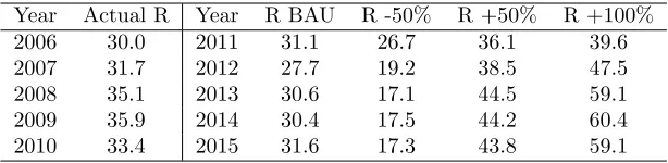
Table 4: Annual per acre f t3 harvest removals projections for private timberland in Maine using a 3 year moving
window. Values for 2006-2010 are from FIA data. Values for 2011-2015 are based on CEM matching and show the business as usual (BAU) projection along with stochastic increases in harvest levels of 50 and 100% and a reduction of 50%. Estimates are based on 3 year moving windows.
Year Actual R Year R BAU R -50% R +50% R +100%
2006 30.0 2011 31.1 26.7 36.1 39.6
2007 31.7 2012 27.7 19.2 38.5 47.5
2008 35.1 2013 30.6 17.1 44.5 59.1
2009 35.9 2014 30.4 17.5 44.2 60.4
2010 33.4 2015 31.6 17.3 43.8 59.1
for the scenarios (-50%,+50% and +100%) is not exactly attained. The removals (Tab. 4) are displayed for each scenario. They increase or decrease as expected depend-ing on the harvest scenarios, but reflect the stochastic nature of the process.
4.2 Application to Wisconsin data Wisconsin has enough national forest and state and local government land to make a comparison with privately owned land possible. The G/R values (Tab. 5) for national for-est land are quite variable. This is due to the rela-tively small number of FIA plots on national forest land in Wisconsin, and also because there is less harvesting on national forest land in general. Often, G/R ratios are shown as net-growth/removals. The values here are (gross growth)/(harvest removals), so mortality is not subtracted from growth.
Now we can look at the G/R projected trend for the 3 ownership types for years 2012-2016. The results (Tab. 6) suggest that the national forest could easily sustain a
doubling of harvest and still maintain a large G/R. The state and local government land could barely sustain a doubling of harvest, but it would border on being unsus-tainable. The private land could also sustain a harvest doubling, according to the G/R results, since the G/R values (Table 6) are all larger than 1.0 for the projected
Table 5: Gross-growth over harvest-removals ratios (G/R) for Wisconsin for National Forest (NF), state and local government (State), and private owners on timber-land computed with a 3 year moving window. Sample size is shown in parentheses.
Year NF State Private
years. Of course, other measures of sustainability should also be considered before such a drastic increase in har-vest levels is implemented.
Table 6: Projected gross-growth over harvest-removals ratios (G/R) for Wisconsin for National Forest (NF), state and local government (State), and private owners under scenarios that represent business as usual (BAU) harvesting and a doubling of harvest (+100%). These are 3 year moving windows applied to timberland.
NF State Private
Year BAU +100% BAU +100% BAU +100%
2012 5.067 3.365 2.437 1.739 2.960 2.210 2013 8.470 4.030 2.438 1.396 2.783 1.762 2014 9.036 4.437 2.427 1.039 1.643 1.390 2015 6.803 3.907 2.494 1.050 2.671 1.402 2016 5.462 3.450 2.634 1.055 2.755 1.462
5
Discussion
FIA data analysis has depended very heavily on the 5-year MA since the beginning of the annual inventory system around 1998. The MA has become linked to the concept of an EVALGRP, which is basically the most recent set of measurements for all FIA plots in a state. This linkage between an EVALGRP and the MA has be-come a standard analysis concept with FIA online tools, but it should be clear that the FIA sample design is not that restrictive. For example, the 3-year MW is a le-gitimate option, even though it does not align with any EVALGRP.
CEM was applied to FIA plots in the current EVAL-GRP, since those are the plots that are next in line to be remeasured. CEM identifies, for each subject plot in the current EVALGRP, already remeasured plots where the time 1 measurement matches the most recent measure-ment of the subject plot. Then the time 2 measuremeasure-ments from the matching plots can be used as predictions of what the subject plot will look like at its next measure-ment time.
CEM predictions combined with a 3-year or 5-year MW provide a simple way to estimate trends from FIA data that include the current year and a few projected years. Variance estimators that have been used for the 5-year MA can also be applied to the MW estimates. However, the same variance estimators applied to pro-jected years would understate the true uncertainty in the projections. It’s not clear that an unbiased estimator exists for the variance of projected means. One option would be to use methods developed for multiple imputa-tion (Rubin , 1987), which would involve applying CEM several times and combining the resulting variance esti-mates.
We did not compare CEM with other plot matching methods, such as those based on the propensity score or Mahalanobis distance. We deferred to the extensive work done elsewhere (Iacus et al. , 2011a,b) that demon-strates the improved performance of CEM over other methods. On the basis of that work, users can be confi-dent that the CEM process will result in good matches with respect to the coarsened variables that are selected by the user to describe the forest inventory plot data.
6
Conclusions
This study focused on FIA annual inventory plot data, but the methods should be applicable to any data base consisting of remeasured forest inventory plots. Methods were presented and demonstrated for estimating current trends and making short term projections. Few assump-tions are required to implement these methods. Annual estimates can be based on simple 3-year or 5-year mov-ing windows. Projections can be based on plot matchmov-ing techniques that eliminate the need for growth and yield models.
CEM was suggested as the plot matching method, be-cause it has desirable statistical properties and is easy to implement. In fact, CEM can be operationally im-plemented with standard SQL database programming. The focus here was on short term projections, which minimizes required assumptions and leads to a default BAU projection.
The short term projections were demonstrated with real data that was collected in the recent past. There-fore, the projections reflect what has occurred recently. This includes recent levels of disturbance, harvesting and land use change. Also, a method was developed to bias the projections to have increased frequency of an event type of interest. This provides an opportunity to imple-ment stochastic scenario developimple-ment. Scenarios involv-ing increasinvolv-ing levels of harvestinvolv-ing were demonstrated in the example applications.
It would be inadvisable to evaluate rare events or con-ditions with these methods, because few matches will be found in the database. Therefore, rare conditions would not be reliably projected. On the other hand, rare condi-tions are not likely to have reliable estimates for current values either, since there is typically only 1 FIA plot per 6000 acres. The methods here are recommended for short term projections, which should minimize the possi-bility that users would wrongly conclude that frequency of rare types is changing.
matches are found for a plot based on time 1 characteris-tics, then candidates that experience the event of interest are selected with a greater probability than candidates that don’t have the event. The event (harvesting in the examples) happens after time 1, so there is no determin-istic way to predict it. We think the stochastic biasing method is a good way to mimic reality in a model inde-pendent manner.
The example applications were implemented with a combination of SQL and R (R Development Core Team , 2010). These methods provide simple yet effective pro-cedures for extracting trend information from forest in-ventory data. The short term projections give a look ahead that requires few assumptions. Since the projec-tions are short term, they could be assessed for bias and perhaps improved by fine tuning the matching process every few years.
Acknowledgements
We thank the guest editors and the four anonymous reviewers for their helpful comments.
References
Bechtold, W. A., and P.L. Patterson. Editors. 2005. The enhanced forest inventory and analysis program -national sampling design and estimation procedures. Gen. Tech. Rep. SRS-80. Asheville, NC: U.S. Depart-ment of Agriculture, Forest Service, Southern Re-search Station. 85 p.
Dehejia, R.H., and S. Wahba. 2002. Propensity score-matching methods for nonexperimental causal studies. Rev. Econ. Stat. 84(1): 151-161.
Fernandez, C.A., and R. Astrup. 2012. Empirical har-vest models and their use in regional business-as-usual scenarios of timber supply and carbon stock develop-ment. Scand. J. For. Res. 27:379-392.
Iacus, S.M., G. King, and G. Porro. 2011a. Multivari-ate matching methods that are Monotonic Imbalance Bounding. J. Am. Stat. Assoc. 106(493): 345-361.
Iacus, S.M., G. King, and G. Porro. 2011b. Causal In-ference without Balance Checking: Coarsened Exact Matching. Polit. Anal. doi: 10.1093.
King, G., R. Nielsen, C. Coberley, J.E. Pope, and A. Wells. 2011. Comparative Effectiveness of Matching Methods for Causal Inference. Working Paper, 2011. Available online at http://j.mp/jCpWmk; last ac-cessed Feb. 25, 2013.
McRoberts, R.E. 2001. Imputation and model-based up-dating tech- niques for annual forest inventories. For. Sci. 47: 322-330.
R Development Core Team 2010. R: A language and environment for statistical computing. R Foundation for Statistical Computing, Vienna, Austria. ISBN 3-900051-07-0, Available online at http://www.R-project.org.
Reams, G.A., and J.M. McCollum. 2000. The use of multiple imputation in the southern annual forest in-ventory system. In Integrated Tools for Natural Re-source Inventories, Proceedings of IUFRO Conference. Edited by M.H. Hansen and T. Burk. USDA For. Serv. Gen. Tech. Rep. NC-212. pp. 228-233.
Reams, G.A. and P.C. Van Deusen. 1999. The South-ern Annual Forest Inventory System. J. Agric. Biol. Environ. Stat. 4(4): 346-360.
Roesch, F.A., J.R. Steinman, and M.T. Thompson. 2003. Annual forest inventory estimates based on the moving average. P. 21-30 in Proc. third annual forest inventory and analysis symp. October 17-19 2001, Traverse City, Michigan. McRoberts, R.E., G.A. Reams, P.C. Van Deusen, and J.W. Moser (eds.). Gen. Tech. Rep. NC-230, USDA For. Serv., North Central Res. Stn., St. Paul, MN. 208 p.
Rosenbaum, P.R., and D.B. Rubin. 1983. The central role of the propensity score in observational studies for causal effects. Biometrika 70(1): 41-55.
Rubin, D.B. 1987. Multiple imputation for nonresponse in surveys. John Wiley & Sons, Inc., New York, New York, USA. 258 p.
Rubin, D.B. 2001. Using Propensity Scores to Help Design Observational Studies: Application to the Tobacco Litigation. Health Serv. Outcomes Res. Methodol. 2:169-188.
Sande, I.G. 1983. Hot-deck imputation procedures. In: Madow WG, Olkin I, editors. Incomplete data in Sam-ple Surveys, vol. 3. New York: Academic Press: 334-50.
Van Deusen, P.C. 1997. Annual forest inventory statis-tical concepts with emphasis on multiple imputation. Can. J. For. Res. 27: 379-384.
Van Deusen, P.C. 1999. Modeling trends with annual survey data. Can. J. For. Res. 29: 1824-1828.
Wear, D.N. 2011. Forecasts of county-level land uses under three future scenarios: a technical document supporting the Forest Service 2010 RPA Assessment. Gen. Tech. Rep. SRS-141. Asheville, NC: U.S. Depart-ment of Agriculture Forest Service, Southern Research Station. 41 p.