Garcia

Forestry & Natural-Resource Sciences Last Correction: Apr. 4, 2018

REVERSE CAUSALITY IN SIZE-DEPENDENT GROWTH

Oscar Garc´ıa

Abstract.Size-dependent growth is likely to be growth-dependent size instead. Larger organisms do not

necessarily grow faster, but faster-growing ones always tend to be larger. This fact has been generally ignored. Correct causality structures are essential for plausible predictions outside the range of the data. Some techniques potentially useful for studying these issues are briefly described. In forestry, the relevance of multiple size measures like volume, height, diameter and basal area complicates the picture. Additionally, purely mathematical sources of growth-size correlations arise. Physiological considerations suggest avoiding stem thickness measures as explanatory variables in growth equations.

Keywords: Confounding, bias, consistency, path analysis, structural equation modelling, mixed

effects, endogenous variables, instrumental variables, allometry.

1

Introduction

Growth models typically utilize regressions of growth rate on size, possibly with additional independent vari-ables (Weiskittel et al. 2011). A causal relationship is usually implied, with growth rate depending on current size. Size-dependent growth is also the subject of theo-retical generalizations that have attracted much atten-tion (e.g. Damuth 2001, Sheil et al. 2017, and refer-ences therein). However, size is an accumulation of past growth, and therefore faster growth causes larger size, not necessarily the other way around. Although once stated this observation seems obvious, the only refer-ence related to biological growth that I have found is in Perry (1985): “past competitive interactions are in-tegrated in current tree size.” The statistical difficulties have been recognized in econometrics where, for a linear discrete-time growth model, least-squares estimation is known to be biased and inconsistent (Bun and Sarafidis 2015, this is discussed in detail below in Section 3).

Does it matter? The direction of causality may not be important for prediction in populations similar to the one originating the data. For instance, for yield forecast-ing of unmanaged or lightly managed forest stands, as in many growth model applications (Weiskittel et al. 2011). Or with intensive management where sufficient data is available, so that growing conditions are largely inter-polated rather than extrainter-polated (Goulding 1994). On the other hand, causality rather than just correlation is crucial for understanding process dynamics, and for

prediction under circumstances not represented in the data.

The section that follows explains further the statisti-cal confounding arising from causal ambiguity. Sections 3, 4 and 5 sketch some techniques that might help in understanding those issues, and perhaps eventually in dealing with them more effectively. All that assumes that “size” is expressed as a single number, typically biomass or volume. This is the case most commonly found in the literature, and demonstrates most clearly the main problems. Although a one-dimensional size can be appropriate for animals or annual plants, tree size is more accurately described by at least two dimen-sions, height and radius (or diameter, circumference or cross-sectional area). Longitudinal and radial growth derive from different meristems, and respond differently to various growing conditions. This multivariate descrip-tion complicates things, giving rise to addidescrip-tional, purely mathematical, sources of correlation that are discussed in Section 6. The paper closes with a Conclusions sec-tion.

2

The problem

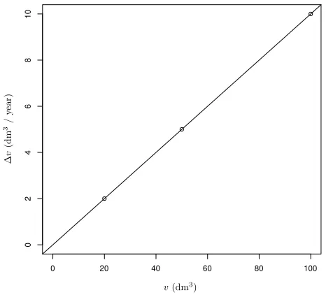
A minimal example may be useful for exposing the es-sentials (Lee and Garc´ıa 2016). Assume that tree annual volume increment ∆v in a forest stand is constant over time, and that it is not affected by tree size. Neverthe-less, ∆v varies among trees due to genetics, microsite, competition, or other factors. Take 3 trees with incre-ments of 2, 5, and 10 dm3/ year. The tree volumesvat

age 10 are 10 times the increment, i.e., 20, 50, and 100 dm3. Plotting increment over size (Figure 1) indicates a perfect regression model ∆v= 0.1v (or more generally, ∆v =v/t). This model produces exact predictions for trees of any size, but it is biologically “wrong”, in the sense that in this instance ∆v does not causally depend onv. The example could be embellished by introducing growth variability and measurement error, and by using larger samples of trees. Then the regression would not be error-free, but the predictions would still be better than those from any model not includingv as a predic-tor. The wrong model is best.

Figure 1: Artificial example of a perfect non-causal relation-ship, estimating tree volume growth increment from current tree volume (see text).

Lee and Garc´ıa (2016) analyzed real growth data from spruce-hardwoods mixtures in British Columbia. The best tree volume growth rate estimates not using cur-rent volume had R2values of 0.62 with spatially explicit competition indices, and 0.75 with distance independent competition indices1. In contrast, a simple linear regres-sion ∆v=β0+β1vhad R2 = 0.86.

In general, consider a regression for growth rate

∆y=f(y,x), (1)

where y = y(t) is current size, and x is a vector of additional independent variables. The dependent

vari-1_{Unlike most competitions indices, those used in the study did}

not contain embedded tree diameter measurements. Presumably the perfect plasticity assumption behind the aspatial indices is better than the assumption of no plasticity in the spatial ones (Strigul et al. 2008).

able ∆y could be an annual incrementy(t+ 1)−y(t), a periodic increment y(t +k)− y(t) or [y(t + k)−

y(t)]/k, or even an instantaneous increment in continu-ous time, dy/dt. In forestry, these regressions have been called self-referencing models (Northway 1985, Strub and Cieszewski 2012). Because y is an accumulation of past values of ∆y for each individual, in a heteroge-neous population the two variables are correlated. That can produce good fit statistics, even if ∆yis not causally dependent on y. The fit is good not necessarily be-cause larger individuals grow faster, but bebe-cause faster-growing individuals tend to be larger. Predictions are based essentially on an extrapolation of past growth rates (Lee and Garc´ıa 2016). The extrapolation can fail if there is a change in the growing conditions that pre-vailed in the sample (e.g., Russell et al. 2015).

Of course, students of statistics are taught that corre-lation is not causation, and that models should not be used outside the range of the data. But the first point is often forgotten in the interpretation of research results. And models are invariably pushed beyond the comfort zone. After all, if we had enough data for all the condi-tions of interest there would be little need for models.

3

The dynamic panel data model in

econometrics

Panel data consists of observations at consecutive times t = 1,2, . . . , T on each of N items or individu-als i = 1,2, . . . , N. The (linear) dynamic panel data model can be written as

yit=αyi,t−1+β0xit0 +u_it. (2)

Here the vector xit0 may include various regressors

ob-served at times such ast0 =t,t0 =t−1,t0 =t−2, etc. The error termuitvaries across individuals as

uit=λi+it, (3)

whereλi isunobserved individual heterogeneity, and the

it are errors with mean 0 and equal variance,

indepen-dent across individuals and times.

The yit depend on the value of λi, so that in

par-ticular the regressor yi,t−1 and the error uit in eq. (2)

are correlated. In econometric terminologyyi,t−1 is

en-dogenous (correlated with the error term), as opossed toexogenous(independent of the error term as assumed in standard linear regression). Consequently, it is found that the ordinary least-squares (OLS) estimate of α is biased. Worse, OLS is inconsistent, that is, estimates do not converge to the true values asN → ∞for fixedT.

as

yi,t+1=αyit+β0xit+uit, (4)

making use of the fact thatuithas the same distribution

for allt. Then,

∆yit=yi,t+1−yit= (α−1)yit+β0xit+λi+it. (5)

Bun and Sarafidis (2015) review estimation meth-ods for the dynamic panel data model, and point out that there is an implicit stationarity assumption. That might not be suitable for biological growth modelling, where interest focuses on transients far from a steady state. Econometric methods may or may not be useful for growth parameter estimation, but the main point is the recognition that OLS fails when size appears on the right-hand side of the growth rate regression.

4

A mixed effects view

A key property of the dynamic panel data model is the presence of individual heterogeneity,λi. More generally,

the regression model of eq. (1) may be written as

∆yit=f(yit,xit,γ,λi, it), (6)

for observations on individuals i = 1, . . . , N at times

t = ti1, . . . , ti,Ti. In growth data the number and

tim-ing of measurements on each individual and the time intervals can vary. The local parameters λi are specific

to individuali, while theglobal parameters γ are com-mon to all. In econometrics, locals are called incidental parameters, globals are called structural, and it is an

idisioncratic error.

For instance, the minimal example of Section 2 might be written as

∆vit=γvit+λi+it, (7)

where we assumedγ= 0,λ1= 2,λ2= 5, and λ3 = 10,

andit was ignored.

The model of eq. (6) could be estimated, for in-stance, by maximum likelihood. The locals can be con-sidered either as fixed unknown individual-specific pa-rameters, or as random variables representing sampling from some hypothetical meta-population of individuals (Garc´ıa 2017b, Sec. 3.3). The random locals alternative is far more popular nowadays, corresponding to a mixed effects model. The parameters could be estimated with mixed-effects software. Note however that, as indicated in Section 2, standard fit statistics will be worse than those for the “wrong” model that ignores individual het-erogeneity.

5

Path analysis and structural

equa-tion models

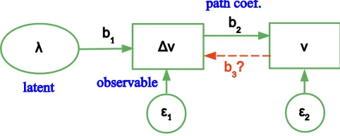
Path analysis is a technique for studying causal re-lationships, developed by Sewell Wright in the 1920’s

(Wright 1921, Bollen 2005a). Later, inference methods were refined in Structural Equation Modelling (SEM; Bollen 2005b, Fox 2006, Umbach et al. 2017). Applica-tions have been mostly in the social sciences, but more recently biological uses have increased (Iriondo et al. 2003, Lamb et al. 2011).

The approach allows for testing postulated causal models, assessing if they are consistent with the data. The model is commonly visualized in a path diagram. Figure 2 shows a tentative path diagram for the exam-ple of Section 2. Variables are classified as observed, unobserved (also calledlatent), or disturbances (errors). Each observed variable is enclosed in a box. Latent vari-ables appear in ellipses or ovals. Errors are not enclosed in either, or are sometimes placed in ovals or circles since they are also unobserved. Arrows between variables in-dicate direct causal influences (paths). In path analysis, apath coefficient associated to each path is calculated.

Δv v

λ

ε ε

b₁ b2

path coef.

observable latent

b

3?

1 2

Figure 2: A path diagram for the model behind the example of Section 2. The dashed arrow represents a possible “real” size effect.

For the example,vand ∆vare the observed variables size and growth rate, respectively. The unobserved vari-ableλrepresents the growth rate intrinsic to each tree. Together with random variation (assumed to be 0 in the numerical example), it determines the actual growth in-crement. Growth increments cause the size to increase. A size observation error has been included in the dia-gram. SEM could be used to evaluate the consistency of this model with observed data, and to compare it to an alternative that adds a direct causal effect of size on growth, represented by the dashed arrow (γ 6= 0 in eq. (7)).

6

Which size?

depending on past stand densities. Therefore, allometric relationships that estimate volume or biomass from di-ameter can only be accurate for growing conditions sim-ilar to those in the data from which they are derived2_.

It follows that uni-dimensional growth-size relation-ships are unsatisfactory for trees and forests. It is nec-essary to take into account simultaneously the dimen-sional components: at least height, diameter, and in for-est stands, number of trees.

Confusion also arises from the use of different variables in growth-size relationships: biomass or volume, or the more easily obtained diameter or basal area. In fact, the behavior of their increments is quite different, as shown by Assmann (1970, p. 151). His result for stand volumevs basal area can be easily proved in continuous time, with instantaneous increments denoted as ˙V = dV /dt. Assume that V =α+βBH, where V is stand volume,B is basal area per hectare, and H is mean or top height (for simplicity we avoid the volume as product of basal area and form-height used by Assmann). Then, differentiating,

˙

V =β( ˙BH+BH˙). (8)

This is essentially equivalent to Assmann’s equation. Solving for ˙B gives

˙

B =

˙

V

βH −

˙

H

HB , (9)

which shows that even if ˙V is independent of size, ˙Bdoes depend onB (andH). Similarly, Lee and Garc´ıa (2016) show that if a tree volume is approximated in terms of tree dbhdand heighthbyα+βd2h,

˙

d= v˙ 2βhd−

˙

hd

2h . (10)

For models to have a chance of performing acceptably outside the range of the data, they need to reflect the causal logic of the biological processes. Good fit statis-tics for purely empirical relationships are not sufficient. It makes sense to have growth in biomass, or in its proxy stem volume, as a dependent variable reflecting carbon capture and accumulation. Height influences the costs of evapotranspiration, and also dominance relationships in the case of individual trees or cohorts, so that it is a reasonable predictor. Stand density is also an important factor. Stem diameter, however, reflects the accumula-tion of mostly dead xylem on the stems, and there is little physiological justification for including it on the equation right-hand sides; the same is true for volume or basal area (Garc´ıa 2017a).

2_{Allometry is used here in the original sense of Huxley (1932),}

a (usually power) function of a single independent variable. The term is often misused as referring to any arbitrary volume or biomass function.

7

Conclusions

Size-dependent growth may actually be growth-dependent size. The direction of causality is not impor-tant for management that does not deviate markedly from the conditions represented in the data. Empiri-cal extrapolation of past growth can be highly effective. Increasingly though, models are applied to new situ-ations, including natural or management disturbances and environmental change. Understanding the system and proper causal modelling are then essential.

It can be difficult to disentangle the true causal ef-fects, although mixed-effects modelling, path analysis and structural equation models seem promising tools. My presentation of those topics has been brief and ten-tative. I admit not fully understanding all aspects of the problem and of the techniques, and that some of the details might not be entirely correct. Obviously, more research is needed. But I believe that the important point is to get researchers to recognize that there is a problem, something that has not happened.

With trees and forests, simple one-dimensional growth-size models are unsatisfactory, because size com-ponents like height and diameter are important and re-act differently to growing conditions. Purely mathemati-cal sources of correlation from these variables complicate the picture. Multidimensional systems of growth equa-tions are needed. Still, adequate causal structures are essential if forecasts for previously unobserved situations are desired. In particular, it is suggested that diameter and basal area should be banished from the right-hand side of growth equations (Garc´ıa 2017a). Experiments might be useful where tree size and growing conditions are uncoupled, e.g., through randomized (not selective) thinning.

Acknowledgements

I am grateful to anonymous reviewers for suggestions that contributed to improve the text.

References

Assmann, E., 1970. The Principles of Forest Yield Study. Pergamon Press, Oxford, England. 506 p.

Bollen, K. A., 2005a. Path analysis. In Encyclopedia of Biostatistics, volume 6, Armitage, P., and T. Colton, eds., second edition, pp. 3973–3977. Wiley.

Bollen, K. A., 2005b. Structural equation models. In Encyclopedia of Biostatistics, volume 6, Armitage, P., and T. Colton, eds., second edition, pp. 5269–5278. Wiley.

Baltagi, B. H., ed., chapter 3, pp. 76–110. Oxford Uni-versity Press.

Damuth, J., 2001. Scaling of growth: Plants and ani-mals are not so different. Proceedings of the National Academy of Sciences 98(5):2113–2114.

Fox, J., 2006. Teacher’s corner: Structural equation modeling with the sem package in R. Structural Equa-tion Modeling 13(3):465–486.

Garc´ıa, O., 2017a. Cohort aggregation modelling for complex forest stands: Spruce-aspen mixtures in British Columbia. Ecological Modelling 343:109–122.

Garc´ıa, O., 2017b. Estimating reducible stochas-tic differential equations by conversion to a least-squares problem. ArXiv e-prints (arXiv:1710.06021 [stat.ME]). URL: https://arxiv.org/abs/1710.06021.

Goulding, C. J., 1994. Development of growth models forPinus radiata in New Zealand — experience with management and process models. Forest Ecology and Management 69(1–3):331–343.

Huxley, J. S., 1932. Problems of Relative Growth. Methuen & Co., London. (Second Edition, Dover 1972).

Iriondo, J. M., M. J. Albert, and A. Escudero, 2003. Structural equation modelling: an alternative for as-sessing causal relationships in threatened plant popu-lations. Biological Conservation 113(3):367–377.

Lamb, E., S. Shirtliffe, and W. May, 2011. Structural equation modeling in the plant sciences: An example using yield components in oat. Canadian Journal of Plant Science 91(4):603–619.

Lee, M. J., and O. Garc´ıa, 2016. Plasticity and extrap-olation in modeling mixed-species stands. Forest Sci-ence 62(1):1–8.

Northway, S. M., 1985. Notes: Fitting site index equa-tions and other self-referencing funcequa-tions. Forest Sci-ence 31:233–235.

Perry, D. A., 1985. The competition process in forest stands. In Attributes of Trees as Crop Plants, Cannell, M. G. R., and J. E. Jackson, eds., chapter 28, pp. 481– 506. Institute of Terrestrial Ecology, Abbots Ripton, Hunts, England.

Russell, M. B., A. W. D’Amato, M. A. Albers, C. W. Woodall, K. J. Puettmann, M. R. Saunders, and C. L. VanderSchaaf, 2015. Performance of the Forest Vege-tation Simulator in managed white spruce planVege-tations influenced by Eastern spruce budworm in Northern Minnesota. Forest Science 61(4):723–730.

Sheil, D., C. S. Eastaugh, M. Vlam, P. A. Zuidema, P. Groenendijk, P. van der Sleen, A. Jay, and J. Van-clay, 2017. Does biomass growth increase in the largest trees? Flaws, fallacies and alternative analyses. Func-tional Ecology 31(3):568–581.

Strigul, N., D. Pristinski, D. Purves, J. Dushoff, and S. Pacala, 2008. Scaling from trees to forests: Tractable macroscopic equations for forest dynamics. Ecological Monographs 78(4):523–545.

Strub, M., and C. Cieszewski, 2012. The compara-tive R2 and its application to self-referencing mod-els. Mathematical and Computational Forestry & Natural-Resource Sciences (MCFNS) 4(2):73–76.

Umbach, N., K. Naumann, H. Brandt, and A. Kelava, 2017. Fitting nonlinear structural equation models in R with package nlsem. Journal of Statistical Software 77(7):1–20.

Weiskittel, A. R., D. W. Hann, J. John A. Kershaw, and J. K. Vanclay, 2011. Forest Growth and Yield Modeling. Wiley-Blackwell. 430 p.