Potential-Function Proofs for Gradient Methods

www.theoryofcomputing.org

RESEARCH SURVEY

Potential-Function Proofs

for Gradient Methods

Nikhil Bansal

Anupam Gupta

Received March 3, 2019; Revised August 6, 2019; Published September 12, 2019

Abstract: This note discusses proofs of convergence for gradient methods (also called “first-order methods”) based on simple potential-function arguments. We cover methods like gradient descent (for both smooth and non-smooth settings), mirror descent, and some accelerated variants. We hope the structure and presentation of these amortized-analysis proofs will be useful as a guiding principle in learning and using these proofs.

1

Introduction

The “gradient descent” framework is a class of iterative methods for solving convex minimization problems—indeed, since the gradient gives the direction of steepest increase in function value, a natural approach to minimize the convex function is to move in the direction opposite to the gradient. Variants of this general versatile approach have been central to convex optimization for many years. In recent years, with the increased use of continuous methods in discrete optimization, this technique has also become central for algorithm design in general.

∗_{Supported in part by NWO Vici grant 639.023.812 and an ERC consolidator grant 617951.}

†_{Supported in part by NSF awards CCF-1536002, CCF-1540541, and CCF-1617790.}

ACM Classification:G.1.6

AMS Classification:68Q25

In this note we give convergence arguments for many commonly studied versions of gradient methods (also referred to as “first-order methods”) using simple potential-functionarguments. We find that presenting the proofs in the amortized-analysis framework is useful as a guiding principle, since it imparts a clear structure and direction to proofs. We hope others will also find this perspective useful, both in learning and teaching these techniques and proofs, and also in extending them to other domains.

A disclaimer: previously existing proofs for gradient methods are usually not difficult, and their individual components are not substantially different from the ones in this note. However, using an explicit potential to guide our proofs makes them arguably more intuitive. In fact, the intuition of viewing these gradient methods as trying to control a potential function is also known to the specialists; e. g., see the text of Nemirovski and Yudin [18, pp. 85–88] for a continuous perspective via Lyapunov functions. This is more explicit in recent papers [24,29,17,30, 8] relating continuous and discrete updates to understand the acceleration phenomenon, e. g., Krichene et al. [17] give the potential function we use in §5.2. However, these potential-function proofs and intuitions have not yet permeated into the commonly presented expositions. The current note is an attempt to make such ideas more widely known.

Basic definitions. Recall that a set K ⊆Rd is convex if for all x,y∈K, the convex combination λx+ (1−λ)y∈Kfor allλ ∈[0,1]. A function f :Rd→Risconvexover a convex setKif

f(λx+ (1−λ)y)≤λ f(x) + (1−λ)f(y) ∀x,y∈K,∀λ ∈[0,1].

This is called thezeroth-orderdefinition. There are other equivalent notions: if the function is differen-tiable, thefirst-orderdefinition is that f is convex overKif

f(y)≥ f(x) +h∇f(x),y−xi ∀x,y∈K. (1.1) (Thesecond-order definition says that a twice-differentiable f is convex if its Hessian matrix∇2f is positive-semidefinite.) For this note, we assume our convex setsKare closed, and the convex functions f are differentiable. However, the proofs extend to non-differentiable functions in the natural way, using subgradients. (See, e. g., [13] for more definitions and background on convexity and subgradients.)

The problems. Given a convex function f :Rd→R, and an error parameterε, the(unconstrained) convex minimizationproblem is to find a pointx_bsuch that f(_bx)−minx∈_Rd f(x)≤ε. In theconstrained version of the problem, we are also given a convex setK, and the goal is to find a pointxb∈Kwhich has

error f(bx)−minx∈K f(x)≤ε. In either case, letx

∗_{denote the minimizer for f(·). We will be interested} in bounding the number of gradient queries required to converge to the approximate minimizerx, as a_b function of the distance betweenx0 andx∗and some parameters of the function f, depending on the

particular variant of gradient descent.

Assumptions. We assume that our convex functions are closed, convex, and differentiable, and that the convex setsKare also closed with non-empty interior. We assume access to a gradient oracle for each of the functions ft we consider, i. e., given any pointx, we can get the gradient∇ft(x)of function ft at pointx. We only work with the Euclidean normk·k₂for the first few sections; general norms are discussed from §4onwards.

References. In this survey, we focus only on the exposition of the proofs. We omit most citations, and also discussion of the “bigger picture.” There are many excellent sources for other proofs of these results, with comprehensive bibliographies; e. g., see the classic text by Shor [23], the authoritative notes by Nesterov [20], and Ben-Tal and Nemirovski [3], the monographs of Bubeck [6] and Shalev-Shwartz [22], the textbooks by Cesa-Bianchi and Lugosi [7], Hazan [12], and lecture notes by Duchi [10] and Vishnoi [28].

There are several other perspectives on these proofs that the reader may find useful. One useful perspective is that of viewing these methods as discretizations of suitable continuous dynamics; this appears even in the classic work of Nemirovski and Yudin [18], and has been widely used recently (see, e. g., [24,29,17,30]). Another useful perspective is exhibit a “dual” lower bound on the optimal value via the convex conjugate, and use the duality gap to bound the error (see, e. g., [8,21]). We refer the interested reader to the respective papers for more details.

Finally, we discuss some concurrent and related work. Independently of our work, Karimi and Vavasis [15] give potential-based convergence proofs for conjugate gradient and accelerated methods; their potentials are similar to ours. And following up on a preprint of our results, Taylor and Bach [26] analyze stochastic gradient methods using potential functions.

1.1 Results and organization

All of the proofs use the same general potential: for some fixed pointx∗(which can be thought of as the optimal or reference point) we have

Φt =at·(f(xt)−f(x∗)) +bt·(distance fromxt tox∗). (1.2) Hereat,btare non-negative, and naturally, different proofs use slightly different choice of these multipliers, and even the distance functions may vary. However, the general approach remains the same: we show thatΦt+1−Φt≤Bt (whereBt is often zero). Since the potential and distance terms remain non-negative, the telescoping sum gives

ΦT ≤Φ0+

T−1

∑

Bt =⇒ f(xT)−f(x∗)≤

Φ0+∑tBt aT

.

(plusB). I. e., ft(xt) + (Φt+1−Φt)≤ ft(x∗) +B. This telescopes to imply that the average regret is 1

T T

∑

(ft(xt)−ft(x∗))

!

≤B+Φ0

T .

The potential here is very simple: we setat =0 and just use the distance of the current pointxt to the optimal pointx∗(according to the “right” distance). For example, for basic gradient descent, the potential is just a scaled version ofkxt−x∗k2.

Next, we give proofs of convergence for the case ofsmoothconvex functions in §3. In the simplest case we just setbt=0 and useat=tin (1.2) to proveBt≈1/t. This gives an error of≈(logT)/T, which is in the right ballpark. (This can be optimized using better settings of the multipliers.) The proofs for projected smooth gradient descent, gradient descent for well-conditioned functions, and the Frank–Wolfe method, all follow this template. For these proofs, we now use the “value-based” terms in (1.2), i. e., the terms that depend on f(xt)−f(x∗).

We then extend our understanding tomirror descent. This is a substantial generalization of gradient descent to general norms. While the language necessarily becomes more technical (relying on dual norms and Bregman divergences), the ideas remain clean. Indeed, the structure of the potential-based proofs from §2remains essentially the same as for basic gradient descent; the potential is now based on a Bregman divergence, a natural generalization of the squared distance. These proofs appear in §4.

An orthogonal extension is to potential-based proofs of Nesterov’s accelerated gradient descent method for smooth and well-conditioned convex functions. The ideas in this section build on the simple calculations we would have seen in §2and §3. We can now use the full power of both distance-based and value-based terms in the potential function (1.2), trading them off against each other. Moreover, in §5.1 we show how the basic analysis for smooth convex functions from §3directly suggests how to obtain the accelerated algorithm by coupling together one cautious and one aggressive gradient descent step.

Organization. The paper follows the above outline. We start with proofs for general convex functions in §2 using simple distance-based potentials, then proceed to smooth and well-conditioned convex functions in §3using more sophisticated potentials. We then discuss the generalization to mirror descent via Bregman divergences in §4. Finally, we give proofs for accelerated versions in §5. Note that §4and §5are independent, and may be read in either order.

2

Online analyses

2.1 Basic gradient descent

The basic analysis works even for the online convex optimization case: at each step we are given a function ft, we playxt, and want to minimize the regret. In this case the update rule is:

xt+1←xt−ηt∇ft(xt) . (2.1) An equivalent form for this update, that is easily verified by taking derivatives with respect tox, is:

xt+1←arg min

x

n1

2kx−xtk

2₊

ηthx,∇ft(xt)i

o

Intuitively, we want to move in the direction of the negative gradient, but do not want to move too far.

Theorem 2.1(Basic gradient descent). Let f₁, . . . ,fT :Rn→Rbe G-Lipschitz functions, i. e.k∇ft(x)k ≤ G for all x,t. Then starting at point x0∈Rnand using updates (2.1) with step size

ηt=η= D G√T for T steps guarantees an average regret of

1 T

T−1

∑

ft(xt)−ft(x∗)

≤ηG

2

2 + D2 2ηT ≤

DG √

T , for all x∗withkx0−x∗k ≤D.

Proof. Consider the potential function

Φt = 1

2ηkxt−x ∗_k2

(2.3)

which is positive for allt. We show that, for some upper boundB,

ft(xt)−ft(x∗) +Φt+1−Φt ≤B. (2.4) Summing over all timest, the average regret is

1 T

T−1

∑

(ft(xt)−ft(x∗))≤B+ 1

T(Φ0−ΦT)≤B+

Φ0

T =B+ D2

2ηT. (2.5)

Now we can computeB, and then balance the two terms. While the potential uses differences of the formxt−x∗, the key is to express as much as possible in terms ofxt+1−xt, because the update rule (2.1) implies

xt+1−xt=−η∇ft(xt). (2.6)

The change in potential. Using thatka+bk2− kak2=2ha,bi+kbk2for the Euclidean norm, 1

2(kxt+1−x

∗_k2_{− kx}

t−x∗k2) =hxt+1−xt,xt−x∗i+ 1

2kxt+1−xtk

2

=ηth∇ft(xt),x∗−xti+ ηt2

2 k∇ft(xt)k

2

. (2.7)

The amortized cost. Settingηt=η for all steps, ft(xt)−ft(x∗) +Φt+1−Φt

=ft(xt)−ft(x∗) +h∇ft(xt),x∗−xti+ η

2k∇ft(xt)k

2

(by (2.7))

≤0+η

2k∇ft(xt)k

2 _≤ ηG2

2 (by convexity, and the bound on gradients.) Substituting forBin (2.5) and simplifying withη=D/(G

√

K

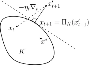
x

−

η

∇

x

x

= Π

(

x

)

x

Figure 1: Projected Gradient Descent.

The regret bound implies a convergence result for the offline case, i. e., for the case where ft = f for allt. Here, setting_bx:= (1/T)∑tT=−01xt shows

f(xb)−f(x

∗

) = f

1 T

∑

−f(x∗)≤ 1

T

∑

))≤√DG T ≤ε, as long asT ≥(DG/ε)2andη=ε/G2.

If the time horizonT is unknown, setting a time-dependent step size ofηt =D/(G √

t)works, with an identical proof. It is also well-known that the convergence bound above is the best possible in general, modulo constant factors (see, e. g., [20, Thm 3.2.1] or [6, Thm 3.13]).

2.1.1 Projected gradient descent

If we want to solve the constrained minimization problem for a convex bodyK, we update as follows:

x0_t+1←xt−η∇ft(xt), xt+1←ΠK(xt0+1).

(2.8) (2.9)

whereΠK(x0):=arg minx∈Kkx−x0kis the projection ofx0onto the convex bodyK. SeeFigure 1.

Proposition 2.2(Pythagorean property). Given a convex body K⊆_Rn_{, let a∈K and b}0_∈

Rn. Let b=ΠK(b0). Thenha−b,b0−bi ≤0. Henceka−bk2≤ ka−b0k2.

Proof. For the first part, the separating hyperplane atbhasb0 on one side, and all ofK(and hencea) on the other side. Hence the angle betweenb0−banda−bmust be obtuse, giving the negative inner product. For the second part,ka−b0k2=ka−bk2+kb−b0k2+2ha−b,b−b0i. But the latter two terms are positive, which proves the lemma.

Using this, we get that for any pointx∗∈K,

kxt+1−x∗k2≤ kx0t+1−x

Using the same potential function (2.3), this inequality implies: ft(xt)−ft(x∗) +Φt+1−Φt≤ ft(xt)−ft(x∗) +

1 2η(kx

0

t+1−x∗k2− kxt−x∗k2),

or in other words, the projection only helps and we can follow the analysis from §2.1starting at (2.7) to bound the amortized cost byηG2/2. So this gives a regret bound identical to that ofTheorem 2.1.

2.2 Strong convexity analysis

Let us a prove a better regret (and convergence) bound when the functions are “not too flat.” A function f over a convex setKisα-strongly convex, whereα≥0, if for allu,v∈K

f(λu+ (1−λ)v)≤λf(u) + (1−λ)f(v)−α

2λ(1−λ)kv−uk

2 _(2.10)

for allλ ∈[0,1]. For the case of differentiable functions, this is equivalent to saying that for allx,y∈K, f(y)≥ f(x) +h∇f(x),y−xi+α

2ky−xk

2_{. (2.11)}

Forα-strongly convex functions ft, we use the same update step but vary the step sizeηt. Specifically, xt+1←ΠK(xt−ηt∇ft(xt)) , (2.12) whereηt=1/(α(t+1)).

Theorem 2.3(Strongly convex functions). If the functions ft areα-strongly convex and G is an upper bound onk∇ft(x)kfor all x∈K, the update rule (2.12) withηt=1/(α(t+1))guarantees an average regret of

1 T

T−1

∑

ft(xt)−ft(x∗)

≤G

2_logT

2Tα . Proof. The potential function is now

Φt = 1 2ηt−1

kxt−x∗k2= tα

2 kxt−x

∗_k2 _{. (2.13)}

The change in potential. Letx_t0₊₁:=xt−ηt∇ft(xt)denote the intermediate point after the gradient step, but before performing the projection.

Φt+1−Φt =

α(t+1)

2 kxt+1−x

∗_k2₋αt

2 kxt−x ∗_k2

=α

2kxt−x

∗_k2₊ 1

2ηt

kxt+1−x∗k2− kxt−x∗k2

≤α 2kxt−x

∗_k2

+ 1

2ηt

kx0_t+1−x∗k2− kxt−x∗k2

(by Prop.2.2)

=α

2kxt−x ∗_k2

+h∇ft(xt),x∗−xti+ ηt

2k∇ft(xt)k

2

The amortized cost.

ft(xt)−ft(x∗) +Φt+1−Φt ≤ ft(xt)−ft(x∗) +

α 2kxt−x

∗_k2_+h

∇ft(xt),x∗−xti

| {z }

≤0 byα-strong convexity

+ηt

2k∇ft(xt)k

2

≤ ηt

2k∇ft(xt)k

2 _≤ ηtG2

2 (by bound on gradients). (2.14)

Now summing over all time stepst, the total regret is

∑

(ft(xt)−ft(x∗))≤Φ0+

_∑

t ηt

2G

2_≤0+G2logT

2α .

Hence total regret only increases logarithmically as logT with time if the ft are strongly convex, as opposed to√T inTheorem 2.1.

This bound ofO(logT)on the average regret is tight: Takimoto and Warmuth [25] show a matching lower bound. However, in theofflineoptimization setting where we have a fixed function ft =f, using the same analysis but a better averaging shows a convergence rate ofO(1/T)with respect to a convex combination of the pointsxt.

Theorem 2.4(Strongly convex functions: Take II). Let f beα-strongly convex with gradients satisfying k∇f(x)k ≤G for all x, and xtbe the iterates produced by applying the update rule (2.1) withηt=1/(αt). For any T≥1, let xT :=∑tT=1λtxt denote the convex combination of xt with

λt= 2t T(T+1).

Then,

f(xT)−f(x∗)≤ G2 α(T+1).

Proof. Instead of summing up (2.14) directly overtin the regret analysis above, we first multiply (2.14) byt, and then sum overtto obtain

T

∑

t(ft(xt)−ft(x∗))≤ 1 2αT G

2_.

Using ft= f and dividing byT(T+1)/2 throughout, and by the convexity of f we obtain

f(xT)−f(x∗)≤ G2 α(T+1).

3

Bounds for smooth functions

We now turn to the setting where the functions are Lipschitz smooth, i. e., when the gradient does not change too rapidly. We know that in the online case, the average regret ofO(1/√T)is tight even for linear functions [7]. However we get better guarantees for theofflinesetting where the function ft =f for all time steps. The potential functions now look more like (1.2), and use the difference(f(xt)−f(x∗))in function value, not just in action space.

Define a function f to beβ-Lipschitz smooth(or simplyβ-smooth) if for allu,v

f(λu+ (1−λ)v)≥λf(u) + (1−λ)f(v)−β

2λ(1−λ)kv−uk

2 _(3.1)

for allλ ∈[0,1]. For the case of differentiable functions, this is equivalent to saying that forx,y, we have

f(y)≤ f(x) +h∇f(x),y−xi+β

2ky−xk

2_{. (3.2)}

Observe the inequalities here are in the opposite directions from the definitions of convexity (1.1) and strong-convexity (2.11). Indeed, smoothness implies that the function does not “grow too fast” anywhere. The smoothness condition is equivalent to requiring that the gradients are Lipschitz continuous, i. e., k∇f(x)−∇f(y)k2≤βkx−yk2for allx,y.

3.1 Smooth gradient descent

The update rule in this case has a time-invariant multiplier (where we use∇t :=∇f(xt)for brevity).

xt+1←xt− 1

β ∇t . (3.3)

We first show an analysis based on a very natural potential, that gives a slightly sub-optimal bound with an additional logT factor. We improve this later by slightly modifying the potential.

Theorem 3.1(Smooth functions). If f isβ-smooth and D:=maxx{kx−x∗k₂| f(x)≤f(x0)}, the update

rule (3.3) guarantees

f(xT)−f(x∗)≤β D

2_(1+lnT)

2T .

Proof. To show a convergence rate of O(1/t), perhaps the most natural approach is to consider the potential

Φt =t·(f(xt)−f(x∗))

The potential change.

Φt+1−Φt= (t+1)(f(xt+1)−f(x∗))−t(f(xt)−f(x∗))

= (t+1)(f(xt+1)−f(xt)) + (f(xt)−f(x∗)). (3.4) To bound the first term, we use the smoothness of f withx=xt andy=xt+1=xt−ηt∇t:

f(xt+1)≤ f(xt)−ηt· k∇tk₂2+β₂·ηt2· k∇tk2₂. The choice ofηt=1/β minimizes the right hand side above to give

f(xt+1)≤ f(xt)−₂1_βk∇tk2₂. (3.5) For the second term in (3.4), just use convexity and Cauchy-Schwarz:

f(xt)−f(x∗)≤ h∇t,xt−x∗i ≤ k∇tk2· kxt−x∗k2 (3.6)

≤1_/2(ak∇tk2+ (1/a)kxt−x∗k2),

for any parametera>0. Note that (3.5) ensures that f(xt)≤ f(xt−1)≤ · · · ≤ f(x0), so let us define

D:=max{kx−x∗k₂|f(x)≤ f(x0)}. So the potential change is

Φt+1−Φt ≤(t+1)·(−₂1_β)k∇tk2₂+1₂ (ak∇tk2₂+D2/a). (3.7) Choosinga= (t+1)/βcancels the gradient terms. Hence the potential increase is at mostD2β/(2(t+1)), and

f(xT)−f(x∗) =

ΦT T =

1 T

T−1

∑

(Φt+1−Φt)≤ 1 T

T−1

∑

D2

2(t+1)β ≤β

D2(1+lnT)

2T .

The intuition is evident from (3.5) and (3.6): we improve a lot by (3.5) when the gradients are large, or else we are close to the optimum by (3.6).

A tighter analysis. The logarithmic dependence inTheorem 3.1can be removed by a simple trick of multiplying the potential by a linear term int, which avoids the sum over 1/t.

Theorem 3.2(Smooth functions: Take II). If f isβ-smooth, and D:=maxx{kx−x∗k₂| f(x)≤f(x0)},

the update rule (3.3) guarantees

f(xT)−f(x∗)≤β 2D2 T+1. Proof. Consider the following potential

Φt=t(t+1)·(f(xt)−f(x∗)) . The potential change is

Plugging in (3.5) and (3.6) gives

≤(t+1)(t+2)·−1 2βk∇tk

2_{+2(t+1)· k}

∇tk2·D≤2D2β·t+1 t+2,

where the last inequality is the maximum value of the preceding expression obtained at k∇tk = 2βD/(t+2). Summing over the time steps,ΦT ≤T·2D2β, so

f(xT)−f(x∗)≤

2D2β·T T(T+1) =β

2D2 T+1.

3.1.1 Yet another proof

Let’s see yet another proof that gets rid of the logarithmic term. Interestingly, the potential function now combines both the difference in the function value, and the distance in the “action” space.

Theorem 3.3(Smooth functions: Take III). If f isβ-smooth, the update rule (3.3) guarantees f(xT)−f(x∗)≤β

kx₀−x∗k2 2T . Proof. Consider the potential of the form

Φt =t(f(xt)−f(x∗)) + a 2kxt−x

∗_k2

whereawill be chosen based on the analysis below. AsΦ0= (a/2)kx0−x∗k2, if we show thatΦt is non-increasing,

a 2kx0−x

∗_k2₌

Φ0≥ΦT =T(f(xt)−f(x∗)) + a 2kxt−x

∗_k2

which gives

f(xt)−f(x∗)≤ a

2T kx0−x ∗_k2

as desired.

The potential difference can be written as:

Φt+1−Φt= (t+1) (f(xt+1)−f(xt))

| {z }

(3.5)

+f(xt)−f(x∗)

| {z }

(convexity)

+a

2 (kxt+1−x

∗_k2_{− kx}

t−x∗k2)

| {z }

(2.7)

. (3.8)

Using the bounds from the mentioned inequalities, ≤(t+1)·

z }| {

− 1 2βk∇tk

2 2+

z }| {

h∇t,xt−x∗i+ a 2 2

z }| {

ηth∇t,x∗−xti+ηt2k∇tk2₂

(3.9) whereηt=1/β in this case. Now, we seta=1/ηt=β to cancel the inner-product terms, which gives

Φt+1−Φt≤ −

t 2β

k∇tk2≤0.

This guarantee is almost the same as inTheorem 3.2, with a slightly better definition of the distance term (kx0−x∗k2 vs.D2). But we will revisit and build on this proof when we talk about Nesterov

3.1.2 Projected smooth gradient descent

We now consider the constrained minimization problem for a convex bodyK. As previously, the update involves taking a step and then projecting back ontoK:

x0_t+1←xt−(1/β)∇f(xt),

xt+1←ΠK(x0t+1). (3.10)

Theorem 3.4(Constrained smooth optimization). If f isβ-smooth, the update rule (3.10) guarantees f(xT)−f(x∗)≤

β

2kx0−x

∗_k2

T .

Proof. We use the same potential as inTheorem 3.3:

Φt=t(f(xt)−f(x∗)) + β 2kxt−x

∗_k2 _.

The potential difference is now written as:

Φt+1−Φt =t(f(xt+1)−f(xt)) +f(xt+1)−f(x∗) +β₂ (kxt+1−x∗k2− kxt−x∗k2)

| {z }

kak2_−ka+bk2_{=−2ha,bi−kbk}2 ≤t(f(xt+1)−f(xt))

| {z }

(?)

+f(xt+1)−f(x∗)

| {z }

(??)

−β

2 2hxt−xt+1,xt+1−x

∗_i+kx

t−xt+1k2

. (3.11)

Asxt+1is the projected point, we cannot directly use (3.5) to bound the first and second terms, but we

can show the following claim (which we prove later) that follows from smoothness:

Claim 3.5. For any y∈K, f(xt+1)−f(y)≤βhxt−xt+1,xt−yi −(β/2)kxt−xt+1k2.

UsingClaim 3.5withy=xt andy=x∗to bound the first and second terms of (3.11), we get

≤t·

(?) z}|{

0 +

(??)

z }| {

βhxt−xt+1,xt−x∗i −β/2kxt−xt+1k2−β/2 2hxt−xt+1,xt+1−x∗i+kxt−xt+1k2

=βhxt−xt+1,xt−xt+1i −βkxt−xt+1k2=0.

This completes the proof.

Proof ofClaim 3.5. We write f(xt+1)−f(y) = (f(xt+1)−f(xt)) + (f(xt)−f(y)). Now using smooth-ness and convexity for the first and second terms respectively, we have

f(xt+1)−f(y)≤

h∇t,xt+1−xti+β/2kxt+1−xtk2

+h∇t,xt−yi

=h∇t,xt+1−yi+β/2kxt+1−xtk2. (3.12) Sinceβhxt+1−x0t+1,xt+1−yi ≤0 by the Pythagorean property Prop.2.2,

h∇t,xt+1−yi=hβ(xt−x0t+1),xt+1−yi ≤βhxt−xt+1,xt+1−yi

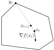
3.1.3 The Frank–Wolfe method

One drawback of projected gradient descent is the projection step: given a pointx0and a bodyK, finding the closest pointΠK(x0)might be computationally expensive. Instead, we can use a different rule, the Frank–Wolfemethod (also calledconditional gradient descent) [11], that implements each gradient step using linear optimization over the bodyK. Loosely, at each timestep we find the point inKthat is furthest from the current point in the direction of the negative gradient, and move a small distance towards it.

yt

xt

∇f(xt)

xt+1

Figure 2: The Frank–Wolfe Update.

Formally, the update rule for Frank–Wolfe method is simple:

yt←arg min

y∈K h∇t,yi,

xt+1←(1−ηt)xt+ηtyt. (3.13) Settingηt=1/(t+1)in hindsight will give the following result.

Theorem 3.6(Smooth functions: Frank–Wolfe). If f isβ-smooth, K is a convex body with diameter D:=maxx,y∈Kkx−yk, then the update rule (3.13) guarantees

f(xT)−f(x∗)≤β

D2(1+lnT)

2T .

Proof. We use the simplest potential function fromTheorem 3.1:

Φt =t·(f(xt)−f(x∗)), and hence the change in potential is again:

Φt+1−Φt = (t+1)(f(xt+1)−f(xt)) + (f(xt)−f(x∗)). (3.14) To bound the change in potential (3.14), we observe thatxt+1−xt =ηt(yt−xt).

f(xt+1)−f(xt)≤ h∇t,xt+1−xti+ β

2kxt+1−xtk

2

(by smoothness)

=ηth∇t,yt−xti+ β ηt2

2 kyt−xtk

≤ηth∇t,x∗−xti+ β η_t2

2 kyt−xtk

2

(by optimality ofyt) f(xt)−f(x∗)≤ h∇t,xt−x∗i. (by convexity) Settingηt :=1/(t+1)cancels the linear terms and hence the potential change (3.14) is at mostβ ηtD2/2. Summing overtand usingΦ0=0, the final potentialΦT ≤D2(1+lnT), and hence

f(xT)−f(x∗) =β

(1+lnT)·D2

2T .

We can remove the logarithmic dependence in the error by multiplying the potential by(t+1)as in Theorem 3.2; this gives the following theorem, whose simple proof we omit.

Theorem 3.7(Smooth functions: Frank–Wolfe, take II). If f is β-smooth, K is a convex body with D:=maxx,y∈Kkx−yk, then the update rule (3.13) withηt=2/(t+1)guarantees

f(xT)−f(x∗)≤2β D2 T+1.

3.2 Well-conditioned functions

If a function is bothα-strongly convex andβ-smooth, it must be thatα≤β. The ratioκ:=β/α is called thecondition numberof the convex function. We now show a much stronger convergence guarantee for “well-conditioned” functions, i. e., functions with smallκvalues. The update rule is the same as for smooth functions:

xt+1←xt− 1

β ∇t . (3.15)

Theorem 3.8(GD: Well-conditioned). Given a function f that is bothα-strongly convex andβ-smooth, defineκ:=β/α. The update rule (3.15) ensures

f(xT)−f(x∗)≤exp(−T/κ)·(f(x0)−f(x∗)) for all x∗.

Proof. We setγ=1/(κ−1)for brevity,1and use the potential

Φt= (1+γ)t·(f(xt)−f(x∗)) . (3.16) This is a natural potential to use, as we wish to show that f(xT)−f(x0)falls exponentially withT.

1_{Note that}

κ=1 iff f(x) =ax|x+b|x+cfor suitable scalarsa,candb∈Rn; in this case it is easily checked that the

The potential change. A little rearrangement gives us

Φt+1−Φt= (1+γ)t·

(1+γ) f(xt+1)−f(xt)

+γ f(xt)−f(x∗)

. (3.17)

We bound the two terms separately. Using the smoothness analysis from (3.5):

f(xt+1)−f(xt)≤ − 1 2βk∇tk

2_.

And by the definition of strong convexity,

f(xt)−f(x∗)≤ h∇t,xt−x∗i − α

2kxt−x

∗_k2_≤ 1

2αk∇tk

2

where the second inequality usesha,bi − kbk2_{/2≤ kak}2_{/2. Plugging this back into (3.17) gives}

(1+γ)t

−1+γ 2β +

γ 2α

k∇tk2

which is 0 by our choice ofγ. Hence, afterT steps,

f(xT)−f(x∗)≤(1+γ)−T(f(x0)−f(x∗)) = (1−1/κ)T(f(x0)−f(x∗))

≤e−T/κ_(f(x

0)−f(x∗)). (3.18)

Hence the proof.

Here we can show that the algorithm’s pointxT also gets rapidly closer tox∗. Ifx∗is the optimal point, we know∇f(x∗) =0. Now smoothness gives f(x0)−f(x∗)≤(β/2)kx0−x∗k2, and strong convexity

gives(α/2)kxT−x∗k2≤ f(xT)−f(x∗). Plugging into (3.18) gives us that kxT−x∗k2≤κe−T/κ· kx0−x∗k2.

A few remarks. Firstly,Theorem 3.8implies that reducing the error by a factor of 1/2 can be achieved by increasingT additivelybyκln 2. Hence if the condition numberκis constant, every constant number of rounds of gradient descent gives us one additional bit of accuracy! This behavior, where getting error bounded byεrequiresO(logε−1)steps, is calledlinear convergencein the numerical analysis literature.

One may ask if the convergence for smooth, and for well-conditioned functions is optimal as a function ofT. The answer is no: a famed result of Nesterov gives faster (and optimal) convergence rates. We see this result and a potential-function-based proof in §5.

Finally, the proof ofTheorem 3.8can be extended to the constrained case using the same potential function and the update rule (3.10), but now using an analog ofClaim 3.5that shows that for anyy∈K,

4

The mirror-descent framework

The gradient descent algorithms in the previous sections work by adding some multiple of the gradient to current point. However, this should strike the reader as somewhat strange, since the pointxt and the gradient∇f(xt)are objects that lie in different spaces and should be handled accordingly. In particular, if xt lies in some vector spaceE, the gradient∇f(xt)lies in the dual vector spaceE∗. (This did not matter earlier sinceRnequipped with the Euclidean norm is self-dual, but now we want to consider general norms and would like to be careful.)

A key insight of Nemirovski and Yudin [18] was that substantially more general and powerful results can be obtained, without much additional work, by considering these spaces separately. For example, it is well-known (and we will show) that the classic multiplicative-weights update method can be obtained as a special case of this general approach.

4.1 Basic mirror descent

The key idea in mirror descent is to define an injective mapping betweenE toE∗, which is called the mirror map. Given a pointxt, we first map it toE∗, make the gradient update there, and then use the inverse map back to obtain the pointxt+1.

We start some basic concepts and notation. Consider some vector spaceEwith an inner producth·,·i, and define a normk·konE. To measure distances inE∗, we use thedual normdefined as

kyk_∗:= max x:kxk=1

hx,yi. (4.1)

By definition we have

hx,yi ≤ kxk · kyk_∗, (4.2)

which is often referred to as thegeneralized Cauchy-Schwarzinequality. A functionhisα-strongly convexwith respect tok·kif

h(y)≥h(x) +h∇h(x),y−xi+α

2ky−xk

2_{. (4.3)}

Such a strongly convex functionhdefines a map fromEtoE∗via its gradient: indeed, the mapx7→∇h(x)

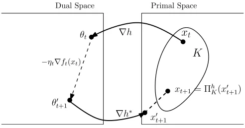
xt

∇h

θt

−ηt∇ft(xt)

θ0 t+1

x0 t+1

xt+1= ΠhK(x 0 t+1)

K

∇h∗

Dual Space Primal Space

Figure 3: Mirror Descent.

4.1.1 The update rules

Since∇h:E→E∗gives us a map from the primal spaceEto the dual spaceE∗, we keep track of the

image pointθt=∇h(xt)as well. Now, the updates are the natural ones, given by θt0+1=θt−ηt∇ft(xt),

x_t0₊₁=∇h∗(θt0+1),

xt+1=arg min

x∈KDh(xkx 0 t+1).

(4.4)

In other words, givenxt ∈E, we addηt times the negative gradient to its image θt =∇h(xt) in the dual space to getθ_t0₊₁, pull the result back tox_t0₊₁∈E (using the inverse mappingx_t0₊₁=∇h∗(θ_t0₊₁)), and project it back ontoKto getxt. Of course, we may not want to use the Euclidean distance for the projection; the “right” distance in this case is theBregman divergence Dh(ykx)fromxtoy, which we discuss shortly.

An equivalent way to present the mirror descent update is the following:

xt+1=arg min

x∈K

hηt∇ft(xt),x−xti+Dh(xkxt)

. (4.5)

This is a generalization of (2.2). The equivalence is easy to see in the unconstrained case (just take derivatives), for the constrained case one uses the KKT conditions.

4.1.2 Bregman divergences

Given a strictly convex functionh:Rd→R, define theBregman divergencefromxtoy Dh(ykx):=h(y)−h(x)− h∇h(x),y−xi

normk·k, thenDh(ykx)≥(β/2)ky−xk2. Also,Dh(ykx)is a convex function ofy(for a fixedx, this is a convex function minus a linear term), and the gradient of the divergence with respect to the first argument is∇y(Dh(ykx)) =∇h(y)−∇h(x).

For example, the functionh(x):= (1/2)kxk2₂is 1-strongly convex with respect to`2(and hence strictly

convex), and the associated Bregman divergenceDh(ykx) = (1/2)ky−xk2₂, half the squared`2distance.

This distance is not a metric, since it does not satisfy the triangle inequality. Or consider thenegative entropy function h(x):=∑ixilnxi defined on the probability simplex4n:={x∈[0,1]n|∑ixi =1}. Forx,y∈ 4n, the associated Bregman divergenceDh(ykx) is ∑iyiln(yi/xi), the relative entropy or Kullback-Leibler (KL) divergencefromxtoy. This distance is not even symmetric inxandy.

Bregman projection. Given a convex bodyKand a strictly convex functionh, we define theBregman projectionof a pointx0onKas

ΠhK(x0) =argminx∈KDh(xkx0).

Ifx0∈K, thenΠh_K(x0) =x0 becauseDh(x0kx0) =0. Forh(x) = (1/2)kxk2, this corresponds to the usual Euclidean projection. A very useful feature of Bregman projections is that they satisfy a “Pythagorean inequality” with respect to the divergence, analogous toFact 2.2.

Proposition 4.1(Generalized Pythagorean property). Given a convex body K⊆_Rn_{, let a∈K and b}0_∈ Rn. Let b=ΠhK(b0). Then

h∇h(b0)−∇h(b),a−bi ≤0.

In particular,

Dh(akb0)≥Dh(akb) +Dh(bkb0), (4.6) and hence Dh(akb)≤Dh(akb0).

Proof. Recall that for any convex functiongand convex bodyK, ifx∗=argmin_x∈Kg(x)is the minimizer ofginK, thenh∇g(x∗),y−x∗i ≥0 for ally∈K. Usingg(x) =Dh(xkb0), and noting thatg(x)is convex with∇g(x) =∇h(x)−∇h(b0)and that the minimizerx∗=b, we geth∇h(b)−∇h(b0),a−bi ≥0 for all

a∈K.

For the second part, expand the terms using the definition ofDh(akb)and cancel the common terms, the desired inequality turns out to be equivalent toh∇h(b0)−∇h(b),a−bi ≤0. The last inequality uses

that the divergences are non-negative.

4.1.3 The analysis

We consider the more generalonlineoptimization setting, and prove the following regret bound.

Theorem 4.2. Let K be a convex body, f₁, . . . ,fT be convex functions defined on K,k · kbe a norm, and h be anαh-strongly convex function with respect tok · k. The mirror descent algorithm starting at x0and

taking constant step sizeηt=ηin every iteration, produces x1, . . . ,xT such that T

∑

ft(xt)− n

∑

ft(x∗)≤

Dh(x∗kx0)

η +

η∑Tt=1k∇ft(xt)k2∗ 2αh

Proof. Define the potential

Φt =

Dh(x∗kxt)

η . (4.8)

Observe that plugging inh(x) = (1/2)kxk2₂gives us the potential function (2.3) for the Euclidean norm.

The potential change. For brevity, use∇t :=∇ft(xt). Dh(x∗kxt+1)−Dh(x∗kxt)

≤Dh(x∗kx0t+1)−Dh(x∗kxt) (generalized Pythagorean property)

=h(x∗)−h(x_t0₊₁)− h∇h(x0t+1)

| {z }

θ_t0+1

,x∗−x0_t+1i −h(x∗) +h(xt) +h∇h(xt)

| {z } θt

,x∗−xti

=h(xt)−h(xt0+1)− hθt0+1,xt−x0t+1i − hθt0+1−θt,x∗−xti

=h(xt)−h(x0t+1)− hθt,xt−x0t+1i

| {z }

strong convexity

+hηt∇t,xt−xt0+1i+hηt∇t,x∗−xti

≤ −αh 2 kx

0

t+1−xtk2+ηth∇t,xt−x0t+1i+ηth∇t,x∗−xti ≤ η

2

t 2αh

k∇tk2_∗+ηth∇t,x∗−xti. (4.9) The last inequality uses generalized Cauchy-Schwarz to getha,bi ≤ kbkkak∗≤ kbk2/2+kak2∗/2. Ob-serve that (4.9) precisely maps to (2.7) when we consider the Euclidean norm.

The amortized cost. Recall that we setηt =ηfor all steps. Hence, dividing (4.9) and substituting, ft(xt)−ft(x∗) + (Φt+1−Φt)≤ft(xt)−ft(x∗) +h∇t,x∗−xti

| {z }

≤0 by convexity offt

+ η

2αh k∇tk2∗.

The total regret then becomes

∑

(ft(xt)−ft(x∗))≤Φ0+

∑

t η 2αh

k∇tk2∗≤

Dh(x∗kx0)

η +

η∑Tt=1k∇tk2∗ 2αh

.

Hence the proof.

4.1.4 Special cases

To get some intuition, let us look at some well-known special cases. If we use the`2norm, andh(x):=

(1/2)kxk2₂ which is clearly 1-strongly convex with respect to`2, the associated Bregman divergence

Dh(x∗kx) = (1/2)kx∗−xk2₂. Moreover, the Euclidean norm is self-dual, so if we boundk∇ftk₂byG, the total regret bound above is

1 2ηkx

∗₋

This is the same result for projected gradient descent we derived inTheorem 2.1—and in fact the algorithm is also precisely the same.

Now consider the `1 norm, withK being the probability simplex 4n:={x∈[0,1]n|∑ixi =1}. If we choose the negative entropy functionh(x):=∑ixilnxi, thenDh(x∗kx) is just the well-known Kullback-Liebler divergence. Moreover, Pinsker’s inequality says thatKL(pkq)≥(1/2)kp−qk2<sub>1</sub>, which implies thathis 1-strongly convex with respect to`1. ApplyingTheorem 4.2now gives a regret bound of

KL(x∗kx0)

η +

η

2

∑

2

∞.

Let’s also see what the mirror descent algorithm does in this case. The mirror map takes the pointxto

∇h(x) = (1+logxi)i, and the inverse map takesθto∇h∗(θ) = (eθi−1)i. This point may be outside the probability simplex, so we do a Bregman projection, which in this case corresponds to just a rescaling x7→x/kxk₁. Unrolling the process, one can get a closed-form expression for the pointxT:

(xT)i=

(x0)i·exp{∑t(∇t)i}

∑j(x0)j·exp{∑t(∇t)j} .

For example, if we specialize even further to online linear optimization, where each function ft(x) =h`t,xifor some`t ∈[0,1]n, the gradient is`t and its`∞-norm isk`tk∞≤1, giving us the familiar

regret bound of

KL(x∗kx0)

η +

ηT 2

that we get from the multiplicative weights/Hedge algorithms. Which is not surprising, since this algorithm is precisely the Hedge algorithm!

4.2 An aside: Smooth functions and general norms

Let us consider minimizing a function that is smooth with respect to non-Euclidean norms, in the unconstrained case. When we consider an arbitrary normk·k, the definition of a smooth function (3.2) extends seamlessly. Now we can define an update rule by naturally extending (2.2):

xt+1←arg min

x

n1

2kx−xtk

2₊

ηth∇t,x−xti

o

, (4.10)

where the norm is no longer the Euclidean norm, but the norm in question. To evaluate the minimum on the right side, we can use basic Fenchel duality: given a functiong, its Fenchel dual is defined as

g?(θ):=max

z {hθ,zi −g(z)}.

If we defineg(z) = (1/2)kzk2, it is known thatg?(θ) = (1/2)kzk2_?(see [5, Example 3.27]). Hence

min x

n1

2kx−xtk

2₊

ηth∇t,x−xti

o

=−max x

n

ηth∇t,xt−xi − 1

2kxt−xk

=−max z

n

hηt∇t,zi − 1 2kzk

2o₌₋1

2kηt∇tk

2

?. (4.11) If a function f isβ-smooth with respect to the norm, then settingηt=1/β gives:

f(xt+1) (3.2)

≤ f(xt) +h∇t,xt+1−xti+ β

2kxt+1−xtk

2

= f(xt) +β

hηt∇t,xt+1−xti+ 1

2kxt+1−xtk

2_{= f(x}

t) +β·

−1 2kηt∇tk

2

?

,

where the last equality uses thatxt+1is the minimizer of the expression in (4.11). Summarizing, we get

f(xt+1)≤ f(xt)− 1 2βk∇tk

2

?. (4.12)

This is analogous to the expression (3.3). Now we can continue the proof as in §3.1, again defining D:=max{kx−x∗k | f(x)≤ f(x0)}, and using the generalized Cauchy-Schwarz inequality to get the

general-norm analog ofTheorem 3.2, due to Jaggi [14].

Theorem 4.3(GD: Smooth functions for general norms). Given a function f that is β-smooth with respect to the normk·k, the update rule (4.10) ensures

f(xT)−f(x∗)≤β 2D2

T+1.

5

Nesterov acceleration: A potential function proof

In §3, we proved a convergence rate of O(1/T) for smooth functions, using both projected gradient descent and the Frank–Wolfe method. But the lower bound is onlyΩ(1/T2). In this case, the algorithm

can be improved: Yurii Nesterov showed how to do it using hisaccelerated gradient descentmethods [19]. Recently there has been much interest in gaining a deeper understanding of this process, with proofs using “momentum” methods and continuous-time updates [29,24,17,30,8].

Let us now see potential-based proofs for his theorem, both for the smooth case, and for the well-conditioned case. We consider only the unconstrained case (i. e., whenK=Rn) and the Euclidean norm; the extension to general norms is sketched in §5.4.

5.1 An illustrative failed attempt

One way to motivate Nesterov’s accelerated algorithm is to revisit the proof for smooth functions in §3.1.1. Let us recall the essential facts. The potential was

Φt =t(f(xt)−f(x∗)) + a 2kxt−x

∗_k2

for somea>0. Hence the potential difference was:

Φt+1−Φt= (t+1) (f(xt+1)−f(xt))

| {z }

(3.5)

+f(xt)−f(x∗)

| {z }

(convexity)

+a

2 (kxt+1−x

∗_k2_{− kx}

t−x∗k2)

| {z }

≤(t+1)·

z }| {

− 1 2βk∇tk

2 2+

z }| {

h∇t,xt−x∗i+a

z }| {

ηth∇t,x∗−xti+η 2 t

2 k∇tk 2 2

=− t

2βk∇tk

2_≤0.

In that last expression we setηt=1/β anda=1/ηt=β to cancel the inner-product terms.

Observe that the potential may be decreasing considerably, by−t/(2β)· k∇tk2, but we are ignoring this large decrease. If we want to a show anO(1/t2)rate of convergence, a first (incorrect) attempt to get a better analysis would be to try to apply the analysis above with the potential changed to

Φt=t(t+1)(f(xt)−f(x∗)) + a 2kxt−x

∗_k2_.

In particular note the factorat =t(t+1)instead of(t+1)above. At first glance, the potential changeΦt+1−Φt would be

(t+2)(t+1)·(−₂1

βk∇tk

2 2)

| {z }

(3.5)

) +2(t+1)· h∇t,xt−x∗i+a ηth∇t,x∗−xti+η 2 t

2k∇tk 2 2

. (5.1)

Now if we change the step lengthηt from 1/β to something more aggressive, sayηt = (t+1)/(2β), and choosea=4β, the inner-product terms cancel, and the potential reduction seems to be at most

k∇tk2

−(t+1)(t+2)

2β +

(t+1)2

2β

≤0.

This would seem to give us anO(1/T2)convergence, with the standard update rule.

So where’s the mistake? It’s in our erroneous use of (3.5) in (5.1)—we used the cautious update withηt =1/β to get the first term of−1/(2β)· k∇tk2₂, but the aggressive update withηt= (t+1)(2β) elsewhere. To fix this, how about runningtwoprocesses, one cautious and one aggressive, and then combining them together linearly (with decreasing weight on the aggressive term) to get the new point xt? This is precisely what Nesterov’s Accelerated Method does; let’s see it now. (This is another way to arrive at the elegant linear-coupling view that Allen-Zhu and Orecchia present in [1].)

5.2 Getting the acceleration

As we just sketched, one way to view the accelerated gradient descent method is to run two iterative processes foryt andzt, and then combine them together to get the actual pointxt. The proof is almost the same as before.

The update steps. Start withx0=y0=z0. At timet, playxt. For brevity, define∇t :=∇f(xt). Now consider the update rules, where the color is used to emphasize the subtle differences (in particular,zis updated by the gradient atxin (5.3)):

yt+1←xt−_β1∇f(xt),

zt+1←zt−ηt∇f(xt),

xt+1←(1−τt+1)yt+1+τt+1zt+1.

The potential. This is the same one from the failed attempt:

Φ(t) =t(t+1)·(f(yt)−f(x∗)) +2β· kzt−x∗k2 . (5.5) The potential change. Define∆Φt =Φ(t+1)−Φ(t). By the standard GD analysis in (2.7),

1

2(kzt+1−x

∗_k2_{− kz}

t−x∗k2) = ηt2

2 k∇tk

2₊

ηth∇t,x∗−zti (5.6) implies that

∆Φt =t(t+1)·(f(yt+1)−f(yt)) +2(t+1)·(f(yt+1)−f(x∗)) +4β

η_t2 2 k∇tk

2₊

ηth∇t,x∗−zti

.

By smoothness and the update rule foryt+1, (3.5) implies

f(yt+1)≤ f(xt)−

1 2βk∇tk

2

.

Substituting, and noting 2β ηt2= (t+1)2/2β ≤(t+1)(t+2)/2β by the choice ofηt, the resulting (negative) squared-norm term can be dropped to give

∆Φt≤t(t+1)·(f(xt)−f(yt)) +2(t+1)·(f(xt)−f(x∗)) +4β ηth∇t,x∗−zti ≤t(t+1)· h∇t,xt−yti+2(t+1)· h∇t,xt−x∗i+2(t+1)· h∇t,x∗−zti

using convexity for the first two terms, andηt= (t+1)/2β for the last one. Collecting like terms,

∆Φt≤(t+1)· h∇t,(t+2)xt−tyt−2zti=0, (5.7) by using (5.4) andτt=2/(t+2). HenceΦt ≤Φ0for allt≥0. This proves:

Theorem 5.1(Accelerated GD). Given aβ-smooth function f , the update rules (5.2)-(5.4) ensure

f(yt)−f(x∗)≤2β

kz₀−x∗k2 t(t+1) .

5.2.1 An aside: Optimizing parameters and making connections

Suppose we choose the generic potential

Φ(t) =λt2−1(f(yt)−f(x∗)) + β 2kzt−x

∗_k2_,

whereλt=Θ(t2), and try to optimize the calculation above. Havingλt2−λt2−1=λt andτt=1/λt makes the calculations work out very cleanly. Solving this recurrence leads to the (somewhat exotic-looking) weights

λ0=0, λt = 1+

q

1+4λ_t2₋₁

used in the standard exposition ofAGM2.

The update rules (5.2)–(5.4) have sometimes been calledAGM2(Nesterov’s second accelerated method) in the literature. A different set of update rules (calledAGM1) are the following: for the optimized choice ofλt from (5.8), define:

yt+1←xt− 1

β∇f(xt), xt+1←

1−1−λt λt+1

yt+1+

1−λt λt+1

yt.

(5.9)

(5.10)

Let us show the simple equivalence (also found in, e. g., [27,9,16]).

Lemma 5.2.Using updates (5.9–5.10) and setting zt:=λtxt−(λt−1)yt=λt(xt−yt) +yt, andτt:=1/λt leads to the updates (5.2–5.4).

Proof. Clearlyyt is the same as above, so it suffices to show thatzt andxt behave identically. Indeed, rewriting the definition ofzt and substitutingτt=1/λt gives

xt = (1−τt)yt+τtzt,and

zt+1−zt = (λt+1(xt+1−yt+1) +yt+1)−(λt(xt−yt) +yt). (5.11) Moreover, rewriting (5.10) gives

λt+1(xt+1−yt+1)−(1−λt)(yt−yt+1) =0. (5.12)

Subtracting (5.12) from (5.11) gives

zt+1−zt=λtyt+1−λtxt =− λt

β∇f(xt). (5.13)

Recalling thatλt=1/τt = (β ηt), this is precisely the update rulezt+1←zt−ηt∇f(xt). This shows the equivalence of the two update rules.

5.3 The constrained case with acceleration

The update steps. The update rule is very similar to the one above, it just involves projecting the points onto the bodyK. Formally, again we start with x0=y0=z0. At timet, play xt. For brevity, define

∇t :=∇f(xt). Now consider the update rules, where again the color is used to emphasize the subtle differences:

yt+1←ΠK(xt−_β1∇f(xt)),

zt+1←ΠK(zt−ηt∇f(xt)),

xt+1←(1−τt+1)yt+1+τt+1zt+1.

(5.14) (5.15) (5.16) We now show that this update rule satisfies same guarantee as inTheorem 5.1for the unconstrained case.

Theorem 5.3(Accelerated GD). Given aβ-smooth function f , the update rules (5.14)-(5.16) ensure f(yt)−f(x∗)≤2β

kz0−x∗k2

The potential.

Φ(t) =t(t+1)·(f(yt)−f(x∗)) +2β· kzt−x∗k2 . (5.17) Change in potential.

Φt+1−Φt= (t+1)(t+2)(f(yt+1)−f(xt))

| {z }

(?)

−t(t+1)(f(yt)−f(xt)) +2(t+1)(f(xt)−f(x∗))

| {z }

(??)

+2β· kzt+1−x∗k2− kzt−x∗k2

| {z }

(???)

.

Using convexity on both differences in(??)gives

≤ −t(t+1)h∇t,yt−xti+2(t+1)h∇t,xt−x∗i

= (t+1)· h∇t,−t(yt−xt) +2(xt−x∗)i.

Now(1−τt)(yt−xt) =τt(xt−zt), and ifτt=2/(t+2), then we gett(yt−xt) =2(xt−zt), and hence

(??) =2(t+1)h∇t,zt−x∗i. (5.18) The expression(? ? ?)is

2β(hzt+1−zt,zt+1−x∗i − kzt+1−ztk2. By the Pythagorean property,hz0

t+1−zt+1,zt+1−x∗i ≥0 wherezt0+1=zt−ηt∇t. Settingηt = (t+1)/β and multiplying by 2β, adding to the term above,(? ? ?)is upper bounded by

−2(t+1)h∇t,zt+1−x∗i.

Combine with (5.18) to cancelx∗, it suffices to show the following claim:

Lemma 5.4.

(?)

z }| {

(t+1)(t+2)(f(yt+1)−f(xt)) +

(??)+(???)

z }| {

2(t+1)h∇t,zt−zt+1i − kzt+1−ztk2≤0. Proof. By smoothness,

f(yt+1)−f(xt)≤ h∇t,yt+1−xti+ β

2kyt+1−xtk

2_.

As

min y∈K

h∇t,y−xti+ β

2ky−xtk

2

in minimized by the definition ofyt+1, we get that for anyv∈K, the RHS is

≤ h∇t,v−xti+ β

2kv−xtk

2_.

Definev:= (1−τt)yt+τtzt+1∈K, sov−xt =τt(zt+1−zt). Substituting, we get f(yt+1)−f(xt)≤τth∇t,zt+1−zti+

τt2β

2 kzt+1−ztk

2_.

5.4 The extension to arbitrary norms

Given an arbitrary normk·k, the update rules now use the gradient descent update (4.10) for smooth functions for theyvariables, and the mirror descent update rules (4.4) for thezvariables:

yt+1←arg min

y

β

2ky−xtk

2_+h

∇f(xt),y−xti

,

zt+1←arg min

z

hηt∇f(xt),zi+Dh(zkzt)

,

xt+1←(1−τt+1)yt+1+τt+1zt+1.

(5.19)

Given the discussion in the preceding sections, the update rules are the natural ones: the first is the update (4.10) for smooth functions, and the second is the usual mirror descent update rule (4.5) for the strongly-convex functionh. The step size is now set to

ηt =

(t+1)αh 2β ,

whereαhis such thathisαh-strongly convex with respect tok·k. Then, the potential function becomes:

Φ(t) =t(t+1)·(f(yt)−f(x∗)) + 4β

αh

·Dh(x∗kzt), (5.20)

which on substitutingDh(x∗kzt) = (1/2)kx∗−ztk2andαh=1 gives (5.5).

We already have all the pieces to bound the change in potential. Use the mirror descent analysis (4.9) to get

Dh(x∗kzt+1)−Dh(x∗kzt)≤ η_t2 2αh

k∇tk2∗+ηth∇t,x∗−xti. which replaces (5.6). Infer

f(yt+1)≤f(xt)− 1 2βk∇tk

2

∗

from (4.12) in the smooth case. Substitute these into the analysis from §5.2(with minor changes for the αhterm) to get the following theorem:

Theorem 5.5(Accelerated GD: General norms). Given aβ-smooth function f with respect to normk·k, the update rules (5.19) ensure

f(yt)−f(x∗)≤ 4β αh

·Dh(x ∗_kz

0)−Dh(x∗kzt) t(t+1) .

5.5 Acceleration for strongly convex functions

Now consider the case when the function f is well-conditioned with condition numberκ =β/α, and describe the algorithm of Nesterov with convergence rate exp(−t/√κ) [20]. Again, this is the best possible for gradient methods.

Reduction from smooth case. Theorems5.1and5.3for the (constrained) smoothed case give that f(yt)−f(x∗)≤2β

kx₀−x∗|2

t(t+1) .

Together with strong convexity,

f(yt)−f(x∗)≥ α 2kyt−x

∗_k2_,

this giveskyt−x∗k2≤4κkx0−x∗k2/t(t+1).

So int=4√κ steps, the distancekyt−x∗kis at most half the initial distance kx0−x∗kfrom the

optimum. Starting the algorithm again withyt as the initial point, and iterating this process thus gives an overall algorithm, that intsteps has error at most 2−t/4

√

κ_kx−x

0k.

Restarting the algorithm after every few steps is not ideal, and we now describe Nesterov’s algorithm with this improved convergence rate. For simplicity only consider the unconstrained case.

The update rules. We now use the following updates (which look very much like theAGM1updates):

yt+1←xt− 1

β∇f(xt), xt+1←

1+

√ κ−1 √

κ+1

yt+1−

√ κ−1 √

κ+1yt.

(5.21)

(5.22)

For the analysis, it will be convenient to defineτ=1/( √

κ+1)and set

zt+1:=1_τ xt+1−1−_ττ yt+1. (5.23)

We now show that that the error aftertsteps is f(yt)−f(x∗)≤(1+γ)−t

α+β

2 kx0−x ∗_k2

, (5.24)

whereγ=1/( √

κ−1)(as in §3.2, forκ=1 the algorithm reaches optimum in a single step andy1=x∗,

and hence we assume thatκ>1). This improves on the error of

(1+1/κ)−tβ 2kx0−x

∗_k2

we get from §3.2.

The potential. Consider the potential

Φ(t) = (1+γ)t

f(yt)−f(x∗) + α

2kzt−x ∗_k2_.

Observe that

Φ0= f(y0)−f(x∗) +

α 2kz0−x

∗_k2_.

Asx0=y0=z0, and byβ-smoothness of f,

Φ0≤

α+β

Change in potential. To show the error bound (5.24), it suffices to show that∆Φ(t) =Φ(t+1)−Φ(t)≤

0 for eacht. This is equivalent to showing

(1+γ)(f(yt+1)−f(x∗))−(f(yt)−f(x∗)) + α

2 (1+γ)kzt+1−x

∗_k2_{− kz}

t−x∗k2

≤0.

We first bound the terms involving f in the most obvious way. As above, we use∇t as short-hand for

∇f(xt). Byβ-smoothness and the update rule, again f(yt+1)≤ f(xt)−

1 2βk∇tk

2_.

So,

(1+γ)(f(yt+1)−f(x∗))−(f(yt)−f(x∗))

≤ f(xt)−f(yt) +γ(f(xt)−f(x∗))−(1+γ) 1 2βk∇tk

2

≤ h∇t,xt−yti+γ

h∇t,xt−x∗i − α

2kxt−x ∗_k2

−1+γ 2β k∇tk

2_{, (5.25)}

where the last inequality used convexity and strong convexity respectively. We now want to remove references toyt. By definition (5.23),

zt=

1 τ−1

(xt−yt) +xt = √

κ(xt−yt) +xt, so we inferγ(zt−x∗) =

√

κ γ(xt−yt) +γ(xt−x∗). Using √

κ γ=1+γ, simple algebra gives

(xt−yt) +γ(xt−x∗) = 1

1+γ γ(zt−x ∗

) +γ2(xt−x∗)

.

For brevity we useXt:=xt−x∗,Zt =zt−x∗, and substitute the above expression into (5.25) to get 1

1+γh∇t,γZt+γ

2_X

ti − α γ

2 kXtk

2₋1+γ

2β k∇tk

2_{. (5.26)}

Now, let us upper bound the terms in∆Φ(t)involvingz. Conveniently, we can relatezt+1andzt using a simple calculation that we defer for the moment.

Claim 5.6. zt+1= (1−√1_κ)zt+√1_κxt−_α√1_κ∇t and so zt+1−x∗=₁₊1_γZt+₁₊γ_γXt−_α(1γ_+γ)∇t.

Now useClaim 5.6and expand usingka+b+ck2=kak2+kbk2+kck2+2ha,bi+2hb,ci+2ha,ci:

(1+γ)kzt+1−x∗k2− kzt−x∗k2

= 1

1+γ

kZtk2+γ2kXtk2+ γ2 α2

k∇tk2+2γhZt,Xti − 2γ

α

h∇t,Zti − 2γ2

α

h∇t,Xti

Now sum (5.26) andα/2 times (5.27). The terms involvingk∇tk2cancel since 1+γ

2β =

α γ2 2α2_(1+γ)

(by the definition ofγ). Moreover, the inner-product terms involving∇t also cancel. Hence the potential change is at most

∆Φ(t)≤α γ

2 kXtk

2

−1+ γ

1+γ

+α

2kZtk

2

1 1+γ −1

+ α γ

1+γhZt,Xti

=− α γ 2(1+γ)

kXtk2+kZtk2−2hZt,Xti

(5.28)

=− α γ

2(1+γ)kZt−Xtk

2_{≤0. (5.29)}

Hence the potential does not increase, as claimed. It only remains to proveClaim 5.6.

Proof ofClaim 5.6. The expression of xt+1 from (5.22) can be written as (2−2τ)yt+1−(1−2τ)yt. Plugging into the expression forzt+1from (5.23) gives

zt+1=

1

τ((2−2τ)yt+1−(1−2τ)yt−(1−τ)yt+1)

=1

τ((1−τ)yt+1−(1−2τ)yt).

Using the update rule (5.21) foryt+1, and the relationxt = (1−τ)yt+τzt to eliminateyt

=1

τ

(1−τ)

xt− 1 β∇t

−(1−2τ)

1−τ (xt−τzt)

=1−2τ

1−τ zt+ τ 1−τxt−

1−τ τ β ∇t.

Usingτ=1/( √

κ+1)andβ=κ αnow gives the claim.

Acknowledgments

We thank the referees and Laci Babai for their detailed and thoughtful feedback that helped improve the presentation substantially. We also thank Sébastien Bubeck, Daniel Dadush, Jelena Diakonikolas, Nick Harvey, Elad Hazan, Greg Koumoutsos, Raghu Meka, Aryan Mokhtari, Marco Molinaro, Thomas Rothvoß, and Kunal Talwar for their helpful comments.

References

[2] AMIRBECK ANDMARCTEBOULLE: Mirror descent and nonlinear projected subgradient methods for convex optimization.Oper. Res. Lett., 31(3):167–175, 2003. [doi:10.1016/S0167-6377(02)00231-6] 16

[3] AHARON BEN-TAL AND ARKADI NEMIROVSKI: Lectures on Modern Convex Optimization. Society for Industrial and Applied Mathematics, 2001. [doi:10.1137/1.9780898718829] 3

[4] DMITRIP. BERTSEKAS, ANGELIANEDI ´C,ANDASUMANE. OZDAGLAR:Convex Analysis and Optimization. Athena Scientific, 2003. 16

[5] STEPHEN BOYD ANDLIEVENVANDENBERGHE:Convex Optimization. Cambridge University Press, 2004. [doi:10.1017/CBO9780511804441] 20

[6] SÉBASTIENBUBECK: Convex optimization: algorithms and complexity. Foundations and Trends in Machine Learning, 8(3-4):231–357, 2015. [doi:10.1561/2200000050,arXiv:1405.4980] 3,6 [7] NICOLÒCESA-BIANCHI AND GÁBORLUGOSI:Prediction, Learning, and Games. Cambridge

University Press, Cambridge, 2006. 3,9

[8] JELENADIAKONIKOLAS AND LORENZO ORECCHIA: The approximate gap technique: a uni-fied approach to optimal first-order methods. SIAM J. Optim., 29(1):660–689, 2019. SIAM. [arXiv:1712.02485] 2,3,21

[9] YOELDRORI AND MARC TEBOULLE: Performance of first-order methods for smooth convex minimization: a novel approach. Math. Program., 145(1-2):451–482, 2014. [doi:10.1007/s10107-013-0653-0,arXiv:1206.3209] 24

[10] JOHNC. DUCHI: Introductory Lectures on Stochastic Optimization, 2016. Available atauthor’s webpage. 3

[11] MARGUERITE FRANK AND PHILIP WOLFE: An algorithm for quadratic programming. Naval Research Logistics Quarterly, 3(1-2):95–110, 1956. [doi:10.1002/nav.3800030109] 13

[12] ELADHAZAN: Introduction to online convex optimization.Foundations and Trends in Optimization, 2(3-4):157–325, 2016. [doi:10.1561/2400000013] 3

[13] JEAN-BAPTISTE HIRIART-URRUTY AND CLAUDE LEMARÉCHAL: Fundamentals of Convex Analysis. Springer, 2001. [doi:10.1007/978-3-642-56468-0] 2

[14] MARTINJAGGI: Revisiting Frank–Wolfe: projection-free sparse convex optimization. InProc. 13th Internat. Conf. on Machine Learning (ICML’13), pp. 427–435, 2013. [PMLR]. 21

[15] SAHARKARIMI ANDSTEPHENA. VAVASIS: A single potential governing convergence of conju-gate gradient, accelerated gradient and geometric descent, 2017. [arXiv:1712.09498] 3

[17] WALID KRICHENE, ALEXANDREM. BAYEN, ANDPETERL. BARTLETT: Accelerated mirror descent in continuous and discrete time. InAdv. in Neural Inform. Processing Systems 28 (NIPS’15), pp. 2845–2853, 2015. NIPS. 2,3,21

[18] ARKADISEMËNOVICHNEMIROVSKI ANDDAVIDBERKOVICHYUDIN: Problem Complexity and Method Efficiency in Optimization. John Wiley & Sons, Inc., 1983. 2,3,16

[19] YURIINESTEROV: A method of solving a convex programming problem with convergence rate O(1/k2). Soviet Mathematics Doklady, 27:372–376, 1983. LINK at Math-Net.ru. 21

[20] YURII NESTEROV: Introductory Lectures on Convex Optimization – A Basic Course. Kluwer Academic Publishers, 2004. [doi:10.1007/978-1-4419-8853-9] 3,6,26

[21] JAVIER PEÑA: Convergence of first-order methods via the convex conjugate. Oper. Res. Lett., 45(6):561–564, 2017. [doi:10.1016/j.orl.2017.08.013,arXiv:1707.09084] 3

[22] SHAI SHALEV-SHWARTZ: Online learning and online convex optimization. Foundations and Trends in Machine Learning, 4(2):107–194, 2012. [doi:10.1561/2200000018] 3

[23] NAUMZUSELEVICHSHOR:Minimization Methods for Non-differentiable Functions. Springer, 1985. [doi:10.1007/978-3-642-82118-9] 3

[24] WEIJIESU, STEPHENBOYD,ANDEMMANUELJ. CANDÈS: A differential equation for model-ing Nesterov’s accelerated gradient method: theory and insights. J. Mach. Learn. Res. (JMLR), 17(153):1–43, 2016. 2,3,21

[25] EIJI TAKIMOTO AND MANFRED K. WARMUTH: The minimax strategy for Gaussian density estimation. InProc. 13th Ann. Conf. on Computational Learning Theory (COLT’00), pp. 100–106. Morgan Kaufmann Publ., 2000. ACM DL. 8

[26] ADRIEN TAYLOR AND FRANCIS BACH: Stochastic first-order methods: non-asymptotic and computer-aided analyses via potential functions. In Proc. 32th Ann. Conf. on Computational Learning Theory (COLT’19), pp. 2934–2992. MLR Press, 2019. [PMLR]. [arXiv:1902.00947] 3 [27] PAULTSENG: On accelerated proximal gradient methods for convex-concave optimization, 2008.

Available atauthor’s webpage. 24

[28] NISHEETH K. VISHNOI: A mini-course on convex optimization, 2018. Available at author’s webpage. 3

[29] ANDREWIBISONO, ASHIAC. WILSON,AND MICHAELI. JORDAN: A variational perspective on accelerated methods in optimization. Proc. Natl. Acad. Sci. USA, 113(47):E7351–E7358, 2016. [doi:10.1073/pnas.1614734113,arXiv:1603.04245] 2,3,21

AUTHORS

Nikhil Bansal Researcher

Centrum voor Wiskunde en Informatica Amsterdam

The Netherlands bansal gmail com

http://www.win.tue.nl/~nikhil

Anupam Gupta Professor

Computer Science Department Carnegie Mellon University Pittsburgh, PA, USA anupamg cs cmu edu

http://www.cs.cmu.edu/~anupamg

ABOUT THE AUTHORS

NIKHILBANSALis a researcher at theCentrum voor Wiskunde en Informatica, Amsterdam. He attended theIndian Institute of Technology, Mumbaifor his B. Tech. degree, and received his Ph. D. fromCarnegie Mellon University, where he was advised byAvrim Blum. He got fascinated by algorithms after taking an undergraduate class byProf. Ajit A. Diwan. Since then he has enjoyed thinking about various kinds of algorithmic questions.