A Vision based Vehicle Detection System
Himanshu Chandel
Bahra University
Bahra University, National Highway 22, Waknaghat, Himachal Pradesh, 173234
Sonia Vatta
Bahra University
Bahra University, National Highway 22, Waknaghat, Himachal Pradesh, 173234
ABSTRACT
In recent years, automotive manufacturers have equipped their vehicles with innovative Advanced Driver Assistance Systems (ADAS) to ease driving and avoid dangerous situations, such as unintended lane departures or collisions with other road users, like vehicles and pedestrians. To this end, ADAS at the cutting edge are equipped with cameras to sense the vehicle surrounding. This research work investigates the techniques for monocular vision based vehicle detection. A system that can robustly detect and track vehicles in images. The system consists of three major modules: shape analysis based on Histogram of oriented gradient (HOG) is used as the main feature descriptor, a machine learning part based on support vector machine (SVM) for vehicle verification, lastly a technique is applied for texture analysis by applying the concept of gray level co-occurrence matrix (GLCM). More specifically, we are interested in detection of cars from different camera viewpoints, diverse lightning conditions majorly images in sunlight, night, rain, normal day light, low light and further handling the occlusion. The images has been pre-processed at the first step to get the optimum results in all the conditions. Experiments have been conducted on large numbers of car images with different angles. For car images the classifier contains 4 classes of images with the combination of positive and negative images, the test and train segments. Due to length of long feature vector we have deduced it using different cell sizes for more accuracy and efficiency. Results will be presented and future work will be discussed.
General Terms
Texture analysis, shape analysis, vision based systems
Keywords
Vision, texture, vehicle, car, autonomous, shape
1.
INTRODUCTION
Advanced driver assistance systems (ADAS) are technologies that provide a driver with essential information, automate difficult or repetitive tasks, and lead to an overall increase in car safety for everyone. Some of these technologies have been around for a long time, and they have already proven to result in an improved driving experience and better overall road safety. In recent years, there has been a significant increase in the number of the embedded electronic processors in automobiles from 1% in 1980 to over 22% in 2007 [1]. Among the different embedded sub-systems, vision-based advanced driver assistance systems (ADAS) are becoming more popular in recent times because of the availability of low-cost, high-resolution and pervasive cameras [2]. In order to meet the increasing demand in vision-based ADAS, manufacturers such as Texas Instruments etc. are releasing newer embedded platforms that are specifically catered for implementing vision algorithms in automobiles [3].
Navigation systems are used in a wide range of applications such as: Automotive Navigations System, Marine Navigation System, Global Positioning System, Surgical Navigation System, Inertial Guidance system and Robotic mapping.in addition to navigation systems advance driver assistance system is there to maintain safe speed, driving within lane, collision avoidance and at last reducing the severity of accident. There are a wide range of issues and difficult tasks in the domain of navigation systems such as complex backgrounds, low-visibility, weather conditions, cast shadows, strong headlights, direct sunlight during dusk and dawn, uneven street illumination and the problem of occlusions on which this thesis is concentrating. In modest term 4 levels should be accomplished to make a robust navigation system: detection, localization, recognition and understanding. In this research work a number of experiments were carried out on different real world data sets for evaluation and analysis of the methods applied to obtain the best results for detecting vehicles. In the field of surveillance, autonomous navigation, scene understanding occlusion is one of the most common problem and due to this problem lots of vision based algorithms lacks in robustness.
The problem of occlusion is commonly defined under object tracking and object detection. The results are obtained by using the shape features with Histogram of orientation gradient and calculating the texture features such as: entropy, contrast, correlation, homogeneity and energy.
By implementing gray level co-occurrence matrix. Further the training of the features data set is done by support vector machines using statistica and results are obtained on the rate of car detection on different datasets. The dataset which we used in the experiment is collected online by utilizing the images of size 64*64 pixels with positive and negative samples that is car and non-car images which includes occluded samples. The feature vector window with cell size of 3*3 is used for histogram of orientation gradients on the images with the output of feature vector with 1*14400, secondly to minimize the feature vector rather using principal component analysis or any other technique we implemented the window size of 32 * 32 to get the feature vector of length 1*144. Texture is also one of the important part in a biological vision system, the concept of gray level co-occurrence matrix is used, further concatenating the feature vector on the basis of entropy, contrast, correlation, homogeneity and energy with 3 different colour channels red, green and blue. The concatenation of feature vector finally, gives us the feature vector which is further classified and tested on the basis of support vector machines using Statistica. The dataset has been trained and tested using support vector machines with 2 different kernel types: RBF and linear. The overall results has been presented with more than 90% of accuracy rate in the overall system.
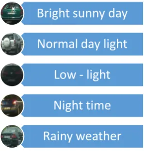
samples of car and non-car. The application of scene understanding and navigation systems various problems such as different light conditions, weather conditions, occlusions and illusions. In this thesis we performed the experiments on the given dataset which involves images under 6 different categories as shown in the Figure 3.1. The 6th category is occlusion, as all the images in the following categories have 25% of occluded image samples with partial and self-occlusion.
Fig 1: Dataset used
2.
LITERATURE REVIEW
In computer vision, the higher level of understanding with the camera as a sensor involves the tasks such as: place recognition, scene understanding, object detection, object categorization and action recognition. Many existing vision-based systems are not able of providing detailed information on individual vehicles but are limited to measure or quantify the traffic flow only, or to solve specific sub-problems (e.g. queue detection, inductive loop emulation, congestion detection on highways), lacking generality. Traffic control should be performed in different environment, weather and light conditions, with the capability of handling occlusions and illusions as well, in addition, urban scenes are particularly complex since the background condition is highly variable. The human perception is yet very intelligent as compared to machines, lots of research is going to make the real world applications by which it will be possible to give a vision to machines. Wide range of applications are there in the field of computer vision such as: Unmanned Aerial Vehicles (UAV’s), Unmanned Ground Vehicles (UGV’s), Unmanned underwater vehicles (UUv’s),Advanced driver assistance systems (ADAS), Automated visual Traffic Surveillance (AVTS), Autonomous Navigation, Pedestrian Classification, Scene Understanding. In computer vision the sensor we use is camera, to give vision to machines researchers work commonly on two platforms: monocular [4] or binocular (stereo) [5] vision. Now, the concept comes what is the difference between one image of a scene and on the other hand two image of the same scene taken from different viewpoints. The two images let us infer the depth information by means of geometry, with the help of triangulation technique [6].
Object tracking and detection is a classical research area in the field of computer vision from decades. Numerous kinds of applications are dependent on the area of object detection, such as advance driving assistance system, traffic surveillance, scene understanding, autonomous navigation etc. Many challenges still exist while detecting an object such as
illusion, low visibility, cast shadows and most importantly occlusions of object. Due to increase of traffic on roads, intelligent traffic surveillance systems are being implemented in various countries for highway monitoring and city road management system. Traditionally, shadow detection techniques have been employed for removing shadows from the background and foreground, but Sadeghi & Fathy used it as a novel feature for vehicles detection and occlusion handling. They have used photometric characteristic of darkest pixels of strong shadows in traffic images for occlusion handling. Multilevel framework is adopted by Zhang, Jonathan Wu, Yang and Wang for handling car occlusion in traffic; firstly occlusion is detected by evaluating the compactness ratio and interior distance ratio of vehicles, and then the detected occlusion is handled by removing a cutting region of occluded vehicles. On interframe level, occlusion is detected by performing subtractive clustering on the motion vectors of vehicle. Next comes the tracking level, occluded vehicles are tracked by using a bidirectional occlusion reasoning mechanism [7]. The more literature review is presented by Chandel, Vatta for the same purpose of vehicle detection under occlusions [8]. During literature review we came across a wide range of techniques and algorithms but here we will be focusing on the impactful algorithms given in the below Fig 1.
Fig 2: Important and reviewed techniques / algorithms
Vehicles may vary in shape, size, colour and appearance depending on pose. In order to solve the problem of vehicle detection various natural conditions we utilized the techniques based on shape and texture analysis.
2.1
Slam – Simultaneous Localization and
Mapping
SLAM can be implemented in many ways. First of all there is a huge amount of different hardware that can be used. Secondly SLAM is more like a concept than a single algorithm. There are many steps involved in SLAM and these different steps can be implemented using a number of different algorithms. SLAM consists of multiple parts; Landmark extraction, data association, state estimation, state update and landmark update. There are many ways to solve each of the smaller parts. It is a process by a mobile device or a robot builds the map of an environment and uses this map at the same time to deduce its location in it. The SLAM is commonly used for the robot navigation systems in an unknown environment, it’s more like a concept than a single algorithm. The first step in the SLAM process is to obtain data about the surroundings of the robot. Extended Kalman filter, a traditional approach is also quite often used for the estimation in robotics. While in SLAM during robot navigation in an environment the robot localize itself using maps. It is basically concerned with a problem of building a map of an unknown environment by a mobile robot while at the same
Bright sunny day
Normal day light
Low - light
Night time
time navigating the environment using the map. SLAM consists of multiple parts; Landmark extraction, data association, state estimation, state update and landmark update. The SLAM is based on Extended Kalman filter which utilizes the a priori map of the locations. The objective of the SLAM problem is to estimate the position and orientation of the robot together with the locations of all the features. SLAM is frequently used in Autonomous underwater vehicles, unmanned aerial vehicles and autonomous ground vehicles [9].
2.2
Surf – Speeded Up Robust Features
Speeded up robust features (SURF), is inspired by Scale Invariant feature transform (SIFT), it is a local feature detector and descriptor that can be used for tasks such as object recognition or 3D reconstruction. The basic version of SURF is several times faster than SIFT and is much more robust. The algorithm works on interest point detection, local neighborhood description and matching. SURF uses wavelet responses in horizontal and vertical direction for a neighborhood pixels. The surf algorithm is based on two basic steps feature detection and description. The detection of features in SURF relies on a scale-space representation, combined with first and second order differential operators. The originality of the SURF algorithm (Speeded up Robust Features) is that these operations are speeded up by the use of box filters techniques[10].
2.3
Dpm – Deformable Part Based Model
Deformable part based model is based on an object category that represents the appearance of the parts and how they relate to each other. The part is any element of an object or scene that can be reliably detected using only local image evidence. In part based model, each part represents local visual properties. The basic idea behind deformable parts is to represent an object model using a lower resolution root template and set a spatially flexible high resolution part templates. Deformable part based model is the next revolutionary idea after the Histogram of orientation gradient in object detection. Threshold employed in the deformable part based model in the non-maximum suppression filter is the key root of this algorithm. Lower the threshold, higher the number of detection [11].
3.
SHAPE ANALYSIS
The shape can be thought of as a silhouette of the object (e.g. obtained by illuminating the object by an infinitely distant light source). There are many applications where image analysis can be reduced to the analysis of shapes (e.g. organs, cells, machine parts, characters). Shape analysis methods play an important role in systems for object recognition, matching, registration, and analysis. The goal of shape analysis is to provide a simplified representation of the original shape so that the important characteristics of the shape are preserved. The work important in the above sentence may have different meanings in different applications. This general definition implies that the result of analysis can be either numeric (e.g. a vector) or non-numeric (e.g. a graph). The input to shape analysis algorithms are shapes (i.e. binary images). Research in shape analysis has been motivated, in part, by studies of the human visual form perception system. Methods for shape analysis are divided into several groups. Classification is done according to the use of shape boundary or interior and according to the type of result. Four resulting combinations are boundary scalar, boundary space domain, global scalar, and global space-domain methods. The last few decades have
resulted in an enormous amount of work related to shape analysis. As a kind of global shape description, shape analysis in transform domains takes the whole shape as the shape representation.
Generally, low level features such as colour, texture, shape, corner, etc., are used to represent the approximate perceptual representation of an image, using which similarity and dissimilarity of the images are computed. But it is found that the perceptual representation of an image in terms of low level features fails to capture entire semantic information of an image and it is often difficult to model accurately.
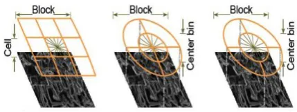
In this work The Histogram of oriented gradient [12] approach is utilized first to figure out the best features. It operates on a dense grid of uniformly spaced cells and used in local contrast normalization on overlapping blocks for improved accuracy. Basic idea behind HOG is that the appearance and shapes of local objects within an image can be well described by the distribution of intensity gradients as the votes for dominant edge directions. Such descriptor can be obtained by first dividing the image into small contiguous regions of equal size, called cells, then collecting histogram of gradients directions for the pixels with each cell and at last combining all these histograms. In order to improve the detection accuracy against varied illumination and shadowing, local contrast normalization can be applied by computing a measure of the intensity across larger region of image, called a block and using resultant value to normalize all cells within the block. There are 2 basic variants of HOG descriptors commonly used: Rectangular and Circular HOG.
Fig 3: Variants of HOG descriptors. (a) A rectangular HOG (R-HOG) descriptor with 3 × 3 blocks of cells. (b) Circular HOG (C-HOG) descriptor with the central cell divided into angular sectors as in shape contexts. (c) A
C-HOG descriptor with a single central cell.
The process starts from computation of image gradients, this is done by applying 1D centered, point discrete derivative mask in both the horizontal and vertical directions, which in specific are filter kernels of following form.
[-1, 0, 1] and
There are many more complex masks, such as sobel, prewitt, canny or diagonal mask, but these mask result in poorer performance. Then magnitude and orientation at each pixel I(x, y) is calculated by:
Θ (
) = arc tan
+
channel with the largest magnitude gives the pixels dominant magnitude and orientation.
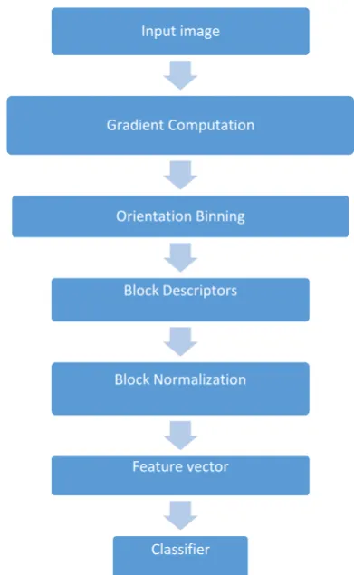
Step 1: Input image
In the first images are firstly pre-processed on the basis of size to get the optimum and best features in the feature vector queue. The operations were performed on the image size of 64*64 pixels.
Step 2: Gradient calculation
Magnitude and orientation at each pixel is calculated, with the gradient values at each pixel in x and y directions. In the samples, which we used, the largest magnitude gives the pixel dominant magnitude and direction.
Step 3: Orientation binning and normalization
Histograms of each cell are created. Every histogram bin has a spread of 20°. Every pixel in the cell casts a weighted voting into one of the 9 histogram bins that its orientation belongs to (0° - 180° = 90°). After block normalization the feature vector is calculated which contains the elements of the normalized cell histograms from all of the block regions. The slope is checked also called as orientation gradient and it is put in a bin. Then another region is sampled until entire image been sampled. Finally, with the help of slopes edges are determined.
Step 4: Block normalization and descriptors
Histograms are also normalized based on their energy (regularized L2 norm) across blocks. During the basic testing the blocks have a step size of 1 cell, a cell will be part of 4 blocks. This defines four differently normalized versions of the cell's histogram. These 4 histograms are concatenated to get the descriptor for the cell. After block normalization the feature vector is calculated which contains the elements of the normalized cell histograms from all of the block regions.
Step 5: Feature vector
Finally, to minimize the feature vector rather using principal component analysis or any other technique we implemented the window size of 32 * 32 to get the feature vector of length 1*144.
Fig 4: Overall flow of the technique for shape analysis
4.
TEXTURE ANALYSIS
Texture is an important cue for biological vision systems to estimate the boundaries of objects. Also, texture gradient is used to estimate the orientation of surfaces. For example, on a perfect lawn the grass texture is the same everywhere. However, the further away we look, the finer this texture becomes – this change is called texture gradient. For the same reasons, texture is also a useful feature for computer vision systems.
Gray level co-occurrence matrix is computed, firstly we separated the intensity in the image into a small number of different levels. Normalization of the matrix is done by determining the sum across all entries and dividing each entry by this sum. This co-occurrence matrix contains important information about the texture in the examined area of the image. The GLCM is created from a gray The GLCM is created from a gray-scale image.
We calculated and examined the following parameters for Red, Green and Blue colour channels.
b a
b
a
P
, 2
)
,
(
Energy
b a
b
a
P
b
a
P
,
2
(
,
)
log
)
,
(
Entropy
b a
b
a
P
b
a
,
1
2,
usually
,
)
,
(
|
|
Contrast
Input image
Gradient Computation
Orientation Binning
Block Descriptors
Block Normalization
Feature vector
y x b
a
y x
b
a
P
ab
,)
,
(
)
(
n
Correlatio
|
|
1
)
,
(
y
Homogeneit
b
a
b
a
P
5.
CLASSIFIER
A support vector machine is a classifier defined separating a hyper plane. SVM’s belong to a family of generalized linear classifiers. The foundations of Support Vector Machines (SVM) have been developed by Vapnik [13] and gained popularity due to many promising features such as better empirical performance. SVMs are commonly used to solve the classification problem. SVM is a useful technique for data classification. A classification task usually involves with training and testing data which consist of some data instances [14].
SVM is related to statistical learning theory which was first introduced in 1992. SVM becomes popular because of its success in handwritten digit recognition. It is now regarded as an important example of “kernel methods”, one of the key area in machine learning. In this thesis we are using 1 D feature vector for the classification problem of cars and non – car.
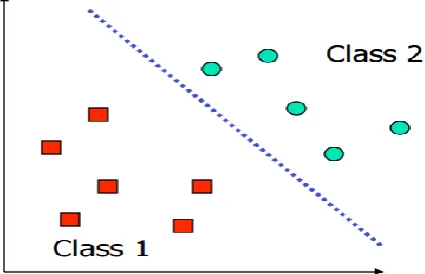
Each instance in the training set contains one target values and several attributes. The goal of SVM is to produce a model which predicts target value of data instances in the testing set which are given only the attributes [15]. Classification in SVM is an example of Supervised Learning. Known labels help indicate whether the system is performing in a right way or not. This information points to a desired response, validating the accuracy of thesystem, or be used to help the system learn to act correctly. A step in SVM classification involves identification as which are intimately connected to the known classes. This is called feature selection or feature extraction. Feature selection and SVM classification together have a use even when prediction of unknown samples is not necessary. They can be used to identify key sets which are involved in whatever processes distinguish the classes [16]. Support vector machines are used to identify the 2 classes, as in this thesis we are using car and non-car. A good decision boundary is a key for this algorithm. Consider a 2 classes such as car and non- car, which is a linearly separable classification problem. As defined in the Fig 5, we used class 1 as car and class 2 as non – car.
Fig 5: Linearly separable classification
6.
RESULTS
Our method was tested on a number of challenging sequences .The resolution of the images used for testing was 64 × 64 pixels. The algorithm has been developed using Matlab and for training purpose Statistica is used. The algorithm is run on an Intel Core I5, 3.00 GHz machine.
This section presents the experimental results obtained using a trained and testing model. The first one, based on the method suggested by [17] builds the appearance model based on shape feature vector and normalizing the histograms based on gradient. The feature vector of Gray level co-occurrence matrix based on 3 different colour channels, Red, Green and Blue. The Entropy, Contrast, Correlation, Energy and Homogeneity are calculated for each image to get the best results using texture and shape features.
The histogram of orientation gradient is implemented with the 20 * 20 cell size, to collect the best feature vector. The classification is performed using Statistica and implementing Support vector Machines (SVM).
Handling occlusion was one of the most critical parts in this work. Vehicle tend to be on roads and in different traffic conditions so the chances of occluding one car with another are high further depending on self-occlusion, as camera viewpoint angle is different . To solve this problem, some methods try to position the camera in the ceiling or at a vertical angle in the hopes of decreasing the chances of occlusion in surveillance systems. Although the vertical angle of a camera can solve occlusion problems, it is not applicable in all potential uses of vehicle tracking. The texture analysis gave us the optimum results for handling occlusion and with both shape and texture features, we were able to get the accuracy of more than 90% in both the conditions of real world scenarios.
6.1
Low light conditions
In case 1 that is 6.1 we present the natural condition of low light with the basic sample of dataset and results.
Fig 6: Sample of low light condition dataset
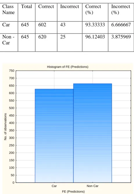
Case 1.1 Kernel Type – RBF
Table 1. Classification Summary – Support Vector Machine
Class Name
Total Correct Incorrect Correct (%)
Incorrect (%)
Car 645 602 43 93.33333 6.666667
Non - Car
645 620 25 96.12403 3.875969
Histogram of FE (Predictions)
Car Non Car
FE (Predictions) 0
50 100 150 200 250 300 350 400 450 500 550 600 650 700 750
N
o
.
o
f ob
se
rva
tio
n
s
Fig 8: Histogram of observed dataset
Case 1.2 Kernel Type – Linear
Table 2. Classification Summary – Support Vector Machine
Class Name
Total Correct Incorrect Correct (%)
Incorrect (%)
Car 645 591 54 91.62791 8.372093
Non - Car
645 605 40 93.79845 6.201550
Histogram of FE (Predictions)
Car Non Car
FE (Predictions) 0
50 100 150 200 250 300 350 400 450 500 550 600 650 700 750
N
o
.
o
f ob
se
rva
tio
n
s
Fig 9: Histogram of observed dataset
Fig 10: Overall performance of detector
6.2
Night conditions
In case 2 that is 6.2 we present the natural condition of night time with the basic sample of dataset and results.
Fig 11: Sample of night condition dataset
Case 2.1 Kernel Type – RBF
Table 3. Classification Summary – Support Vector Machine
Class Name
Total Correct Incorrect Correct (%)
Incorrect (%)
Car 70 70 0 100.00 0.00
Non - Car
Histogram of FE (Predictions)
Car Non Car
FE (Predictions) 0
5 10 15 20 25 30 35 40 45 50 55 60 65 70 75 80
N
o
.
o
f
o
b
s
e
rv
a
ti
o
n
s
Fig 12: Histogram of observed dataset
Fig 13: Overall performance of detector
Case 2.2 Kernel Type – Linear
Table 4. Classification Summary – Support Vector Machine
Class Name
Total Correct Incorrect Correct (%)
Incorrect (%)
Car 70 70 0 100.00 0.00
Non - Car
70 70 0 100.00 0.00
Histogram of FE (Predictions)
Car Non Car
FE (Predictions) 0
5 10 15 20 25 30 35 40 45 50 55 60 65 70 75 80
N
o
.
o
f
o
b
se
rva
ti
o
n
s
Fig 14: Histogram of observed dataset
Fig 15: Overall performance of detector
6.3
Bright Sunny Day
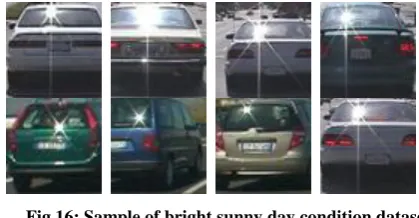
In case 3 that is 6.3 we present the natural condition of bright sunny day with the basic sample of dataset and results.
Fig 16: Sample of bright sunny day condition dataset
Case 3.1 Kernel Type – RBF
Table 5. Classification Summary – Support Vector Machine
Class Name
Total Correct Incorrect Correct (%)
Incorrect (%)
Car 310 301 9 97.09677 2.903226
Non - Car
Histogram of FE (Predictions)
Car Non Car
FE (Predictions) 0
20 40 60 80 100 120 140 160 180 200 220 240 260 280 300 320 340 360
N
o
.
o
f
o
b
se
rva
ti
o
n
s
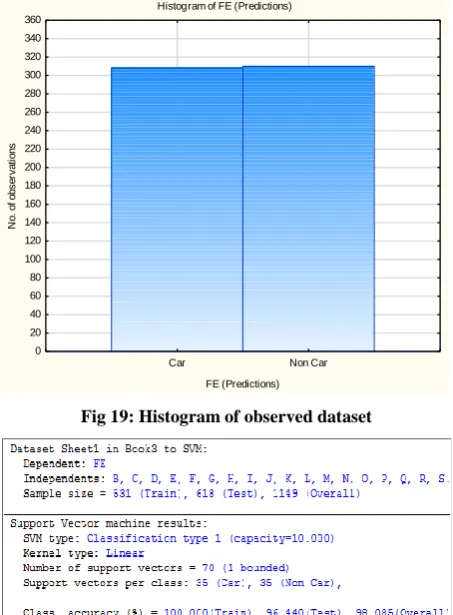
Fig 17: Histogram of observed dataset
Fig 18: Overall performance of detector
Case 3.2 Kernel Type – Linear
Table 6. Classification Summary – Support Vector Machine
Class Name
Total Correct Incorrect Correct (%)
Incorrect (%)
Car 310 298 12 96.12903 3.870968
Non - Car
308 298 10 96.75325 3.246753
Histogram of FE (Predictions)
Car Non Car
FE (Predictions) 0
20 40 60 80 100 120 140 160 180 200 220 240 260 280 300 320 340 360
N
o
.
o
f
o
b
se
rva
ti
o
n
s
Fig 19: Histogram of observed dataset
Fig 20: Overall performance of detector
6.4
Normal Day Light Conditions
In case 4 that is 6.4 we present the natural condition of normal day light with the basic sample of dataset and results.
Fig 21: Sample of normal day light condition dataset
Case 4.1 Kernel Type – RBF
Table 7. Classification Summary – Support Vector Machine
Class Name
Total Correct Incorrect Correct (%)
Incorrect (%)
Car 892 878 14 98.43049 1.569507
Non - Car
Histogram of FE (Predictions)
Car Non Car
FE (Predictions) 0
100 200 300 400 500 600 700 800 900 1000 1100
N
o.
of
ob
s
er
v
at
io
ns
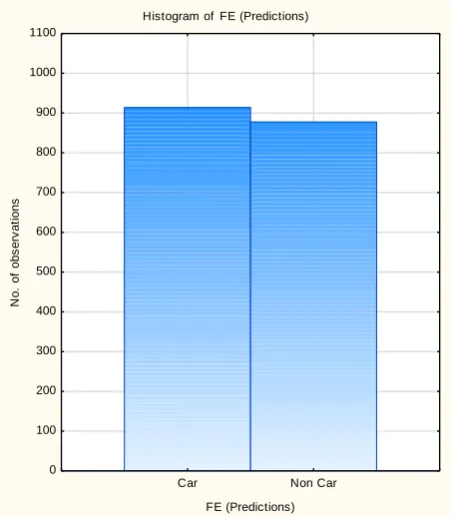
Fig 22: Histogram of observed dataset
Fig 23: Overall performance of detector
Case 4.2 Kernel Type – Linear
Table 8. Classification Summary – Support Vector Machine
Class Name
Total Correct Incorrect Correct (%)
Incorrect (%)
Car 892 858 34 96.18834 3.811659
Non - Car
900 870 30 96.66667 3.333333
Histogram of FE (Predictions)
Car Non Car
FE (Predictions) 0
100 200 300 400 500 600 700 800 900 1000
N
o
.
o
f
o
b
s
e
rv
a
ti
o
n
s
Fig 24: Histogram of observed dataset
Fig 25: Overall performance of detector
6.5
Rainy Conditions
In case 5 that is 6.5 we present the natural condition of rainy day with the basic sample of dataset and results.
Fig 26: Sample of rainy day light condition dataset
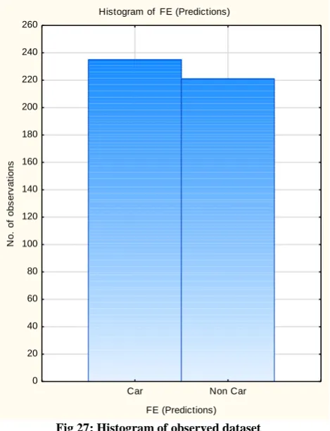
Case 5.1 Kernel Type – RBF
Table 9. Classification Summary – Support Vector Machine
Class Name
Total Correct Incorrect Correct (%)
Incorrect (%)
Car 235 233 2 99.14894 0.851064
Non - Car
Histogram of FE (Predictions)
Car Non Car
FE (Predictions) 0
20 40 60 80 100 120 140 160 180 200 220 240 260
N
o.
of
ob
s
er
v
at
io
ns
Fig 27: Histogram of observed dataset
Fig 28: Overall performance of detector
Case 5.2 Kernel Type – Linear
Table 10. Classification Summary – Support Vector Machine
Class Name
Total Correct Incorrect Correct (%)
Incorrect (%)
Car 235 232 3 98.72340 1.276596
Non - Car
221 219 2 99.09502 0.904977
Histogram of FE (Predictions)
Car Non Car
FE (Predictions) 0
20 40 60 80 100 120 140 160 180 200 220 240 260
N
o
.
o
f
o
b
se
rva
ti
o
n
s
Fig 29: Histogram of observed dataset
Fig 28: Overall performance of detector
7.
CONCLUSION
In this research work, a vehicle detection algorithm based on the gradient and concentrated on shape analysis is used, further our suggested approach for training is based on concatenating the shape feature vector with texture analysis based on Gray level Co-Occurrence matrix. Results show that using gray level co – occurrence matrix feature vector offered a better performance when handling occlusion and different weather and light conditions. Though, occlusion is still challenging also in terms of dataset annotation. In this research, two efficient image features based on texture and shape analysis were implemented and popular classifiers– SVM was studied and their performances for vehicle classification were systematically evaluated under the same experimental setups. For both the shape and texture features, the SVM classifier achieved better performance.
Our experiments demonstrated the superior performance of our detection system by using a both texture and shape analysis. In fact, it was found that employing these method helps to reduce the false detections and improves the detection system’s performance.
Since the suggested system used a monocular camera images for collecting information, further it can be done on a video with a stereo camera.
performance under the scenes of occluded vehicles, as it utilizes Histogram of orientation binning and due to the long length of feature vector it also uses the concept of principal component analysis to filter out the best feature vector from the overall system.
8.
ACKNOWLEDGMENTS
Our thanks to the experts who have contributed towards development of this research work, my teachers, classmates and lab members.
9.
REFERENCES
[1] Adnan Shaout, Dominic Colella, S. Awad, “Advanced Driver Assistance Systems
[2] Past, Present and Future,” Seventh International Computer Engineering Conference (ICENCO), 2011, pp. 321–329.
[3] Andreas Geiger, Philip Lenz and Raquel Urtasun, “Are we ready for Autonomous Driving? The KITTI Vision Benchmark Suite,” IEEE Conference on Computer Vision and Pattern Recognition (CVPR), 2012, pp. 3354 - 3361.
[4] Advance driver assistance systems http://www.freescale.com/webapp/sps/site/overview.jsp? code=ADAS
[5] LG - Safety & Convenience Devices, Advance driver assistance systems
[6] http://www.lgvccompany.com/en/products/adas-camera-systemVision based advance driver assistance
[7] Whei Zhang,Q.M Jonathan Wu,Xiaokang Yang, “Multilevel framework to detect and handle Occlusion,” IEEE Transaction on Intelligent Transport Systems,VOL.9,NO.1,2008
[8] Himanshu Chandel and Sonia Vatta, “Occlusion Detection and Handling: A Review,” International Journal of Computer Applications (0975 – 8887) Volume 120 – No.10, June 2015.
[9] SLAM for dummies
http://ocw.mit.edu/courses/aeronautics-and- astronautics/16-412j-cognitive-robotics-spring-2005/projects/1aslam_blas_repo.pdf.
[10]Herbert Bay, Tinne Tuytelaars, Luc Van Gool ,“SURF: Speeded Up robust features ,”15th International Conference on Pattern Recognition,” 9th European Conference on Computer Vision, Graz, Austria, May 7-13, 2006. Proceedings, Part I , pp. 404-417
[11]P. Felzenszwalb, D. McAllester, D. Ramanan,“ A discriminatively trained, multiscale, deformable part model,” IEEE Conference on Computer Vision and Pattern Recognition, 2008. CVPR 2008. pp. 1 – 8.
[12]Navneet Dalal and Bill Triggs, “Histograms of Oriented Gradients for Human Detection,” IEEE Computer Society Conference on Computer Vision and Pattern Recognition, 2005, pp. 886 - 893 vol. 1.
[13]Ro´merRosales and StanSclaroff, “Improved Tracking of Multiple Humans with Trajectory Prediction and Occlusion Modeling,” IEEE Conf. on Computer Vision and Pattern Recognition,1998
[14]Davi Geiger,Bruce,Ladendorf,Alan Yuille, “Occlusions and Binocular Stereo,”International Journal of Computer Vision,1995
[15]Nello Cristianini and John Shawe-Taylor, “An Introduction to Support Vector Machines and Other Kernel-based Learning Methods”, Cambridge University Press, 2000.
[16]James J. Little and Walter E. Gillet, “Direct Evidence for Occlusion in Stereo and Motion,” Computer Vision — ECCV, 1990