Assessing the application of a laser rangefinder for determining snow depth in inaccessible alpine terrain

www.hydrol-earth-syst-sci.net/14/901/2010/ doi:10.5194/hess-14-901-2010

© Author(s) 2010. CC Attribution 3.0 License.

Earth System

Sciences

Assessing the application of a laser rangefinder for determining

snow depth in inaccessible alpine terrain

J. L. Hood and M. Hayashi

Geoscience University of Calgary, 2500 University Dr., NW, Calgary, AB T2N 1N4, Canada Received: 11 December 2009 – Published in Hydrol. Earth Syst. Sci. Discuss.: 19 January 2010 Revised: 6 May 2010 – Accepted: 21 May 2010 – Published: 4 June 2010

Abstract. Snow is a major contributor to stream flow in alpine watersheds and quantifying snow depth and distribu-tion is important for hydrological research. However, di-rect measurement of snow in rugged alpine terrain is often impossible due to avalanche and rock fall hazard. A laser rangefinder was used to determine the depth of snow in in-accessible areas. Laser rangefinders use ground based light detection and ranging technology but are more cost effec-tive than airborne surveys or terrestrial laser scanning sys-tems and are highly portable. Data were collected within the Opabin watershed in the Canadian Rockies. Surveys were conducted on one accessible slope for validation purposes and two inaccessible talus slopes. Laser distance data was used to generate surface models of slopes when snow cov-ered and snow-free and snow depth distribution was quanti-fied by differencing the two surfaces. The results were com-pared with manually probed snow depths on the accessible slope. The accuracy of the laser rangefinder method as com-pared to probed depths was 0.21 m or 12% of average snow depth. Results from the two inaccessible talus slopes showed regions near the top of the slopes with 6–9 m of snow accu-mulation. These deep snow accumulation zones result from re-distribution of snow by avalanches and are hydrologically significant as they persist until late summer.

Correspondence to: J. L. Hood ([email protected])

1 Introduction

Snow is a major component of the annual water balance in alpine watersheds (Kattelmann and Elder, 1991), and snow depth and distribution measurements are important to hydro-logical research (Flerchinger et al., 1992). However, direct measurement of snow is time consuming, and in many alpine areas, often impractical or impossible due to steep slopes with rock fall and avalanche hazard. In high elevation moun-tain regions, snowmelt influences the timing and quantity of water delivered to rivers and streams. Hydrological process studies in alpine headwaters are important for understanding what changes may occur within a changed climatic regime (Zierl and Bugmann, 2005). Accurate quantification of the hydrological inputs (rain, snowmelt, glacier melt) and snow-pack parameters in alpine watersheds are needed for process-based studies to understand hydrologic responses of alpine watersheds to the inputs. Accurately quantifying snow depth and distribution is also important for validation of snowmelt energy balance models (Cline et al., 1998) and snow distri-bution models (Liston and Elder, 2006), as well as for appli-cations in avalanche research (Prokop, 2008).

in small watersheds. Additionally, in alpine watersheds, avalanche and rock fall hazard limits which areas can be sur-veyed safely. As a result of the above limitations, extensive resources (Dozier and Painter, 2004) have been directed to-wards remote methods of determining snow pack properties such as snow covered area (SCA), snow depth, density and snow water equivalent (SWE). A method that is able to deter-mine all of these properties simultaneously does not yet exist. Satellite imagery can be useful in delineating SCA at high spatial and temporal resolution (Dozier and Painter, 2004; Rosenthal and Dozier, 1996). It is, however, limited by diffi-culties in data capture due to frequently cloudy conditions in mountain regions and does not provide information regarding snow volume. The light detection and ranging (LiDAR) data can be used to determine snow depth (Hopkinson et al., 2001) from the difference in elevation between snow-covered sur-faces and snow-free sursur-faces. LiDAR data have recently been used for investigating spatial snow distribution in Colorado (Trujillo et al., 2007; Fassnacht and Deems, 2006; Deems et al., 2006; Trujillo et al., 2009) although, at present, acqui-sition of LiDAR data is very expensive and requires special expertise. Passive microwave sensors mounted on satellites show promise for determining SWE and these methods con-tinue to improve (Foster et al., 2005); however, the spatial resolution remains too coarse for studies in small watersheds and is limited by underestimation of SWE in alpine regions (Foster et al., 2005).

Terrestrial laser scanning (TLS) is a ground-based LiDAR technique that is capable of producing high spatial resolution scans of the surface and has been used in numerous applica-tions including determining snow depth in alpine terrain for use in avalanche research (Prokop, 2008; Prokop et al., 2008; Schaffhauser et al., 2008). TLS produces a high density (hor-izontal spacing of 3–6 cm) point cloud and the capability to measure changes in snow depth to within 10 cm (Prokop, 2008; Prokop et al., 2008). However, TLS units are at present quite expensive and outside of the domain of many research budgets. Laser rangefinder distance devices are based on similar laser technology as TLS, but rely on manual point data retrieval instead of scanning. A laser rangefinder re-quires that the operator sights and shoots at each target point; whereas, a scanning unit can be automated to collect point data over a specified region. Laser rangefinders can be pur-chased for a fraction of the price of TLS units and for small scale applications they present a viable alternative for deter-mining distances to inaccessible areas. Laser rangefinders have been used previously in diverse research applications such as structural bedrock mapping of the Sheep Mountain anticline (Allwardt et al., 2007), mapping of ground fissures involved in coal bed fires (Ide et al., 2010) and recording po-sitions of rutting elk and their behaviour with regards to ve-hicle traffic (St. Clair and Forrest, 2009). A laser rangefinder has also been used to create small scale digital terrain models by interpolating point measurements (Lewicki et al., 2007). To our knowledge, use of a laser rangefinder for determining

distributed snow depth is a unique application of this tech-nique. The laser model used in this study was a Lasercraft Contour XLRic which can be purchased for under US$6 000. In comparison, the typical price range for a TLS system is US$100 000–$250 000. A laser rangefinder system has the advantage of being very portable with all of the necessary equipment easily transported by a single person and is a po-tentially viable alternative to TLS for measuring snow depth. In this study we attempt to use a laser rangefinder distance device to assess the depth of snow in dangerous to access areas within the Opabin watershed in the Canadian Rock-ies (see site description below). Approximately 58% of the watershed is inaccessible because of extremely rugged ter-rain. Slope angles in the inaccessible region are dominantly greater than 50 degrees and accumulated snow is transported to lower elevations via spindrift and small slough avalanches. The snow in these preferential accumulation zones is an im-portant component of the annual snowpack and often per-sists through to the end of the summer months. These zones comprise 8% of the watershed but are typically inaccessible for manual snow measurements due to exposure to rock fall and avalanche hazard. Therefore, the objectives of this study were to: (1) assess the applicability of a laser distance device for determining maximum snow accumulation and (2) assess the hydrological significance of increased snow accumula-tion at the base of steep cliff walls from spindrift and slough avalanching.

2 Methods

2.1 Overview of laser rangefinder method

A bi-pod mounted laser rangefinder (Lasercraft Contour XL-Ric) (Table 1) was used to generate a dataset of surface el-evations of snow-covered surfaces. The laser rangefinder is based on LiDAR technology where an infrared laser signal is transmitted and returned from a surface. The time delay between transmission and receipt of the signal is used to de-termine the distance to the target based on the speed of light (Lasercraft, 2007). In addition to distance, point data col-lected with the laser provide measurement offsets from the laser position which include inclination and azimuth. If the precise location of the laser is known, the horizontal coordi-nates and elevation can be determined using simple geomet-ric calculations. The point elevation data is then interpolated to generate a digital elevation surface and surfaces generated from subsequent surveys are differenced to obtain the change in elevation.

2.2 Laser specifications

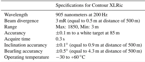
Table 1. Laser specifications.

Specifications for Contour XLRic Wavelength 905 nanometers at 200 Hz

Beam divergence 3 mR (equal to 0.5 m at distance of 500 m) Range Max: 1850, Min: 3 m

Accurancy ±0.1 m to a white target at 85 m Acquire time 0.3 s

Inclination accurancy ±0.1◦(equal to 0.9 m at distance of 500 m) Bearling accurancy ±0.5◦(equal to 4.3 m at distance of 500 m) Operating temperature −30 to +60◦C

surveying from safe locations. It is worth noting, that maxi-mum range is obtained at night and during cloudy conditions; whereas, the maximum range to a white target during bright daylight is 800 m (Lasercraft, 2007). Positional uncertainty becomes an issue at large distances because of limitations in the laser rangefinder accuracy. The manufacturer stated in-clination accuracy (±0.1◦) and bearing accuracy (±0.5◦), re-sults in up to 0.9 m of uncertainty in the vertical position and 4.3 m in the horizontal position of each laser point, respec-tively, at a range of 500 m. Additionally, the beam divergence angle (the increase in the size of the beam with distance) also limits the accuracy at full range (Table 1). A maximum range of 500 m was used in this study. A common concern with laser surveying is transmission of the beam into the snow sur-face. A study using TLS (laser wavelength of 900 nm) found that transmission into snow as compared to a snow surface covered by a foil blanket was negligible (Prokop, 2008). 2.3 Comparison of laser rangefinder and TLS

The laser rangefinder has similarities and differences from a TLS system that make it both more and less suitable for this application. Both methods involve creating a digital terrain surface by interpolating point measurements; however, the TLS method generates a higher resolution dataset (Prokop, 2008) which enables smaller features to be resolved. In con-trast, interpolating lower spatial resolution point data from a laser rangefinder (Table 2) results in a more generalized sur-face and introduces greater uncertainty from the interpolation method. TLS models typically have a beam divergence of 0.25–1.3 mrad (Prokop, 2008) depending on the system. This is much smaller than a laser rangefinder (Table 1) which fur-ther aids in resolution of small scale features. Both systems require adequate signal return to determine the distance to the surface and are impacted by conditions such as fog and lower signal return from wet snow surfaces (Prokop, 2008); how-ever, the quality of laser rangefinder signal return is assessed in-situ because the instrument is manually operated. A laser rangefinder is significantly more portable (1.6 kg) than TLS systems (10–18 kg) (Ingesand, 2006) making it more suit-able for conducting surveys in areas with poor access. The

Slope (degrees) 0 - 10

10- 20

20- 30

30 - 40

40 - 50

50 - 60

60 - 70

70 - 80

80 - 90

0

´

! .

Legend

!

. Weather Station

a b

c

1 2

3

Laser survey

Laser survey Not accessible Opabin Glacier

0

´

B.

location

Fig. 1. (A) Opabin watershed map with locations of laser surveys (1-lower talus, 2-validation slope, 3-upper talus), laser position (a-lower talus, b-validation slope, c-upper talus) and inaccessible area. Contour interval 25 m. (B) Opabin watershed slope map.

portability and ease of set-up also allow for multiple surveys in a single day. TLS systems are more appropriate when high resolution data is required and cost and portability are of no concern. However, a laser rangefinder provides a viable al-ternative for determining snow depth at a much lower cost, with better portability.

2.4 Study site

This research was conducted in the Opabin watershed within the Lake O’Hara Research Basin (51.35◦_{N, 116.32}◦_E)

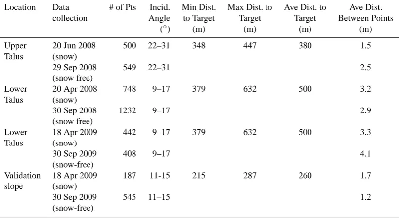
Table 2. Laser data collection date, number of points, incidence angle, distance to target and distance between points for four laser surveys.

Location Data # of Pts Incid. Min Dist. Max Dist. to Ave Dist. to Ave Dist.

collection Angle to Target Target Target Between Points

(◦) (m) (m) (m) (m)

Upper 20 Jun 2008 500 22–31 348 447 380 1.5

Talus (snow)

29 Sep 2008 549 22–31 2.5

(snow free)

Lower 20 Apr 2008 748 9–17 379 632 500 3.2

Talus (snow)

30 Sep 2008 1232 9–17 2.9

(snow free)

Lower 18 Apr 2009 442 9–17 379 632 500 3.3

Talus (snow)

30 Sep 2009 408 9–17 4.1

(snow-free)

Validation 18 Apr 2009 187 11-15 215 287 260 1.7

slope (snow)

30 Sep 2009 545 11–15 1.2

(snow-free)

many zones of near vertical cliff walls. An automatic weather station (Fig. 1) was installed in August 2004 to measure tem-perature, humidity, wind speed and direction, precipitation, snow depth, and radiation. The watershed has an annual average precipitation of 1000–1200 mm, average snow pack of 575–700 mm water equivalent (assessed from April snow surveys at peak accumulation) and is snow-covered from November through to June or July. The geology of the water-shed consists of quartzite and sandstone at lower elevations (valley bottom) with dominantly carbonates at upper eleva-tions (mountain peaks) (Lickorish and Simony, 1995).

The steep cirque walls results in transport of snow from higher elevations to lower elevations through the contin-ual process of slough avalanches. The cirque walls are too steep to accumulate significant amounts of snow; therefore, mass movement of snow (i.e. large point release or slab avalanches) only occurs in a few localized areas. The cliff walls are also prone to significant rock fall as a result of the friable carbonate geology at upper elevations and multiple small fault zones. The combination of snow transport and rock fall potential makes it extremely hazardous to deploy field teams for manual measurement of snow depth and den-sity in a portion of the watershed; however, these areas are zones of preferential accumulation.

2.5 Data collection and analysis methods

Two areas (“upper talus” slope and “lower talus” slope) were selected for this analysis in order quantify snow accumula-tion at the base of cliff walls (Fig. 1). In a third locaaccumula-tion (“val-idation slope”) both laser data and manually measured snow depth data were collected for the purpose of validating laser

results. The lower talus slope was surveyed at peak snow accumulation (mid April) in 2008 and 2009, the upper talus slope was surveyed in June 2008 and the validation slope was surveyed at peak snow accumulation in 2000. The validation slope is located in the interior of the watershed and is not exposed to snow accumulation via avalanches. The upper and lower talus slopes are both overshadowed by cliff walls with average slopes of 65–70◦_{and approximately 420 m of}

The laser was set-up at a stable platform using a bi-pod and the location was recorded using differential GPS (Sokkia GSR2700 ISX) which is accurate to 10 mm horizontally and 20 mm vertically. The location was marked with a steel pin for re-locating the laser for the snow-free survey; addition-ally, the coordinates were recorded with the differential GPS during both surveys. A deep snowpack (ca. 2 m) at the laser location necessitates that the laser is set up at the snow sur-face; therefore snow depth at the laser location is measured to aid in re-locating the laser for the snow-free survey. The snow surface was compacted on foot prior to the laser set up and the distance between the laser and the ground was mea-sured prior to and following the survey (with a depth probe) to ensure that the set up did not settle into the snow. Accurate elevation data at the laser location is important to the success of the method, as all laser offsets are converted to Universal Transverse Mercator (UTM) coordinates and elevation rela-tive to the laser location. The re-location of the laser was precise to within 3–8 cm horizontally and 12–17 cm verti-cally. The discrepancy in the vertical position of the laser results is a result of positioning the laser over snow during the spring survey.

At each location 187–1232 points were measured with a horizontal spacing of 1.5–4.1 m (Table 2). The distance to the slope varied between 260–500 m. The distance to vali-dation slope was slightly less than the other slopes (average distance of 260 m, versus 380–500 m) as was necessary to achieve similar viewing and incidence angles. The laser po-sition was, in all cases, lower than the target slopes. Laser in-cidence angles ranged from 9–31◦(with 0◦representing par-allel to the slope and 90◦_{perpendicular to the slope). The}

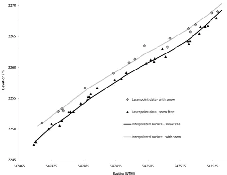
in-cidence angles at the validation slope were in a similar range as the lower talus slope (Table 2). The upper talus slope had greater incidence angles. Greater incidence angles result in greater accuracy (Ingesand, 2006); however, incidence an-gles could not be increased without exceeding the range of the laser (for daylight) given the geometry of the watershed. Digital elevation surfaces were generated using the ESRI ArcGIS spatial computing software. Snow and snow-free digital elevation surfaces were created by spatially in-terpolating point data using a local polynomial interpolator. This type of interpolator is inexact which smoothes the data and results in a generalized surface (Fig. 2). Smoothing is necessary because of the vertical uncertainty associated with each point measurement (see discussion above). Therefore, an exact interpolator such as kriging would result in abrupt changes in the surface. The resolution of the interpolated surfaces was 0.2 m. The elevation of the interpolated snow-free surface (raster data) was then subtracted from that of the interpolated snow-free (i.e. ground) surface to obtain an esti-mate of snow depth at the time of the initial survey.

2270

2265

2260

(m)

2255

Elevation

(

Laser pointp  data ‐with snow

Laser point data ‐snow free

Interpolated surface ‐snow free 2250

Interpolated surface ‐with snow

2245

547465 547475 547485 547495 547505 547515 547525

Easting (UTM)

Fig. 2. Measured laser point data and local polynomial interpola-tion.

2.6 Validation methods

Manual snow depth measurements were made at the vali-dation slope on the same day as the laser survey. Snow depth data were collected using a centimetre graduated depth probe. Snow depth was measured at four points within a square metre to minimize the influence of local topographic variability and these values were subsequently averaged to obtain the snow depth at that point. Average of the stan-dard deviation of four depth points was 0.13 m. A Trimble GeoXH GPS was used to record the mid-point location of the manual snow depth measurement and these points were differentially post-corrected using data from a base station in Calgary (160 km east of the site). Ten data points had GPS positions with greater than one metre of horizontal error and were discarded. The manual snow depth measurement was compared to the snow depth determined by the laser analyses (hereafter referred to as “laser snow depth”) by extracting the raster value of the interpolated snow depth surface that corre-sponded with the manual point measurement using ArcGIS software.

3 Results

3.1 Comparison of measured and laser-derived snow depths at the validation site

Elev

ation (m)

Northing Easting

A. B.

C. D.

Elev

ation (m)

Northing Easting

Snow Depth (m)

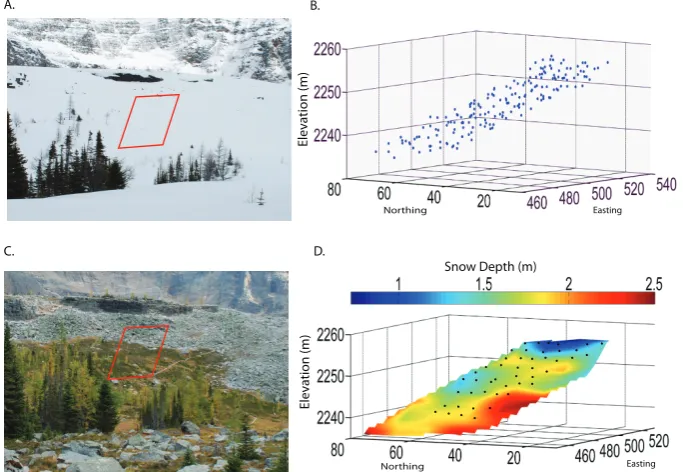
Fig. 3. Validation slope (A) snow covered (18 April 2009), (B) distribution of laser points (April), (C) snow free (30 September 2009), (D) laser snow depth (black dots show locations of manual snow depth measurements).

1 1.5 2 2.5

Snow

Depth

(m)

0 0.5

0 5 10 15 20 25 30 35 40 45

Data Point

Laser snow depth

Measured snow depth

Fig. 4. Manually measured versus calculated snow depths at the validation slope. Error bars represent the range of measured depths at each point.

data (Fig. 3d). The center position of each of the 44 manual measurement locations was used to extract the correspond-ing laser snow depth from the interpolated snow depth raster (Fig. 3d). In Fig. 3, the measured snow depth at each of the measurement locations is compared to laser snow depth at the same location. The location number in Fig. 3 starts from upper left of the survey area (see Fig. 3d) and sequen-tially increases from the top to bottom, and left to right. The error bars represent the range in measured snow depth as determined by four measurements. Manually measured and

2.4 2.6

1 8 2 2.2

m

)

1.4 1.6 1.8

n

ow

depth

(m

y = 0.873x + 0.2303 1

1.2

M

easur

e

d

sn

R² = 0.6688

0.4 0.6 0.8

M

0 0.2

0 0 2 0 4 0 6 0 8 1 1 2 1 4 1 6 1 8 2 2 2 2 4 2 6

0 0.2 0.4 0.6 0.8 1 1.2 1.4 1.6 1.8 2 2.2 2.4 2.6

Laser Snow Depth (m)

Fig. 5. Scatter plot of manually measured versus laser snow depth at the validation slope. Error bars show the variation in measured snow depth.

Table 3. Measured versus modeled mean, minimum, and maximum snow depth and standard deviation.

Mean Snow Depth (m) Minimum (m) Maximum (m) Standard Deviation

Measured 1.71 0.73 2.43 0.40

Calculated 1.70 0.79 2.45 0.37

Elev

ation (m)

Northing Easting

A. B.

C. D.

Elev

ation (m)

Northing _Easting

Snow Depth (m)

Fig. 6. Upper talus slope (A) snow covered (20 June 2008), (B) distribution of laser points (June), (C) snow free (29 September 2008), (D) laser snow depth.

of the scatter in Fig. 5 may be attributed to uncertainty in-herent in using a polynomial interpolation. There is addi-tional uncertainty in the measured snow depth as it is impos-sible to quantify the true value of a continuously distributed medium with point measurements. The horizontal accuracy of the GPS used for locating manual snow depth points was 0.5–0.9 m which may introduce additional uncertainty. How-ever, despite the uncertainty associated with the snow depth at a given point, the trends of high and low snow depths (Fig. 4) and the mean snow depths clearly indicate that the average snow depth distribution is well characterized. The average measured snow depth (Table 3) was 1.71 m and the laser snow depth average was 1.70 m. Likewise, the mea-sured (laser snow depth) minimum of 0.73 m (0.79 m) and maximum of 2.43 m (2.45 m) indicate that the overall trend and features of the snow depth distribution are well captured using a laser distance device. The average point spacing at the validation slope is less than at the talus slopes (Table 2). The analysis on the validation slope was repeated using only 25% of the points to determine the sensitivity of the method to point spacing. The mean snow depth was unchanged, in-dicating this method is insensitive to the point spacing.

The snow depth distribution map (Fig. 3d) shows a large range in accumulated snow depths. Shallow snow on the west side (upper portion of the slope) is likely the result of a small cliff (approximately 5 m high) that shelters the slope immediately below (Fig. 3a and d) which is also indicated by exposed rocks at the base of the cliff. The remaining depth variation results from depressions in the surface topography (as determined from the snow-free laser data set) which pref-erentially accumulate snow.

3.2 Talus slope snow accumulation patterns

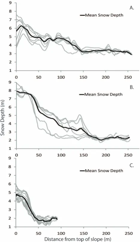
There is a large range in snow depths on the talus slopes with much greater accumulation at the top of the slope versus the bottom (Figs. 6d, 7e and f). The upper talus slope has re-maining snow accumulation in June of 1.15 m at the base of the slope and nearly 6 m at the top of the slope (Fig. 6d). The range in snow depths at the lower talus slope at the peak of the accumulation was 2.8–7.6 m in 2008 and 1.7–8.9 m in 2009 (Fig. 7e and f).

A. B.

C. D.

Easting

Northing _Northing

Easting Easting Northing

Easting Northing

Snow Depth (m) F. Snow Depth (m) E.

Fig. 7. Lower talus slope (A) snow covered (28 April 2009), (B) snow-free (30 September 2009), (C) distribution of laser points

(20 April 2008), (D) distribution of laser points (18 April 2009), (E) laser snow depth (2008), (F) laser snow depth (2009).

at the top of the slope to shallow snow at the bottom of the slope whereas in 2009 there is additional cross – slope vari-ation. This may be the result of a greater amount of snow redistribution by wind in 2009 than in 2008. In the winter of 2009 a greater proportion of high-wind events were from the southeast whereas the preceding three years of record indi-cate a dominant southwest winter flow regime. This change in wind direction would result in greater accumulation on the lee side of the slope which is indicated in the lower talus slope accumulation profile for 2009. In addition to the change in wind direction, average wind speeds were higher during 2009.

3.3 Contribution of slough avalanches to snow accumulation and hydrological importance

slough avalanche paths which may be a possible explanation for the larger zone of influence at this site. Additionally, the cliffs at the lower cliff site have a tendency for cornice devel-opment that is not present at the upper talus site.

The snow deposited through the process of slough avalanching is an important component of the annual water balance and these deposits often persist into the late summer (Fig. 7b) due to the depth of the deposits and their position on shaded northeast facing slopes. Avalanche accumulation zones comprise 8% of the watershed area. Mean snow depth at the lower talus site in 2008 and 2009 was 4.1 m. Assuming that this snow depth is representative of avalanche accumu-lation zones throughout the watershed, and assuming a mean snow density of 450 kg m−3(derived from depth-density re-gression equations in the watershed), the water stored as snow in these deposits is equivalent to 16% of the annual stream flow, and 54% of the stream flow from 1 August to 30 September. Therefore, it is quite likely that these de-posits play an important role in prolonging the snowmelt sea-son. Further work is in progress to characterize this contri-bution using a distributed snow melt model in conjunction with characterization of snow-covered-area using oblique-angle photographs (Corripio, 2004).

The different patterns of snow accumulation at the two talus sites are an important indication of the variability that may be expected throughout the watershed. This study has provided insight into the importance of avalanche snow transport on the alpine water balance. However, it must be emphasized that snow accumulation via these mechanisms may vary considerably throughout the watershed. Quan-tifying the zone of influence of the spindrift and slough avalanches will be useful in determining snow water equiva-lent in the watershed.

4 Conclusions

A laser rangefinder distance device was used to quantify snow depth on talus slopes in an alpine watershed. The de-vice was used to determine distance to snow-covered slopes in the spring and again in the fall during snow-free con-ditions. The point data were then used to generate digital surface models of the snow covered and snow-free surfaces which can be used to determine snow depth by differenc-ing of the two surfaces. On the validation slope, the av-erage of laser-derived snow depth (1.70 m) was essentially identical to that of manually measured snow depth (1.71 m), while the comparison of individual grid cells had a root-mean-squared error of 0.21 m or 12% of the average snow depth. Therefore, the laser method offers unbiased estimates of snow depth on slopes that are not accessible for manual snow survey and captures the spatial pattern of snow depth distribution with reasonable accuracy. Terrestrial laser scan-ners have been used in similar applications and produce data with higher spatial resolution (Prokop, 2008; Prokop et al.,

Fig. 8. Profiles of snow depth accumulation (A) lower talus, 2008, (B) lower talus, 2009, (C) upper talus, 2008. Grey lines are ex-tracted snow depth profiles. Black lines are the mean snow depths of the extracted snow depth profiles.

2008); however, a laser rangefinder presents a more cost ef-fective and portable means of measuring average snow depth in deep snow.

Snow depth distribution obtained using the laser rangefinder method showed very deep snow accumulation at the top of talus slopes in the watershed as a result of slough avalanching from the steep cirque walls overhead. The amount of snow stored in these deep snow zones (ca. 6– 9 m) is equivalent to 16% of average annual stream flow, and the snow persists into late August, possibly extending the snowmelt season.

method of measuring snow depth in complex alpine areas and contributes to an increased understanding of the hydro-logic impact of snow redistribution by avalanches.

Acknowledgements. The authors are grateful for field assis-tance from Jackie Randall, Greg Langston, Nathan Green and Danika Muir. Logistical support was provided by Lake O’Hara

Lodge and Parks Canada. Funding was provided by Alberta

Ingenuity, G8 Legacy Chair in Wildlife Ecology, Natural Sciences and Engineering Research Council, the Canadian Foundation for Climate and Atmospheric Sciences (IP3 Network), and Environ-ment Canada Science Horizons Program. Lastly, we would like to thank the two anonymous reviewers whose feedback greatly improved this manuscript.

Edited by: S. Carey

References

Allwardt, P. F., Bellahsen, N., and Pollard, D. D.: Curvature and fracturing based on global positioning system data collected at sheep mountain anticline, Wyoming, Geosphere, 3, 408–421, 2007.

Cline, D. W., Bales, R. C., and Dozier, J.: Estimating the spatial distribution of snow in mountain basins using remote sensing and energy balance modeling, Water Resour. Res., 34, 1275–1285, 1998.

Corripio, J. G.: Snow surface albedo estimation using terrestrial photography, Int. J. Remote Sens., 25, 5705–5729, 2004. Deems, J. S., Fassnacht, S. R., and Elder, K. J.: Fractal distribution

of snow depth from lidar data, J. Hydrometeorol., 7, 285–297, 2006.

Derksen, C., Brown, R., Walker, A., and Brasnett, B.: Compari-son of model, snow course, and passive microwave derived snow water equivalent data for Western North America, 59th Eastern Snow Conference: Stowe, Vermont, 203–213, 2002.

Dozier, J. and Painter, T. H.: Multispectral and hyperspectral remote sensing of alpine snow properties, Annu. Rev. Earth Pl. Sc., 32, 465–494, 2004.

Dressler, K. A., Fassnacht, S. R., and Bales, R.: A comparison of snow telemetry and snow course measurements in the Colorado River basin, J. Hydrometeorol., 7, 705–712, 2006.

Elder, K., Dozier, J., and Michaelsen, J.: Snow accumulation and distribution in an alpine watershed, Water Resour. Res., 27, 1541–1552, 1991.

Fassnacht, S. and Deems, J. S.: Measurement sampling and scaling for deep montane snow depth data, Hydrol. Process., 20, 829– 838, 2006.

Flerchinger, G., Cooley, K., and Ralston, D.: Groundwater response to snowmelt in a mountainous watershed, J. Hydrol., 133, 293– 311, 1992.

Foster, J. L., Sun, C., Walker, J. P., Kelly, R., Chang, A., Dong, J., and Powell, H.: Quantifying the uncertainty in passive mi-crowave snow water equivalent observations, Remote Sens. En-viron., 94, 187–203, 2005.

Hopkinson, C., Demuth, M. N., Sitar, M., and Chasmer, L. E.: Map-ping the spatial distribution of snowpack depth beneath a variable forest canopy using airborne laser altimetry, 58th Eastern Snow Conference, Ottawa, Ontario, Canada, 249–253, 2001.

Ide, T. S., Pollard, D. D., and Orr Jr., F. M.: Fissure formation and subsurface subsidence in a coalbed fire, Int. J. Rock Mech. Min., 47, 81–92, 2010.

Ingesand, H.: Metrological aspects in terrestrial laser-scanning technology, in: Proceedings of the 3rd International Association of Geology/12th International Federation of Surveyors Sympo-sium, Baden, Austria. 2006

Kattelmann, R. and Elder, K.: Hydrologic characteristics and water balance of an alpine basin in the Sierra Nevada, Water Resour. Res., 37(7), 1553–1562, 1991.

Kˇremen, T., Koska, B., and Posp´ıˇsil, J.: Verification of laser scan-ning systems quality, in: Proceedings 23rd International Federa-tion of Surveyors Congress, Munich, Germany, 2006.

Lasercraft: Contour XLRic Operator’s Manual, LaserCraft Inc., Norcross, GA, 2007.

Lewicki, J. L., Hilley, G. E., Tosha, T., Aoyagi, R., Ya-mamoto, K., and Benson, S. M.: Dynamic coupling of

vol-canic Co2flow and wind at the Horseshoe Lake tree kill,

Mam-moth mountain, California, Geophys. Res. Lett., 34, L03401, doi:10.1029/2006GL028848, 2007.

Lickorish, W. H. and Simony, P. S.: Evidence for late rifting of the Cordilleran margin outlined by stratigraphic division of the Lower Cambrian Gog group, Rocky Mountain main ranges, British Columbia and Alberta, Can. J. Earth Sci., 32, 860–874, 1995.

Liston, G. E. and Elder, K.: A distributed snow-evolution modeling system (Snowmodel), J. Hydrometeorol., 7, 1259–1276, 2006. Pomeroy, J., Essery, R., and Toth, B.: Implications of spatial

dis-tributions of snow mass and melt rate for snow-cover depletion: Observations in a subarctic mountain catchment, Ann. Glaciol., 38, 195–201, 2004.

Prokop, A.: Assessing the applicability of terrestrial laser scanning for spatial snow depth measurements, Cold Reg. Sci. Technol., 54, 155–163, 2008.

Prokop, A., Schirmer, M., Rub, M., Lehning, M., and Stocker, M.: A comparison of measurement methods: Terrestrial laser scanning, tachymetry and snow probing for the determination of the spatial snow-depth distribution on slopes, Ann. Glaciol., 49, 210–216, 2008.

Rosenthal, W. and Dozier, J.: Automated mapping of montane snow cover at subpixel resolution from the Landsat thematic mapper, Water Resour. Res., 32, 115–130, 1996.

Schaffhauser, A., Adams, M., Fromm, R., Jorg, P., Luzi, G., Noferini, L., and Sailer, R.: Remote sensing based retrieval of snow cover properties, Cold Reg. Sci. Technol., 54, 164–165, 2008.

St. Clair, C. C. and Forrest, A.: Impacts of vehicle traffic on the dis-tribution and behaviour of rutting elk, Cervus elaphus, Behavior, 146, 393–413, 2009.

Trujillo, E., Ramirez, J. A., and Elder, K. J.: Topographic, meteo-rologic, and canopy controls on the scaling characteristics of the spatial distribution of snow depth fields, Water Resour. Res., 43, 1575–1590, 2007.

Trujillo, E., Ramirez, J. A., and Elder, K. J.: Scaling properties and spatial organization of snow depth fields in sub-alpine forest and alpine tundra, Hydrol. Process., 23, 1575–1590, 2009.