http://www.sciencepublishinggroup.com/j/ijtam doi: 10.11648/j.ijtam.20170306.19
ISSN: 2575-5072 (Print); ISSN: 2575-5080 (Online)
A Hybrid Genetic Algorithm-Simulated Annealing for
Integrated Production-Distribution Scheduling in Supply
Chain Management
Setareh Abedinzadeh
1, Hamid Reza Erfanian
2, *, Mojtaba Arabmomeni
31
Department of Industrial Engineering, University of Science and Culture, Tehran, Iran 2Department of Mathematics, University of Science and Culture, Tehran, Iran
3Department of Industrial Engineering, University of Science and Technology, Tehran, Iran
Email address:
[email protected] (H. R. Erfanian) *Corresponding author
To cite this article:
Setareh Abedinzadeh, Hamid Reza Erfanian, Mojtaba Arabmomeni. A Hybrid Genetic Algorithm-Simulated Annealing for Integrated Production-Distribution Scheduling in Supply Chain Management. International Journal of Theoretical and Applied Mathematics.
Vol. 3, No. 6, 2017, pp. 229-238. doi: 10.11648/j.ijtam.20170306.19
Received: September 27, 2016; Accepted: January 10, 2017; Published: January 14, 2018
Abstract:
In this paper, we present an integrated production-distribution (P-D) model which considers rail transportation to move deteriorating items. The problem is formulated as a mixed integer programming (MIP) model, which could then be solved using GAMS optimization software. A hybrid genetic algorithm-simulated annealing (GA-SA) is developed to solve the real-size problems in a reasonable time period. The solutions obtained by GAMS are compared with those obtained from the hybrid GA-SA and the results show that the hybrid GA-SA is efficient in terms of computational time and the quality of the solution obtained.Keywords:
Integrated Production-Distribution Planning, Rail Transportation, Deteriorating Items, Scheduling, Hybrid Genetic Algorithm-Simulated Annealing1. Introduction
A supply chain (SC) may be considered as an integrated process in which a group of several organizations, such as suppliers, producers, distributors and retailers, work together to acquire raw materials with a view to converting them into end products which they distribute to retailers [1]. The two core optimization problems in a SC are production and distribution planning. In the production planning, decisions such as hiring and firing of labors, regular time and overtime production, subcontracting and machine capacity levels are made for a definite planning horizon (i.e. usually a one year period). Whereas, in the distribution planning decisions relates to determining which facility (ies) would supply demands of which market(s) [2].
Unlike traditional supply chains with members competing to reduce their individual costs, the overall cost of the entire supply chain is minimized in a cooperative
supply chain. The savings from cooperation may be shared among the members, while a lower average cost and a lower cost variation is materialized for individual members.
proposed approach yields high-quality solutions within reasonable computation times. Pasandideh et al, considered a bi-objective optimization of a multi-product multi-period three-echelon supply-chain-network problem [13]. The network consists of manufacturing plants, distribution centers (DCs), and customer nodes. The majority of the parameters in this network including fixed and variable costs, customer demand, available production time, set-up and production times, all are considered stochastic. The goal is to determine the quantities of the products produced by the manufacturing plants in different periods, the number and locations of the warehouses, the quantities of products transported between the supply chain entities, the inventory of products in warehouses and plants, and the shortage of products in periods such that both the expected and the variance of the total cost are minimized. The problem is first formulated into the framework of a single-objective stochastic mixed integer linear programming model. Then, it is reformulated into a bi-objective deterministic mixed integer nonlinear programming model. To solve the complicated problem, a non-dominated sorting genetic algorithm (NSGA-II) is utilized next. As there is no benchmark available in the literature, another GA-based algorithm called non-dominated ranking genetic algorithm (NRGA) is used to validate the results obtained. Some numerical illustrations are provided to show the applicability of the proposed methodology and select the best method using a t-test along with the simple additive weighting (SAW) method. Priyan et al, considered a distributor and a warehouse consisting of a serviceable part and a recoverable part supply chain problem in which there are several products, the distributor has limited space capacity and budget to purchase all products [14]. A mathematical model is employed to optimize the order quantity, lead time and total number of deliveries with the objective of minimizing system total cost. A simple Lagrangian multiplier technique to solve the model which is a constrained non-linear programming. At the end, numerical and sensitivity analysis are given to show the applicability of the proposed model in real-world product returns inventory problems.
In addition, rail transportation has been widely used in supply chain management (SCM). Yaghini et al, presented a comprehensive review of multi-commodity network design (MCND) problems modeling, their applications in rail freight transportation planning, and solution methods which have been developed to solve them [16]. Hajiaghaei-Keshteli et al, proposed an integrated production and transportation model, which considers rail transportation to deliver orders from a facility to the customers [5]. The problem is to determine both production schedule and rail transportation allocation of orders to optimize customer service at minimum total cost. Different destinations of the trains, trains' capacities, and different transportation costs are the main aspects of the work which are considered. A heuristic, two meta-heuristics and some related procedures are developed to cope with the NP-hardness of the problem. Besides, Taguchi experimental
design method is utilized to set and estimate the proper values of the algorithms' parameters to improve their performance. For the purpose of performance evaluation of the proposed algorithms, various problem sizes are employed and the computational results of the algorithms are compared with each other. Besides, Hajiaghaei-Keshteli et al, developed the integrated scheduling of production and rail transportation. The problem is to determine both production schedule and rail transportation allocation of orders to optimize customer service at minimum total cost [6]. Some procedures and heuristics are utilized to encode the model in order to address it by two capable meta-heuristics: GA, and Keshtel algorithm (KA). Taguchi experimental design method is utilized to set and estimate the proper values of the algorithms’ parameters to improve their performance. Besides, various problem sizes are employed and the computational results of the algorithms are compared with each other.
Over the past few days, there have been fruitful efforts for considering deteriorating items in SCM. Ghiami et al, regarded a single-manufacturer, multi-buyer model for a deteriorating item with finite production rate [3]. The authors relaxed the assumption on the production capacity and found the average inventory of the supplier. It is shown that in case the production rate is not high, the existing models may not be sufficiently accurate. Also a sensitivity analysis is conducted to show how the model reacts to changes in parameters. Maihami et al, considered the problem of replenishment policy and pricing for non-instantaneous deteriorating items subject to promotional effort [12]. A price dependent stochastic demand function in which shortages are allowed and partially backlogged, is adopted. The major objective is to simultaneously determine the optimal selling price, the optimal replenishment schedule, and the optimal order quantity to maximize the total profit. An algorithm is employed obtain the optimal solution. Finally, the numerical example is extended by performing a sensitivity analysis of the model parameters and discusses specific managerial insights. Zhang et al, developed a one-manufacturer-one-retailer supply chain model for deteriorating items with controllable deterioration rate and price-dependent demand in which both players cooperatively invest in preservation technology to reduce deterioration [17]. Algorithms are designed to obtain the pricing and preservation technology investment strategies in both
integrated and decentralized scenarios. Numerical
simulations and sensitivity analysis of the equilibrium strategies and coordinating results on key system parameters are given to verify the effectiveness of the contract, and meanwhile get some managerial insights.
2. The Problem Definition and
Assumptions
In this section, we explain the definition of the problem and basic assumptions to better understand the problem. As mentioned before, in this paper we consider a multiple-product, multiple time-period production-distribution model in SCM. The aim is to make optimal decisions about the optimal amount of products in each time-period, optimal sequence of job processing in production line to prepare final products, the way of using available facilities to transport
products from production line to customers with
consideration of constraints (i.e. warehouse capacity, transportation, customer satisfaction, perish ability of products). Strategic decisions (i.e. routing, determining the railway) and operational decisions (i.e. amount of production and storage) are also regarded.
The considered assumptions of the problem are as follows: Transportation of products is performed using rail fleet. Developing the rail transportation network using the
construction of new rails during the period of decision making is not allowed.
It is possible to change rail roads in each period. The number and the capacity of the trains are predetermined.
The scheduling system considered in the production line, is single-machine.
Products can be stored in the warehouses of the production part.
Products are deteriorating items which have different life time.
Delivery time of products to customers are limited and predetermined.
Penalty cost is considered when products deliver to customer after the determined due date.
3. The Mathematical Model
The following notations are used for mathematical formulation of the proposed model:
Indices:
i,j The index of job/product (in fact, each product is related to the specific job, so the index of job and
product are the same) (1≤ ≤i N)
l The index of rail road (1≤ ≤l L)
k The index of train (1≤ ≤k K)
,
c c⌢ The index of customer (1≤c c,⌢≤C)
,
t t⌢ The index of time period (1≤t t,⌢≤T)
Parameters:
train cc
dis⌢ Rail distance between customer c and customer c⌢
travel cc tm⌢
1 1 0
train train
c c
c c
dis dis
= =
∑
∑
Time period between
customer c and customer c⌢
jct
dem Demand of customer c for product j in period t
train
cap Capacity of train transportation
inv
cap Capacity of storing products
proc j
tm Enough time for processing a unit of product j
j
vol Volume of product j
jct
dd Delivery time of product j to customer c in period
t
j
ed The time period before expiry date of product j
jct
c Penalty for delivery of product j to customer c in
period t
η The cost of train transportation in the distance
M A big number
Variables:
cc
α⌢ Binary variable which is equal to 1 if there is a rail road that connects customer c to customer c⌢
klt
λ Binary variable which is equal to 1 if train k is assigned to rail road l in period t
cclt
z⌢ Binary variable which is equal to 1 if rail road l leaves customer c to visit customer c⌢in time period of t
ijt
x Binary variable which is equal to 1 if job i is processed before job j in period t
ikt
β Binary variable which is equal to 1 if train k transport product i in period t
clkt
γ Binary variable which is equal to 1 if train k which is belonged to rail road l, passes customer c in period t
cclt
jt
st Initialization time of processing the job j in period t
jt
ct Termination time of processing the job j in period t
jt
N The number of product j which is processed in period t
jckt
y The number of product j which are delivered by train k to customer c in period t
jt
inv Inventory of product j in the warehouse in period t
ckt
dt The time that train k leaves customer c in period t
jct
dlt Amount of tardiness in delivery of product j to customer c in period t
jct
LC Penalty for delivery of product j to customer c in period t
The mathematical formulation of the proposed model is as follows:
, , , , ,
( )
jct cc cclt j c t c c l t
Min cost =
∑
LC + ×η∑
dis⌢ ×µ⌢ ⌢s.t:
ijt jit j j
x = x
∑
∑
∀i t, (1)1
ijt j
x =
∑
∀i t, (2)proc jt jt jt j
ct =st +N ×tm ∀j t, (3)
(1 )
jt ijt it
st +M −x ≥ct ∀i j, >1,t (4)
cclt cclt c c
z = z
∑
⌢∑
⌢⌢ ⌢
, , c l t
∀ (5)
, 1 cclt c l z =
∑
⌢⌢ ∀c t, (6)
1kt (1 jkt) jt
dt +M −β ≥ct ∀j k t, , (7)
(2 ) travel
ckt cclt klt ckt cc
dt +M −z⌢ −λ ≥dt⌢ +tm⌢ ∀c c⌢, >1, ,k t (8)
1 1 1
,
j j jck c k
inv =N −
∑
y ∀j (9)( 1)
,
jt j t jt jckt c k
inv =inv − +N −
∑
y ∀ >j t, 1 (10), , 1 j
t ed jt jckt
c k t t
inv y
+
= +
≤
∑
⌢⌢ ∀ ≤ −j t, T edj (11)
, , 1
T jt jckt
c k t t
inv y
= +
≤
∑
⌢⌢ ∀j t, > −T edj (12)
(1 )
jct jkt ckt
dlt +M −β ≥dt ∀j c k t, , , (13)
( )
jct jct jct jct
LC ≥ dlt −dd ×c ∀j c t, , (14)
jckt jkt
y ≤M×β ∀j c k t, , , (15)
jckt clkt
j l
y ≤ ×M
γ
∑
∑
∀c k t, , (16)2 klt cclt c clkt z λ γ ≤ +
∑
⌢ ⌢ , , , c l k t∀ (17)
1
klt l
λ ≤
∑
∀k t, (18),
cclt cc l t
z ≤ ×M
α
∑
⌢ ⌢ ∀c c,⌢ (19)jckt jct k
y ≥dem
∑
∀j c t, , (20)inv jt j
j
inv ×vol ≤cap
∑
∀t (21),
train jckt j
j c
y ×vol ≤cap
∑
∀k t, (22)(1 )
cclt cclt klt k
M z
µ⌢ + − ⌢ ≥
∑
λ ∀c c l t⌢, , , (23), , , ,
jt jt ckt jct jct
st ct dt dlt LC ≥o ∀j t c k, , , (24)
{ }
, , , , , 0,1
cc klt zcclt xijt ikt clkt
α λ
⌢ ⌢β γ
= ∀c c i t j k l, , , , , , .ˆ (25)The objective function minimizes the transportation cost, as well as tardiness cost of product delivery. The processing condition of each job and the sequence of processing jobs are represented in constraint (1) and constraint (2), respectively. Constraint (3) and constraint (4) expresses the initialization time and termination time of jobs, respectively. Constraint (5) guarantees that if a rail road is entered to a place, it must be leaved there. Constraint (6) assumes that each customer must be visited only by a rail road. The time which trains leave the production part and customers are shown in constraint (7) and constraint (8), respectively. Constraint (9) and constraint (10) delineate the relationship between inventories. Constraint (11) and constraint (12) show that products are deteriorating items. Amount of tardiness from due date in delivery of products and penalty are depicted in constraint (13) and constraint (14), respectively. According to the constraints (15-17), it is possible to deliver a product to
customer c by train k if the train k transport the mentioned
product from its production part and the rail road which is
related to the mentioned train visits customer c. constraint
connects node (customer) c to node (customer) c⌢, unless the rail road between these two nodes is made. Constraint (20) assures the satisfaction of demand. Constraint (21) and constraint (22) explains that the capacity of storage and the capacity of transportation must not be exceeded from the considered limit. The numbers of allocated trains to rail road
l in time period t which leave customer c to customer c⌢are
represented in constraint (23). Constraints (24-25) represent the range of model variables.
4. Hybrid GA-SA Algorithm
4.1. Simulated Annealing
SA which was firstly developed by Kirkpatrick et al, is considered as a local search algorithm [9]. It is based on the analogy between the process of finding a possible best solution of a combinatorial optimization problem and the annealing process of a solid to its minimum energy state in statistical physics. SA is similar to hill climbing or gradient search with a few modifications but it does not require the optimization function to be smooth and continuous. The SA algorithm is an iterative search procedure based on a neighborhood structure. The quality of the annealing solution is sensitive to the way of selecting the candidate (trial) solutions. Thus, a neighborhood structure, including a generation mechanism and its set size, is crucial for the performance of the SA algorithm. The SA algorithm with a larger neighborhood performs better than that with a smaller one, i.e., a larger neighborhood makes it likely to reach out over a much broader space of the solution set. The
neighborhood structure provides global asymptotic
convergence for an arbitrary solution. Hence, there exists at least one global optimal solution that can be reached in a finite number of iterative transitions. The process of searching begins with one initial random solution. A neighborhood of this solution is generated using a neighborhood move rule and then the cost between neighborhood solution and current solution can be found, according to Eq. (26).
1
i i
C C C−
∆ = − (26)
Where ∆C, Ciand Ci-1 represent change amount between
costs of the two solutions, neighborhood solution and current solution, respectively. If the cost declines, the current solution is replaced by the generated neighborhood solution. Otherwise, the current solution is replaced with the new neighborhood solution with some probability, which is generated using Eq. (27) and the same steps are repeated. After the new solution is accepted, inner loop is checked. If the inner loop criterion is met, the value of temperature is decreased using a predefined cooling schedule. Otherwise, a new neighborhood solution is regenerated and the same steps are repeated. The process of searching is repeated until the termination criteria are met or no further improvement can be found in the neighborhood of the current solution. The termination
criterion (outer loop) is predetermined:
( C )
T
e−∆ ≻R (27)
where the temperature (T) is a positive control parameter. R
is a uniform random number between 0 and 1. SA operators are described as follows:
4.1.1. Neighborhood Move
First, an initial solution randomly is generated. Then, neighborhood move is used to produces solution close to the current solution in search space. Basically, two neighborhood moves are employed: swapping move and shifting move [10]. In swapping move, two genes are randomly selected and the positions of these genes were swapped. Then, a new neighborhood solution is produced. In shifting move, two genes are randomly selected similarly and the second gene is put in front of other genes. Thus, a new solution is produced.
4.1.2. Cooling Schedule
Each problem requires a unique cooling schedule and it becomes very difficult to pick the most appropriate schedule within a few simulations. These schedules are proportional decrement schedule and Lundy and Mees schedule [11]. In proportional decrement schedule, the relationship between
the temperature values in kth and (k+1)th iterations is
according to Eq.(28)
1
+ = =
f M k k
i
T
T T
T
α
α
(28)where Tk and Tk+1 are temperatures in kth and (k+1)th
iterations, respectively and α is the coefficient between two
temperatures that varies between 0 and 1. Besides, M, Tfand
Ti are the number of iteration, the final and the initial
temperatures, respectively. In Lundy and Mees schedule, the
relationship between Tk+1 and Tk is according to Eq. (29)
1
1
i f k
k
k i f
T T
T T
T β MT T
β
+
−
= =
+ (29)
0
β
≻ is the coefficient between two temperatures: Tk+1and Tk.
4.1.3. Inner Loop and Outer Loop Criterion
Inner loop criterion determines the number of possible new solutions to produce in each temperature value and outer loop criterion is used to stop the searching process.
4.2. Genetic Algorithms
new and better solutions to a problem by improving current population. The search is guided towards the principle of the survival of the fittest. This is obtained by extracting the most desirable characteristics from a generation and combining them to form the next generation. The population includes a set of chromosomes. Each chromosome in the population is a possible solution. The quality of each possible solution is measured by fitness function. First, GA generates initial population and then calculates the fitness value according to fitness function for each chromosome of the population. Fitness function is specifically generated for each problem. It may be simple or complex according to the problem. Then optimization criterion is checked. If the optimization criterion is met, this solution can be considered as the best solution. Otherwise, new population is regenerated using GA operators (selection, crossover, and mutation). According to their fitness values, chromosomes are selected for crossover operation using a selection operator. Therefore each chromosome will contribute to the next generation in proportion to its fitness. Then crossover and mutation operators are applied to the selected population to create the next population. The process continues through generations until the convergence on optimal or near-optimal solutions. However GA cannot guarantee to find the best optimal solution. GA operators are described as follows:
4.2.1. Population
It is a set of possible solutions to the problem. Since the size of the population varies according to problem, there is no clear mark on how large it should be. Then, fitness value for each chromosome of the population is calculated according to fitness function.
4.2.2. Elitist Selection
Selection operator selects the chromosomes to be mated according to their fitness values. Elitist selection is used here which means that a practical variant of the general process of constructing a new population is to allow the best organism(s) from the current generation to carry over to the next, unaltered. This guarantees that the solution quality obtained by the GA will not decrease from one generation to the next.
4.2.3. Crossover
Crossover operator is a powerful tool for exchanging information between chromosomes and creating new solutions. It is expected that good parents may produce better solutions.
4.2.4. Mutation
This operator is used to prevent reproduction of similar type chromosomes in population. Mutation operator randomly selects two genes in chromosome and swaps the positions of these genes to produce a new chromosome. This technique is called swap mutation.
4.3. Hybrid Algorithm
Hybridization refers to combining two search algorithms
to solve a given problem. This is often a population-based search such as GA with local searches performed by other algorithms like simulated annealing, greedy algorithm, etc. The main drawbacks of SA algorithms are the computation time and limited convergence behavior. For better results the cooling has to be carried out very slowly and this significantly increases the computation time. Various computations in SA operators increase the computation time when the dimension of the problem grows. Optimum iteration should be selected to decrease computation time. With this iteration, hybrid approach is needed to obtain the global optimum solution. It is common to start SA from a random configuration. The performance of SA may be improved if more information is known about the problem in hand.
Hence it might be better to start from a configuration which is a good local minima, like a configuration obtained by a GA algorithm search. Starting from a good local minimal with initial high temperature will provide an opportunity to escape the poor local minima and attain a better solution, possibly global minima [7, 8]. This paper uses a hybrid scheme to integrate P-D scheduling in SCM using GA and SA. GA can reach the region near an optimum point relatively quickly, but it can take many function evaluations to achieve convergence. A technique used here is to run GA for a small number of generations to get near an optimum point. Then the solution from GA is used as an initial point for SA that is faster and more efficient for local search.
5. Computational Results
This section explains the test problems which aim at showing the applicability of the proposed algorithm. The computational results are reported, evaluated and analyzed with respect to the proposed model. For the small and medium sized problems, the solutions presented by hybrid GA-S are compared with the results obtained from GAMS optimization software.
5.1. Designing the Test Problems
Various test problems, with different sizes are considered to assess the performance of the proposed algorithm. We consider three sets of 8 small sized, 8 medium sized and 3 large sized problems to be solved using hybrid GA-S, i.e., a total of 19 instances were run.
In each problem, the values of each group of parameters are generated randomly between their lower and upper bounds, based on Table 1.
5.2. Setting the Hybrid GA-SA Parameters
Parameters of the hybrid GA-SA include population size,
population size, cross over rate,mutation rate, and T are set to 200, 0.3, 0.15 and 100 respectively.
5.3. Computational Results
The proposed P-D model has been solved using CPLEX solver of GAMS for small and medium sized problem. For large sized problem, the hybrid GA-SA is employed. The proposed algorithm is coded in Matlab. All the test problems are solved on an Intel corei5 computer with 4 GB RAM and 2.67 GHz CPU.
A quality criterion, ERROR, is defined to show the deviation of the value of the DE solutions from the values of GAMS, according to Eq. (30).
(GASA . Z GAMS. Z) .
ERROR
GAMS Z −
= (30)
To investigate the performance of GAMS optimization software and hybrid GA-SA algorithm, two criterions, i.e., objective value and run time have been considered. The results of small and medium sized problem are shown in Table 2 and Table 3, respectively.
Based on the results of Table 2, small sized problem are applicable to the problem in which the run time of GAMS optimization software is less than 50s. On average, hybrid GA-SA achieved 96% of the exact optimal solutions within 17% of the exact run time. In other word, the average deviation from the optimum for small sized problem does not exceed 4% of error. The trivial deviation shows the efficiency of the proposed algorithm.
Figure 1 depicts hybrid GA-SA runtime versus GAMS run time for small sized problem. It is shown that GAMS run time increases exponentially as the size increases.
Figure 2 delineates hybrid GA-SA objective value versus GAMS objective value for small sized problem. It is clear that hybrid GA-SA objective value compared to that of GAMS decreases when the problem size increases.
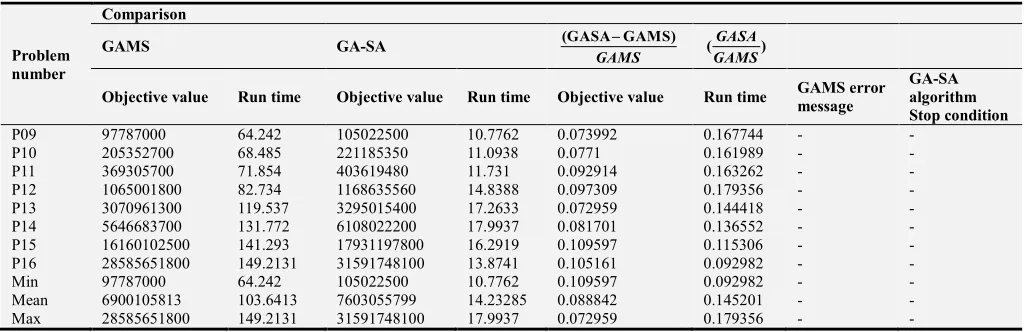
Base on the results of Table 3, in medium sized problem the run time of GAMS optimization software is less than 150s. As it is obvious, hybrid GA-SA algorithm achieved 89% to 92% of the exact optimal solution, within 9% to 18% exact run time. This result denotes the efficiency of the proposed algorithm.
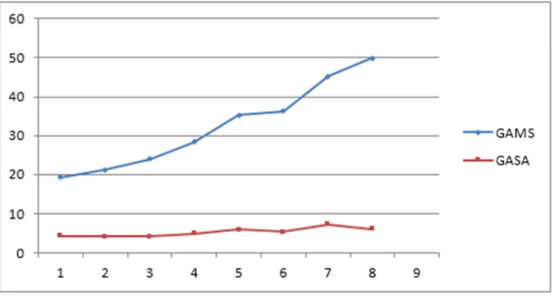
Figure 3 shows, hybrid GA-SA run time versus GAMS run time for medium sized problem. It is observed that the run time and complexity of solving problems by hybrid GA-SA are lower than GAMS optimization software. Besides, the differences between the run time of GAMS optimization software and hybrid GA-SA is increased, as the problem size accelerates. This means that hybrid GA-SA solves the large sized problem in an acceptable time.
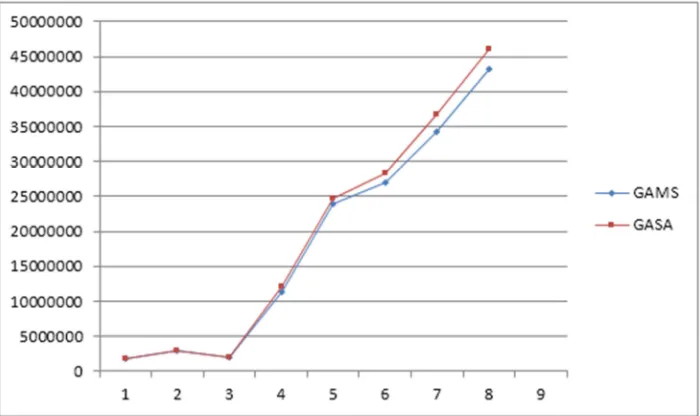
Figure 4 delineates hybrid GA-SA objective values versus GAMS objective value for medium sized problem. The trivial deviation shows the high accuracy of the proposed algorithm to cope with large sized problems.
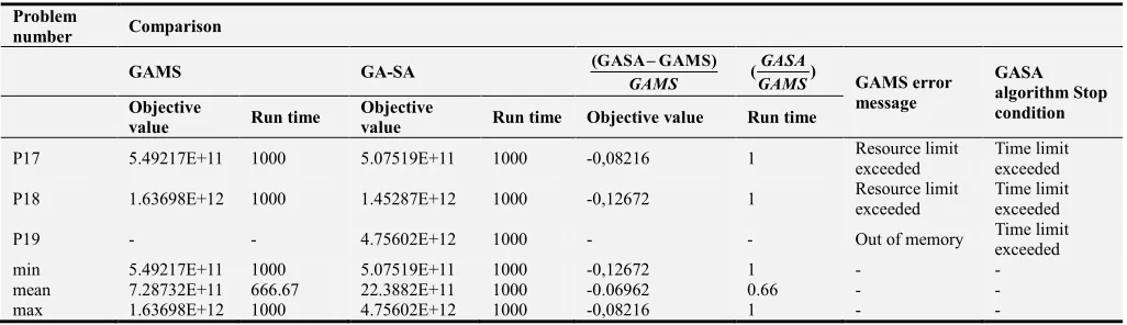
Objective value and run time for GAMS optimization software and hybrid GA-SA for large sized problem are calculated. As shown in Table 4, out of memory message of GAMS appears regarding test problem 19. This is due to the saturation of RAM and stopping the calculation before achieving an acceptable solution.
We also considered 1000s as a limit to stop the algorithm after a specific run time. As it is clear, an error message is appeared in test problem 17 and 18 run by GAMS, which means that the run time exceeded 1000s and GAMS is not able to solve the problem. Furthermore, the proposed hybrid algorithm is not able to converge in considered limit but this algorithm achieved acceptable solution in all 3 test problems. It is observed that, the deviation of hybrid GA-SA from the optimum for test problems 17 and 18 are 8% and 12%, respectively. This denotes the high capability of meta-heuristic algorithms for solving the large sized problem.
Figure 2. Hybrid GA-SA objective value versus GAMS objective value for small sized problem.
Figure 3. Hybrid GA-SA run time versus GAMS run time for medium problem.
Table 1. Some of important inputs for the model.
Inputs Value
c c
αɵ Bernoulli (0.7,{c,c})
Node position of x continuous uniform([0 200],{c}) Node position of y continuous uniform([0 200],{c})
train cc
dis⌢ Euclidean distance
travel cc
tm⌢ disij×continuous uniform([1 3],{c,c})
jct
dem Ceil(continuous uniform([1 5],{j})× continuous uniform([10 200],{c})× continuous uniform([1 5],{t}))
kcf continuous uniform([5 10],{k})
train
cap , ,
( j jct)
j c t
vol dem
K ×
∑
× continuous uniform([0.9 1.2])
j
vol continuous uniform([4 8],{j}))
ϕ
travel cc cc
tm
K
∑
⌢⌢
× continuous uniform([0.5 1.5])
jct
dd Ceil(0.01×disij×continuous uniform([1 3],{i,i}))
cos train k
t continuous uniform([500 1500],{k})×kcf{k}
η 0.01
cos price j
t continuous uniform([1 4],{j})
A Ceil( ,
,
[ ( )]
train
cc jct
i j
train trs man i
k ip
k i p
dis dem
c c c
N K N
+ × + ×
×
∑
∑
∑
∑
⌢
×continuous uniform([0.5 0.8]))
Table 2. Comparison between the performance of GAMS and hybrid GA-SA (optimality and run time) for small sized problem.
Problem number
Comparison
GAMS GA-SA (GASA GAMS)
GAMS
− (GASA)
GAMS GAMS
error message
GA-SA algorithm Stop condition Objective
value Run time Objective value Run time Objective value Run time
P01 1771000 19.232 1771000 4.323 0 0.224782 - -
P02 2941900 21.221 2941900 4.213 0 0.19853 - -
P03 2019900 23.932 2071180 4.196 0.025387 0.221635 - -
P04 11315000 28.382 12092540 4.983 0.068718 0.175569 - -
P05 23879000 35.24 24762360 5.893 0.036993 0.167225 - -
P06 27042000 36.291 28374070 5.362 0.049259 0.156368 - -
P07 34257000 45.234 36677180 7.291 0.070648 0.161184 - -
P08 43188000 49.933 46105930 6.053 0.067563 0.144349 - -
min 1771000 18.932 1771000 4.196 0.070648 0.144349 - -
mean 18523100 27.16278 19349520 5.28925 0.039821 0.171449 - -
max 43188000 45.234 46105930 7.291 0.067563 0.224782 - -
Table 3. Comparison between the performance of GAMS and hybrid GA-SA (optimality and run time) for medium sized problem.
Problem number
Comparison
GAMS GA-SA (GASA GAMS)
GAMS
−
(GASA)
GAMS
Objective value Run time Objective value Run time Objective value Run time GAMS error message
GA-SA algorithm Stop condition
P09 97787000 64.242 105022500 10.7762 0.073992 0.167744 - -
P10 205352700 68.485 221185350 11.0938 0.0771 0.161989 - -
P11 369305700 71.854 403619480 11.731 0.092914 0.163262 - -
P12 1065001800 82.734 1168635560 14.8388 0.097309 0.179356 - -
P13 3070961300 119.537 3295015400 17.2633 0.072959 0.144418 - -
P14 5646683700 131.772 6108022200 17.9937 0.081701 0.136552 - -
P15 16160102500 141.293 17931197800 16.2919 0.109597 0.115306 - -
P16 28585651800 149.2131 31591748100 13.8741 0.105161 0.092982 - -
Min 97787000 64.242 105022500 10.7762 0.109597 0.092982 - -
Mean 6900105813 103.6413 7603055799 14.23285 0.088842 0.145201 - -
Table 4. Comparison between the performance of GAMS and hybrid GA-SA (optimality and run time) for large sized problem.
Problem
number Comparison
GAMS GA-SA (GASA GAMS)
GAMS
− (GASA)
GAMS GAMS error message
GASA algorithm Stop condition Objective
value Run time
Objective
value Run time Objective value Run time
P17 5.49217E+11 1000 5.07519E+11 1000 -0,08216 1 Resource limit exceeded
Time limit exceeded P18 1.63698E+12 1000 1.45287E+12 1000 -0,12672 1 Resource limit
exceeded
Time limit exceeded
P19 - - 4.75602E+12 1000 - - Out of memory Time limit exceeded min 5.49217E+11 1000 5.07519E+11 1000 -0,12672 1 - - mean 7.28732E+11 666.67 22.3882E+11 1000 -0.06962 0.66 - - max 1.63698E+12 1000 4.75602E+12 1000 -0,08216 1 - -
6. Conclusions
A new model for the integration of production and
distribution scheduling in supply chain
management has been developed in this paper which minimizes the costs of transportation and tardiness of delivery a product. We also considered rail transportation to move deteriorating items. A hybrid genetic algorithm-simulated annealing is designed to solve the model for the large-sized problem instances of this mixed integer programming problem. Some small sized and medium-sized test problems have been solved. The results obtain from the hybrid GA-SA satisfactorily compared with results obtained from GAMS optimization software. Some other large-sized test problems have also been solved using the propose hybrid algorithm.
References
[1] Beamon, B. M. (1998). Supply chain design and analysis: Models and methods. International journal of production economics,55 (3), 281-294.
[2] Fahimnia, B., Farahani, R. Z., Marian, R., & Luong, L. (2013). A review and critique on integrated production– distribution planning models and techniques. Journal of Manufacturing Systems, 32 (1), 1-19.
[3] Ghiami, Y., & Williams, T. (2015). A two-echelon production-inventory model for deteriorating items with multiple buyers.
International Journal of Production Economics, 159, 233-240. [4] Goldberg, D. E., 1989. Genetic Algorithms in Search, Optimization and Machine Learning. Addison Wesley Publishing Company, Reading, MA.
[5] Hajiaghaei-Keshteli, M., Aminnayeri, M., & Ghomi, S. F. (2014). Integrated scheduling of production and rail transportation. Computers & Industrial Engineering, 74, 240-256.
[6] Hajiaghaei-Keshteli, M., & Aminnayeri, M. (2014). Solving
the integrated scheduling of production and rail transportation problem by Keshtel algorithm. Applied Soft Computing, 25, 184-203.
[7] Holland, J. H. (1975). Adaption in natural and artificial systems. Ann Arbor MI: The University of Michigan Press. [8] Jakobs, S. (1996). On genetic algorithms for the packing of
polygons. European journal of operational research, 88 (1), 165-181.
[9] Kirkpatrick, S., Gelatt, C. D., & Vecchi, M. P. (1983). Optimization by simulated annealing. Science, 220 (4598), 671-680.
[10] Leung, T. W., Yung, C. H., & Troutt, M. D. (2001). Applications of genetic search and simulated annealing to the two-dimensional non-guillotine cutting stock problem.
Computers & industrial engineering, 40 (3), 201-214. [11] Lundy, M., & Mees, A. (1986). Convergence of an annealing
algorithm. Mathematical programming, 34 (1), 111-124. [12] Maihami, R., & Karimi, B. (2014). Optimizing the pricing and
replenishment policy for non-instantaneous deteriorating items with stochastic demand and promotional efforts. Computers & Operations Research, 51, 302-312.
[13] Pasandideh, S. H. R., Niaki, S. T. A., & Asadi, K. (2015). Bi-objective optimization of a multi-product multi-period three-echelon supply chain problem under uncertain environments: NSGA-II and NRGA. Information Sciences, 292, 57-74. [14] Priyan, S., & Uthayakumar, R. (2014). Two-echelon
multi-product multi-constraint multi-product returns inventory model with permissible delay in payments and variable lead time. Journal of Manufacturing Systems.
[15] Saracoglu, I., Topaloglu, S., & Keskinturk, T. (2014). A genetic algorithm approach for multi-product multi-period continuous review inventory models. Expert Systems with Applications, 41 (18), 8189-8202.
[16] Yaghini, M., & Akhavan, R. (2012). Multicommodity network design problem in rail freight transportation planning.
Procedia-Social and Behavioral Sciences, 43, 728-739. [17] Zhang, J., Liu, G., Zhang, Q., & Bai, Z. (2015). Coordinating