Semi-Analytical and Numerical Solution of Regularized Burdet Equations to Predict the Motion of an Artificial Satellite

(1)

Published online June 20, 2014 (http://www.sciencepublishinggroup.com/j/ajam) doi: 10.11648/j.ajam.20140203.13

Semi-analytical and numerical solution of regularized

Burdet equations to predict the motion of an artificial

satellite

Hany R. Dwidar

Astronomy, Meteorology and Space Science Dept., Faculty of Science - Cairo University, Giza, Egypt

Email address:

[email protected]

To cite this article:

Hany R. Dwidar. Semi-Analytical and Numerical Solution of Regularized Burdet Equations to Predict the Motion of an Artificial Satellite.American Journal of Applied Mathematics. Vol. 2, No. 3, 2014, pp. 85-91. doi: 10.11648/j.ajam.20140203.13

Abstract:

In this paper, literal analytical solution in power series forms which is one of the semi-analytical solution, are developed for the regularized Burdet equations to estimate the motion of an artificial satellite under the influence of J2-Earth’s

gravitational field. Also a numerical solution of the regularized Burdet equations is applied using eighth order Dormand-Prince Rung-Kutta method. Comparison between the power series solution and the numerical solution applied to high eccentric frozen satellite orbit is also given and showed excellent agreement.

Keywords:

Astrodynamics, Satellite Orbit Determination, Power Series, Numerical integration

1. Introduction

It is well known that the solutions of the Classical Newtonian Equations of motion are unstable and these equations are not suitable for long-term integrations. Many transformations have emerged in the literature in the recent past to stabilize the equations of motion either to reduce the accumulation of local numerical errors or allowing of using a larger integration step size, in the transformed space, or both ([9] , [1] and [6]). One of such transformation, known as the Sperling/Burdet Equations, is due to [17] and [3] who regularized the non-linear Kepler motion and reduced it to linear differential equations of a harmonic oscillator of constant frequency. Reference [5] outlined the differential equations and the initial value problem together with the transformation to rectangular coordinates and classical elements. The Burdet’s variables can be adopted for the computation of elliptic, parabolic and hyperbolic motion ([13]). References [12] , [1] and [6] applied this method numerically to predict a satellite motion.

In spite of their advantages in many cases, analytical methods do not always provide high-accuracy solutions to orbital problems, as required. Both analytical and semi-analytical methods use an analytical transformation to produce mean, slowly varying differential equations ([2] , [14] , [15] and [16]). However, analytical solutions, though difficult to obtain for complex force models and limited to relatively simple models, represent a manifold of solutions

for a large domain of initial conditions and parameters and find indispensable application to mission planning and qualitative analysis. Otherwise power series solution (which of course assumed to be convergent) can serve as the analytical representation of its solution. Moreover, it is worth noting that the power series is one of the most powerful methods of mathematical analysis when the problems are to be studied on computers. In fact, most computers often use series in the calculations of the majority of the elementary functions.

For the numerical solution, We have the Dormand–Prince method, which is an explicit method for solving ordinary differential equations ([4]). The method is a member of the Runge–Kutta family of ODE solvers and its eighth order uses 12 function evaluations with err = O(h8) where h is the step size ([8] and [10]) .

In this paper, we construct a recurrent power series solution for the Sperling-Burdet perturbed differential equations of motion depending on Taylor series expansion to get the classical elements of the satellite at any time. We apply the eighth order Dormand-Prince method to these equations to get the numerical solution and compare this solution with the power series solution.

2. Formulation of the Problem

(2)

3

µ

x

T

r

+

=

ɺɺ

(1)

where

x

is the relative position vector,

r

=

x

, µ is

the Earth's gravitational constant, T is the all perturbing

forces, which equals to _

     ₊ ∂ ∂

− _P*

x

V _{, where} *

P

is

the resultant of all non-conservative perturbing forces, and V

is the perturbed time-independent potential, which can be expressed as

(

)

1

3 2

1 /

i

(

)

i

i i

i

V

µ

R J

r

L x / r

∞ ₊

⊕ =

=

∑

where R⊕ is the Earth's equatorial radius, Ji is the

non-dimensional coefficient of the Earth's potential and Li is

the Legendre polynomial of order i ([11]).

In our case the only force acting on an artificial satellite

is that due to the Earth's oblateness, so we have

,

P

*

0 =

(2.1)

5 2 5 2 3 2 2 1 2

3 ₋ ₋

−

= q x r q r

V (2.2)

where q2 = µ

R

_⊕2J2 and

2 3 2 2 2

1

x

r

=

+

.

Eq. (1) are the basic classical equations of motion of artificial satellites and the corresponding perturbed equations of motion with the independent variable (true anomaly) in terms of the Burdet’s parameters ([5] and [12]) are

(

ξ

)

ξ

µ

ξ

′′+ = −1_p−1_u−3_T−<_T > − _p−1_p′ ′

2 1

, , (3.1)

( )

p

(

p

u

)

T

( )

p

u

′′

+

=

−1

−

µ

2 −1

<

,

ξ

>

−

2

−1

′

, (3.2)

(

)

< ′>

=

′ −

ξ

µ ,

2 _u3 1 _T

p , (3.3)

2 2 / 1

)

(

− −

=

′

p

u

t

µ

, (3.4)

where

r

u

=

1 /

,

x

u

r

x

=

/

ξ

;

(

2

)

2

,x r

x r

p _ < ɺ ɺ > −ɺ      = µ ,

and *

P x

V T = − ∂ +

∂ ;

Hence < a,b > is used to denote the scalar product of two vectors

a

and b . Denoting differentiation with respect to the new time f (true anomaly) by a prime ('), since

the independent variable is changed from time (t) to new time (f) according to

2

r p dt

df ₌ µ _,

([3] and [12]).

After transform Eqs (3) into ten first order differential equations, we get

4

1

g

′

=

, (4.1)

5

2

g

′

=

, (4.2)

6

3

g

′

=

, (4.3)

( )

{

[

]

}

9 4

1 9 3 3 2 2 1 1 1 1 3 7 1 9 1

4 g g g T g Tg T g Tg 0.5g g g

g′=− +

µ

− − − + + − − ′ ,

(4.4)

( )

{

[

]

}

9 5

1 9 3 3 2 2 1 1 2 2 3 7 1 9 2

5

g

T

g

T

g

T

g

T

g

0 .

5 g

g

′

=

−

+

µ

− −

−

+

−

′

,

(4.5)

( )

{

[

]

}

9 6

1 9 3 3 2 2 1 1 3 3 3 7 1 9 3

6 g g g T g T g T g T g 0.5g g g

g′=− + µ − − − + + − − ′ , (4.6)

8

7

g

′

=

, (4.7)

(

)

{

}

9 8

1 9 3 3 2 2 1 1 2 7 1 9 1 9 7

8 g g g g T g T g T g 0.5g g g

g′=− + − − µ − − + + − − ′ , (4.8)

(

) {

1 4 2 5 3 6

}

1 7

9 2 g T g T g T g

g′ = µ − + + , (4.9)

(

)

1/2 9 2 7 10 − −

=

′

g

µ

. (4.10)

where

i i i

g

= =

ξ

ux

,

g

_i₊₃

=

ξ

_i

′

, i = 1, 2, 3;

u

g

₇

=

,

u

g

₈

=

′

,

∗

=

p

g

₉ ,

and

g

₁₀

=

t

.

and we have from Eq. (2.2)

(

)

2 4 2

1 2 1 7 3

3

5

1

2 T

=

µ

J

R

⊕

g g

g

−

, (5.1)

(

)

2 4 2

2 2 2 7 3

3

5

1

2 T

=

µ

J R g g

_⊕

g

−

; (5.2)

(

)

2 4 2

3 2 3 7 3

3

5

3

2 T

=

µ

J

R

_⊕

g g

g

−

. (5.3)

3. Recurrent Power Series Solution

(3)

3.1. Auxiliary dependent variables

Let us define the following auxiliary dependent functions, which transform the system of differential equations of motion in a new system of differential equations where all denominators have been removed, as well as all the powers of

g

_i.

7 7

1

g

a

=

;

a

₂

=

a

₁

a

₁;

3 3

3

g

a

=

; 2

2

3 2

Q = µ J R_⊕ ;

2

1, 2, 3

i i

f

=

g a

i

=

;

f

_i₃

=

f a

_i ₃

i

=

1, 2, 3

;

1 13

1

5 Q

f

Q

f

t

=

−

; t₂ = 5Q f_{2 3} −Q f₂;

3 33

3

5 Q

f

3 Q

f

t

=

−

;

6 1 1 2 2 3 3

b

=

t g

+

t g

+

t g

;

6

1, 2, 3

i i

y

=

b g

i

=

;

1, 2 , 3

ii i i

y

=

t

−

y

i

=

;

7 1

7

11

g

1 /

g

=

−

=

;

g

_{1 2}

=

g

_{1 1}

g

_{1 1};

1 3 1 1 12

g

=

g

;

g

₁₄

=

g

₉−1

=

1 /

g

₉;

1/ 2

15 9

1 /

9

g

=

g

−

=

g

;

g

₁₆

=

g

₁₅

g

₁₂ ;

4 1 4 2 5 3 6

b

=

t g

+

t g

+

t g

;

b

₅

=

g

₁₃

b

₄;

14 13

17

g

=

;

g

₁₈

=

b

₅

g

₁₄ ;

7i 17 ii

1, 2, 3

g

=

g

y

i

=

;

8i 18 i

4, 5, 6

g

=

g

i

=

;

and

19 1 4 1 2

g

=

g

;

g

₂₀

=

g

₁₉

b

₆;

g

₂₁

=

g

₈

g

₁₈ ; Using the previous substitutions into Eqs.(4), we get the following first order differential set in ten unknowns

4

1

g

′

=

, (6.1)

5

2

g

′

=

, (6.2)

6

3

g

′

=

, (6.3)

84 71 1 4 1 1 g g g g

µ

− + − =

′ ; (6.4)

85 72 2 5 1 1 g g g g µ µ − + − =

′ ; (6.5)

86 73 3 6 1 1 g g g g

µ

− + − =

′ ; (6.6)

8

7 g

g ′ = ; (6.7)

21 20 14 7 8 1 1 g g g g g µ µ − − + − =

′ ; (6.8)

5 9 2 b g µ =

′ ; (6.9)

16 10 1 g g µ =

′ _{. (6.10)}

3.2. Power series manipulations

Let us define the ten Taylor expansions as follows

0

(n) n

i i

n

h

H

f

∞

=

∑

; i = 1, 2, …, 10 (7)

and

1

0

(

1)

(n ) n

i i

n

h

n

H

f

∞

+

=

′ =

∑

+

; (8)

where we have used small letters (h) for the unknown variables and capital letters (H) for the coefficients in their Taylor series expansion.

Now, let us define a and b as two convergent power series such that

0 (i) i

i

a A s

∞ = =

∑

, 0 (i) i i

b B s

∞

=

∑

.

Then, we have (Gradshteyn and Ryzhik, 2007)

• Division of power series

( ) ( 0 )

1

1 k k

k b C s a A ∞ = =

∑

where

(0) (0) ( ) ( ) ( ) ( )

(0) 1

1

, k k k i i 1,2,...

i

C B C B C A k

A

∞ −

=

= = −

∑

=

• Power series raised to powers

( )

0 0

n

n ( i) i i i

i i

a A s P s

∞ ∞ = =   =   = 

∑



∑

where

(0) (0) ( ) ( ) ( )

(0) 1

1

( ) , ( ) 1

k

n k k i i i

P A P in k i P A k kA

− =

= =

∑

− + ∀ ≥

• Multiplication of power series

0

( n ) n n

c a b C s

∞ = = =

∑

, where 0 n

(n ) (i) ( n - i) i

C A B

=

∑

.

Substituting Eqs .(7) and (8) into Eqs.(6), and using the above rules for the power series, and equating coefficients of equal powers of f in both sides of each of the resulting equations, then we get the coefficients of the following recurrence formulae ) ( 4 ) 1 ( 1 n n

G

n

+

=

; (9.1)

) ( 5 ) 1 ( 2 n n G G

(4)

) ( 6 ) 1 ( 3 n n

G

n

+

=

; (9.3)

) ( 84 ) ( 71 ) ( 1 ) 1 ( 4 1

1 n n

n

n _G _G _G

G n µ µ − + − = +

; (9.4)

) ( 85 ) ( 72 ) ( 2 ) 1 ( 5 1

1 n n

n n G G G G n

µ

− + − = +

; (9.5)

) ( 86 ) ( 73 ) ( 3 ) 1 ( 6 1

1 n n

n

n _G _G _G

G n µ µ − + − = +

; (9.6)

) ( 8 ) 1 ( 7 n n

G

n

+

=

; (9.7)

) ( 21 ) ( 20 ) ( 14 ) ( 7 ) 1 ( 8

1

n n

n

_G

G

n

µ

−

+

−

=

+

; (9.8)

) ( 5 ) 1 ( 9 2 n n B G n µ = +

; (9.9)

) ( 16 ) 1 ( 10 1 n n G G n µ = +

. (9.10)

then we can compute the coefficients (capital letters) to get small letters which are the unknown variables (g’s).

4. Computational Developments

In this section, the computational developments of the formulation of section 3for power series will be considered. For the eighthorder Dormand-Prince method will be applied on the first differential Eqs (4).

4.1. Computation Of The Initial Values:

Knowing the classical elements {a e M, , , ,i ω Ω, } at some

time t0(corresponding to f0 ), we can get the position

vector x₀ and the velocity vector xɺ0 at the same time

0

t ([18]), where

a

is a semi major axis, e is an eccentricity, Mis a mean anomaly,

i

is an inclination, ωis an argument of perigee and Ω is a longitude of the ascending node.

Now we can compute

2 03 2 02 2 01

0 x x x

r = + + , and rɺ0=(1/ )(r0 x x01ɺ01+x x02ɺ02+x x03ɺ03).

and we can get g’s as follows

0 0

0 x /r

g i = i ,

09 , 0 0 , 0 0 3 ,

0 (r x r x )/ g

g _i₊ = ɺ _i − ɺ _i µ , i = 1, 2, 3;

0 07

1 /

r

g

=

,

09 0

08 r / g

g =− ɺ µ ,

),

(

)

/

(

₀2 ₀₁2 ₀₂2 ₀₃2 ₀2

09

r

x

r

g

=

µ

ɺ

+

ɺ

+

ɺ

−

ɺ

and

g

₁₀

=

t

₀.

Vice versa, the position and velocity are obtained from the

g’s as the following relations

7

/

g

x

_i

=

_i , and xɺi =(g g₇ i+₃−g g₈ i) µg₉ .

Finally, we get the classical elements from the position

vector

x

₀ and the velocity vector xɺ₀ at the same time

t

([18]).

4.2. The accuracy check

The accuracy of the computed values of the g's variables at any new time f (corresponding to the time t) could be checked by the two following relation

2 2 2

1 2 3 1

g +g +g = , and g g₁ ₁′+g g₂ ₂′+g g₃ ₃′=0.

4.3. Utilization

When the true anomaly f is sufficiently large, we may (as usually done for all initial value problems) divide the interval f into some intervals into some intervals each of short length, e.g. the ( f - f₀) may be divided into (r-l) intervals : ( f₁− f₀), ( f₂− f₁), ..., ( f − f_q) such that (fh− fh−₁)≪(f − f₀). Then solve the initial value problem for the first interval to find the solution at the value

j

f . The solution at f_j could then be used as the initial condition for the second interval and so on. By this artifice one usually needs small number of the coefficients for the power series representation in each interval.

4.4. The step size ∆∆∆∆f

The step size of the new time ∆f could be computed from the corresponding step size ∆t of the ordinary time as

2 µ p ∆f ∆t r = .

4.5. Numerical test

In what follows the results of a comparison between the power series solution and the numerical integration of the first differential Equations 3 will be given. We use the following two line elements for MOLNIYA satellite which is highly eccentric frozen satellite orbit, as the initial conditions (www.spacetrack.com) at epoch 06 May 2014.

0 MOLNIYA 1-93

1 28163U 04005A 14115.76724197 .00000117 00000-0 00000+0 0 3266

2 28163 064.4633 083.5168 7312151 246.9027 252.2464 02.00655253 74609

We calculate the recurrent power series up to ten step

(N=10), while the step size is 2 500

h= π , for 1000 cycle of the satellite. The adopted physical constant are R_⊕ = 1 e.r. (earth radii), µ = 0.0055302632857476 e.r.3/min2 , and the Earth’s zonal harmonic coefficient J2 equal 1.0826157×10-3.

(5)

Fig. 1. Comparison between numerical and analytical solutions for the semi-major axis

Fig. 2. Comparison between numerical and analytical solutions for the eccentricity

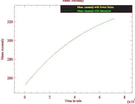
Fig. 3. Comparison between numerical and analytical solutions for the mean anomaly

Fig. 4. Comparison between numerical and analytical solutions for the inclination

Fig. 5. Comparison between numerical and analytical solutions for the argument of perigee

(6)

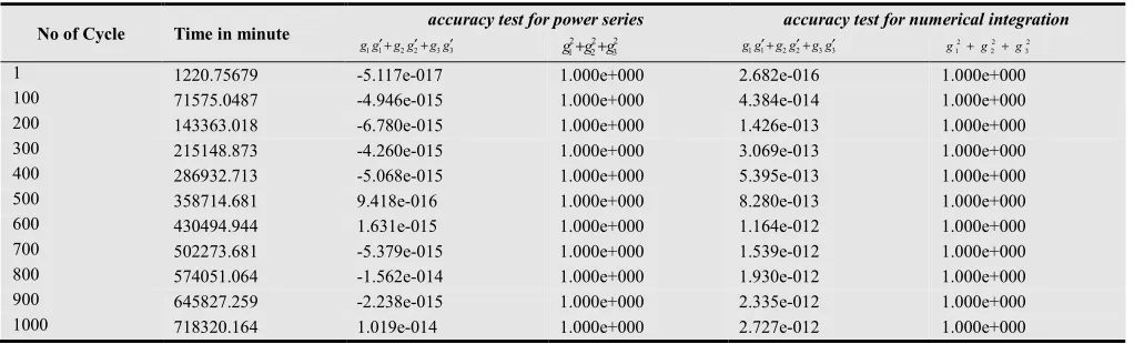
Table 1. The accuracy check

No of Cycle Time in minute accuracy test for power series accuracy test for numerical integration

11 2 2 33

g g′+g g′+g g′ 2 2 2 1 2 3

g g g+ + g g11′+g g2 2′+g g3 3′

2 2 2

1 2 3

g +g +g

1 1220.75679 -5.117e-017 1.000e+000 2.682e-016 1.000e+000

100 71575.0487 -4.946e-015 1.000e+000 4.384e-014 1.000e+000

200 143363.018 -6.780e-015 1.000e+000 1.426e-013 1.000e+000

300 215148.873 -4.260e-015 1.000e+000 3.069e-013 1.000e+000

400 286932.713 -5.068e-015 1.000e+000 5.395e-013 1.000e+000

500 358714.681 9.418e-016 1.000e+000 8.280e-013 1.000e+000

600 430494.944 1.631e-015 1.000e+000 1.164e-012 1.000e+000

700 502273.681 -5.379e-015 1.000e+000 1.539e-012 1.000e+000

800 574051.064 -1.562e-014 1.000e+000 1.930e-012 1.000e+000

900 645827.259 -2.238e-015 1.000e+000 2.335e-012 1.000e+000

1000 718320.164 1.019e-014 1.000e+000 2.727e-012 1.000e+000

5. Conclusion

From the figures we can conclude that, from the initial up to 500 mean solar days, there are obviously changes in the two elements (Ω, M), but the other elements (a, e, i) show lightly change, for the numerical integration and power series solutions. This expected because the only force affecting on the motion of artificial satellite is Earth’s gravitational field (J2), so the elements Ω, M behaviors are

secular while the elements a, e, i have periodic treatment. But ω has very slightly change, as expect, because this satellite is frozen orbit (Molniya).

Also, the table shows the accuracy check for the two methods of solutions which one of them is always nearly to zero and the other is exact one, i.e., the predictions of the components of position and velocity (the elements) of the artificial satellite is very good.

The figures show that the comparison between the two methods, power series and numerical integration are identical. But the table of accuracy check show that the power series method is more accurate than the numerical integration. We can conclude the efficiency of the power series method.

To get more accurate prediction of the motion of the artificial satellite we will be taken into account the whole other forces affecting on the motion.

References

[1] I. Aparicio and L. Floria, "A BF-regularizationof a nonstationary two-body problem under the Maneff perturbing potential," Extracta Mathematicae, vol. 12, no. 3, 1997.

[2] R. Broucke, "Solution of the N-Body Problem with Recurrent Power Series," Celestial Mechanics, vol. 4, pp. 110-115, Sep. 1971.

[3] C. A. Burdet, "Regularization of the two body problem,"

Zeitschrift für angewandte Mathematik und Physik, vol. 18, no. 3, pp. 434-438, 1967.

[4] J. R. Dormand and P. J. Prince, "A Family of Embedded Runge-Kutta Formulae," Journal of Computational and Applied Mathematics, vol. 6, p. 19–26, 1980.

[5] W. Flury and G. Janin, "Accurate integration of geostationary orbits with Burdet's focal elements," Astrophysics and Space Science, vol. 36, pp. 495-503, Sep. 1975.

[6] T. Fukushima, "Numerical Comparison of Two-Body Regularizations," The Astronomical Journal, vol. 133, no. 6, pp. 2815-2824, Jun. 2007.

[7] I. S. Gradshteyn and I. M. Ryzhik, Table of Integrals, Series, and Products, Seventh Edition ed., A. Jeffrey and D. Zwillinger, Eds., New York: Academic Press Inc., 2007.

[8] E. Hairer, S. P. Nørsett and G. Wanner, Solving Ordinary Differential Equations I (Nonstiff Problems), Third ed., Springer-Verlag, 2008.

[9] D. J. Jezewski, "A Comparative Study of Newtonian, Kustaanheimo/Stiefel, and Sperling/Burdet Optimal Trajectories," Celestial Mechanics, vol. 12, no. 3, pp. 297-315, Nov. 1975.

[10] W. H. Press, S. A. Teukolsky, W. T. Vetterling and B. P. Flannery, NUMERICAL RECIPES The Art of Scientific Computing, Third Edition ed., Cambridge: CAMBRIDGE UNIVERSITY PRESS, 2007.

[11] M. A. Sharaf and M. E. Awad, "Prediction of trajectories in Earth's gravitational field with axial symmetry.," Proc. Math. Phys. Soc. Egypt, vol. 60, 1985.

[12] M. A. Sharaf, M. R. Arafah and M. E. Awad, "Prediction of satellites in earth's gravitational field with axial symmetry using Burdet's regularized theory," Earth Moon and Planets,

vol. 38, pp. 21-36, May 1987.

[13] M. Silver, "A short derivation of the Sperling-Burdet equations," Celestial Mechanics, vol. 11, no. 1, pp. 39-41, Feb. 1975.

[14] G. Sitarski, "Recurrent power series integration of the equations of comet's motion," Acta Astrono., vol. 29, no. 3, pp. 401-411, 1979.

(7)

[16] G. Sitarski, "Solution of the ADONIS problem," Acta Astrono., vol. 29, no. 3, pp. 413-424, 1979.

[17] H. Sperling, "Computation of Keplerian Conic Sections,"

American Rocket Society Journal, vol. 31, no. 5, pp. 660-661, 1961.