Published online April 2, 2013 (http://www.sciencepublishinggroup.com/j/ijepe) doi: 10.11648/j. ijepe.20130202.12
A novel numerical scheme for a scale-invariant form of
equation of motion: development of solver and
application to engineering flow problems
Bo Wan*, F.-K. Benra, H. J. Dohmen
Department of Mechanical Engineering, Faculty of Engineering Sciences, University of Duisburg-Essen, Duisburg 47048, GERMANY
Email address:
[email protected] (Bo Wan)
To cite this article:
Bo Wan, F.-K. Benra, H. J. Dohmen. A Novel Numerical Scheme for a Scale-Invariant Form of Equation of Motion: Development of Solver and Application to Engineering Flow Problems, International Journal of Energy and Power Engineering. Vol. 2, No. 2, 2013, pp. 37-45. doi: 10.11648/j.ijepe.20130202.12
Abstract:
The goal of the current paper is to describe an in-depth study of a numerical implementation of the modified equation of fluid motion for incompressible flow. The applications of the developed solver are discussed for both laminar and turbulent flow problems. The results are evaluated by comparing them with those obtained by other methods, including the numerical results obtained by the Navier–Stokes solver measurement data. Then, the computational effort and accuracy of the solver are emphasized. The comparisons indicate that the developed solver, which is based on the modified equation of fluid motion, requires less computation time than the Navier–Stokes solver, and it produces physically reasonable results validated by measurement data.Keywords:
Modified Equation of Fluid Motion, Statistical Mechanics, CFD, Incompressible Flow, Navier–Stokes Equa-tions, Navier–Stokes Solver, Flat Plate, Airfoil, Curved Duct1. Introduction
During the past several decades, there has been steady progress in the field of computational fluid dynamics (CFD) methodologies. This progress has allowed engineers and designers in the turbomachinery industry to gain deeper insights into the effects of fluid dynamics on design processes used in the field of turbomachinery. The funda-mental governing equations for solving most CFD prob-lems are the Navier–Stokes equations. The primitive varia-ble formulations of these equations result in the derivation of a large system of non-linear algebraic equations after finite volume method (FVM) discretization is carried out. However, these equations impede the development of nu-merical solutions for the Navier–Stokes equations. Hence, it is assumed that engineers would be interested in another equation that does not have non-linear properties.
On the basis of the scale-invariant theory of statistical mechanics, Sohrab [1, 2] introduced a linear equation termed the “scale-invariant form of the equation of fluid motion” or the “modified equation of fluid motion”. Pre-liminary investigations have shown that this modified
equ-ation can be extended to solve incompressible flow prob-lems. Several basic flow models were analytically devel-oped using this equation. Consequently, satisfactory corre-lation between the estimated and experimental data was achieved. This result then stimulated further applications of this modified equation in the development of CFD codes to obtain more numerical solutions of turbomachinery prob-lems.
The use of the physical linear characteristic of the aforementioned modified equation of fluid motion helped us develop a novel numerical solver to solve CFD prob-lems. The detailed methodology of the developed solver has been discussed by Wan et al [3]. The improved algo-rithms simplify the velocity iteration procedure and reduce numerical oscillation during solver execution. By simulat-ing a fundamental laminar flow problem, the developed solver, which is named as the Sohrab solver, delivers phys-ically reasonable results and consumes less computational resources than that consumed by the solver that uses the Naiver–Stokes equations.
dimensional (3D) curved duct models. The results obtained by the Sohrab solver were evaluated by comparing them with the numerical solutions obtained by the Navier– Stokes solver and valid experimental data.
2. Modified Equation of Fluid Motion
and Modified Turbulence Theory
Recently, Sohrab [2] introduced the derivation of the modified equation of fluid motion for incompressible flow using a scale-invariant definition of the convective velocity w 2 p t β β β β β β β υ ρ ∇ ∂ + ∇ − ∇ = −
∂ U w U U (1)
Comparing Eq. (1) with the Navier–Stokes equations for incompressible flow, we get
2 p t β β β β β β β υ ρ ∇ ∂ + ∇ − ∇ = −
∂ U U U U (2)
It is obvious that convective velocity wβ can replace the
local velocity Uβ in the second term on the left–hand side
of the equation. This important feature of the modified eq-uation of fluid motion eliminates its non–linearity.
As discussed by Sohrab in [4], the potential energy of a fluid can be expressed in term of peculiar velocity as fol-lows:
2
β β β
ε =ρ ′v (3)
This energy is responsible for the stability of clusters or particles in a fluid. Under a particular condition, the local velocity at the β+1 scale Uβ+1 can be increased to equal
that at β scale Uβ. In other words,
1 1
β+ = β = β+
U U u (4)
Thus, peculiar velocity can be eliminated as
1 1 1 0
β+ β+ β+
′ = − =
v u U (5)
Further, potential energy at the corresponding scale can be subsequently eliminated as
2
1 1 1 0
β β β
ε + =ρ +v′+ = (6)
Such elimination of the peculiar velocity and potential energy on the laminar scale will result in the instability of fluid elements and the transition of the entire fluid field to a fully turbulent field consisting of eddy dynamics on a low scale.
Consequently, in the following solutions, convective locity at the turbulence scale is derived from the local ve-locity at the laminar scale as
turbulence= laminar
w U (7)
3. Applications of the Sohrab Solver
The developed solver based on the modified equation of fluid motion is named as the Sohrab solver. Following the methodology of this novel solver [3], the simulations of several flow models are discussed to explain the applica-tions of the solver in this section. First, an airfoil model will be discussed for both the laminar and turbulent flow environments to describe the procedure for deriving con-vective velocity. Second, the simulation of turbulent flow over a flat plate, which can be considered as an extension of the calculation model in [3], will be discussed. Finally, under different geometric conditions, the calculation of turbulent flow in a 3D curved duct will be discussed to confirm the ability of the Sohrab solver to calculate turbu-lent flow for a 3D case as well.
3.1. Airfoil Simulation
An airfoil model was chosen as the model for carrying out numerical simulations under both the laminar and tur-bulent flow environments using the Sohrab solver to con-firm its application to calculate turbulent flow. The ob-tained results are validated by comparing them with those obtained by the classical Navier–Stokes solver and valid measurement data.
3.1.1. Model
The model used for the simulation was obtained from the experiments of A. Thom and P. Swart [5]. The geome-tric profile of the model used in this study is a modified version of the classical two-dimensional (2D) Royal Air Force (RAF) 6a airfoil, which has square ends on both the sides because of poor manufacturing techniques practiced in 1940, when this airfoil was first constructed.
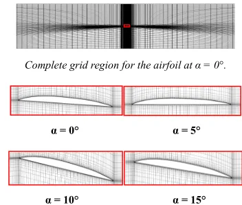
The grids of the entire calculation region and detailed structure around the airfoil are shown in Fig. 1. The total grid number is about 58,000, and four mesh models that correspond to different angles of attack are developed for the numerical simulations discussed further.
Complete grid region for the airfoil at α = 0°.
α = 0° α = 5°
α = 10° α = 15°
Fig. 1. Grids of different angles of attack.
3.1.2. Laminar Flow
the laminar flow field:
laminar = potential
w U (8)
Consequently, the convective velocity field can be con-structed by executing potentialFOAM, which is a special solver available with the OpenFOAM application for solv-ing only Euler equation.
As shown in Fig. 2, the calculated velocity field simply follows the airfoil profile, and any viscous effect is ignored. The variation in the velocity magnitude is caused by the effect of the continuity equation.
Fig. 2. Potential flow around airfoil.
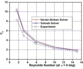
The drag coefficient is defined as
2 1 2
d d
F C
cl
ρ
=
U (9)
Using this definition, the calculated drag coefficients versus different Reynolds numbers at an angle of attack α = 0° obtained using both the Navier–Stokes and the Sohrab solvers are compared with the experimental data, as shown in Fig. 3. The numerical results of the drag coefficient tained by the Sohrab solver simply coincide with that ob-tained by the classical Navier–Stokes solver, and exhibit the same trend as that exhibited by the results obtained by the Navier–Stokes solver: the Reynolds number increases with a reduction in the drag coefficient. A large difference is found between the experimental data and the estimated numerical results, and this difference decreases as the Rey-nolds number increases. The phenomenon observed here has remained unsolved in the case of numerous numerical CFD codes. For a low Reynolds number, the numerical results of the drag coefficient are always higher than the experimental results.
Fig. 3. Drag coefficients for different Reynolds numbers under a laminar
flow.
Similarly, Fig. 4 illustrates the variations in the drag coefficient versus different angles of attack. The simulation results shown in this figure are obtained for several Rey-nolds numbers, because each angle in the experiment coin-cided with a particular Reynolds number. Fig. 3 and Fig. 4 clearly show that the results calculated by the Sohrab solv-er are in good agreement with those calculated by the clas-sical Navier–Stokes solver and experiment results. Howev-er, the experimental data greatly differs from the numerical results at very low Reynolds numbers and large angles of attack. This difference can be attributed to the aforemen-tioned numerical reasons and the measurement error intro-duced into the experiment owing to poor manufacturing techniques practiced in 1940.
Fig. 4. Drag coefficients for different angles of attack under a laminar
flow (Re≤15).
3.1.3. Turbulent Flow
In section 2, a transition from the laminar to the turbu-lence scale was discussed to derive the convective velocity relation in Eq. (7). This transition allows us to use the So-hrab solver to solve the turbulent flow problem. By using the velocity field constructed using the laminar flow as convective velocity, the Sohrab solver is applied for the airfoil model under turbulence boundary conditions. Be-cause no experimental data is available, we can compare the results of the drag coefficient calculated by only the Sohrab and Navier–Stokes solvers. The Reynolds number is set to Re = 100,000, and water at 25℃ is used as the
media for carrying out the simulation. Various angles of attack are calculated to compare different results obtained using the two numerical solvers.
Fig. 5. Drag coefficients for different angles of attack under a turbulent flow.
Fig. 6. Velocity field constructed using the Navier–Stokes solver.
Fig. 7. Velocity field constructed using the Sohrab solver.
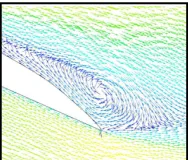
As discussed in [3], an unstable Peclet number leads to velocity oscillation during the iteration process in the ex-ecution of the Navier–Stokes solver. In certain cases, this oscillation may be not totally damped during numerical iteration, thus affecting the flow field. In physics, a vortex induced by numerical oscillation contains considerable amount of kinetic energy and decays rapidly through the action of fluid viscosity. According to [6], the presence of a trailing vortex further affects the airfoil, and this effect would result in the increase in drag force and the conse-quent reduction in lift force. Hence, as shown in Fig. 5, at α = 15°, the drag coefficient calculated by the Sohrab solver is less than that calculated by the Navier–Stokes solver.
Fig. 8 shows the pressure around the airfoil. The figure clearly shows that the pressure difference calculated by the Sohrab solver is smaller than that calculated by the Navier– Stokes solver, particularly at the trailing edge of the airfoil. This result corresponds to the induction of the vortices shown in Fig. 6 and Fig. 7, thus further explaining the drag coefficient differences observed in Fig. 5. Further, the ve-locity gradients inside the boundary layer for Points 1 and 2 on the airfoil upper surface, which are illustrated in Fig. 8, are compared. Fig. 9 shows that at point 1, which is close to the leading edge, the velocities calculated by both the solvers coincide well with each other. However, at Point 2, which is close to the trailing edge, the effects of the trailing vortex result in a considerable difference in the velocity
distribution. Therefore, at small angles of attack when no vortex is present in the flow field, the Sohrab solver can deliver results similar to those delivered by the Navier– Stokes solver, whereas as the angle of attack increases, the vortex begins to strongly affect both the pressure and ve-locity fields, leading to a large difference between the solu-tions obtained by both the solvers.
Fig. 8. Pressure around the airfoil.
Fig. 9. Velocity gradients in the boundary layer.
Following the calculation procedure of the Sohrab solver in the case of the airfoil model, we recognized the need to calculate the corresponding convective velocity in order to perform turbulence simulations. In detail, numerical simu-lation initiates by obtaining the potential flow solution and continues with the calculation of the laminar flow. This procedure can be considered as the initial condition of the turbulence calculation that would follow the calculation of laminar flow. On the other hand, in the case of the Navier– Stokes solver, the same procedure is assumed to initiate turbulence calculation with a smooth initial condition in OpenFOAM [7]. Therefore, in order to compare the calcu-lation time taken by the two solvers, the aforementioned initial process can be ignored and only the turbulence cal-culation process should be carried out.
3.2. Turbulent Flow over a Flat Plate
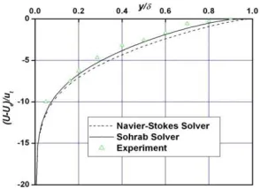
By using the results of the laminar calculation in [3], this section discusses the application of the Sohrab solver to the calculation of turbulent flow over a flat plate. Using the physical boundary condition described in the Schultz– Grunow experiment [8], both the Navier–Stokes and So-hrab solvers are applied to calculate the turbulent flow.
boundary layer are compared with the experimental data in Fig. 10.
Fig. 10. Comparison of measurements and numerical results for turbulent
flow over flat plate.
As shown in Fig. 10, the complete velocity profile shape constructed using the Sohrab solver is slightly higher than that constructed using the Navier–Stokes solver, and the entire shape of the former exactly coincides with the latter. In terms of the measurement data points, the Sohrab solver results are confirmed to be closer to the data points than the Navier–Stokes solver results. Thus, this result confirms the accuracy of the Sohrab solver in calculating turbulent flow. Furthermore, it offers a numerical explanation for the re-sults obtained in section 2.
3.3. Curved Duct
In the previous sections, two classical flow models were simulated by using the Sohrab solver, and the results were found to be in good agreement with those obtained by the Naiver–Stokes solver. Such encouraging results further stimulated us to carry out numerical investigations into the Sohrab solver for its application in engineering flow mod-els.
Thus far, the Sohrab solver was only validated in terms of 2D flow. However, the code of the solver was developed in a 3D FVM discretization environment. In order to assess the ability of the Sohrab solver to perform 3D calculations, secondary flow effects are considered, and consequently, a 90° curved duct is simulated with the corresponding results presented in this section.
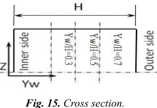
As illustrated in Fig. 11, the curved duct considered for the current calculation has a square cross section and a bend radius to duct height ratio of
Fig. 11. Curved duct.
2.3
=
R
H (10)
In order to obtain a fully developed parabolic velocity distribution before flow enters the bend, the upstream length of the duct is set to 20H. On the other hand, the downstream length of the duct is set to 26H to ensure a satisfied boundary condition at the outlet of the duct for carrying out the numerical calculations. With a Reynolds number of 40,000, a turbulence boundary condition is con-sidered in the case of the curved duct.
A grid–independent study was conducted, and the mesh was fixed to 50 × 50 for the square cross section, resulting in a total grid number of 433,664.
Fig. 12. Section of the grid of the curved duct.
By following the aforementioned methods for calculat-ing convective velocity, both the solvers delivered solu-tions for the flow field in the curved duct using the stan-dard k–ε turbulence model. After assessing the velocity fluctuation at a pre-defined point (monitor point), which is shown in Fig. 11, computational convergence procedures for both the solvers were carried out, and the results are compared in Fig. 13.
Fig. 13. Velocity oscillation in numerical calculation.
solver. This can be explained by the numerical stability analysis carried out in [3]. A stable Peclet number calcu-lated by the Sohrab solver dampens the numerical oscilla-tion and allows the calculaoscilla-tion to produce soluoscilla-tions that converge at a high speed. However, the two solvers pro-duce different velocities when convergence of their solu-tions is achieved. In the following figures, this difference in the velocities will be compared to the measurement data.
Fig. 14 shows a comparison of the computation time taken by the two solvers. The Navier–Stokes solver is twice slower than the Sohrab solver in completing the si-mulation. This result coincides with the analysis discussed above and shows the linear advantage of the Sohrab solver to solve a 3D flow problem.
Fig. 14. Comparison of computation time taken by both solvers.
In order to study the development of secondary flow mo-tion, the stream–wise and cross–wise velocities are com-pared at two locations: inside the bend (at θ = 60°) and downstream the bend (at Y = 0.25H), with different Yw positions, as shown in Fig. 15.
Fig. 15. Cross section.
Inside the bend of the duct, the fluid experiences a large curvature change and begins to follow a pressure-driven secondary flow motion. Therefore, at this location, the sec-ondary flow effect is marginal even though uniform veloci-ty distribution can still be observed.
Fig. 16. Comparison of the cross–wise and stream–wise velocity profiles inside the bend at θ = 60°.
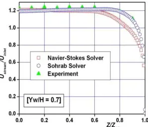
Downstream the bend at Y = 0.25H, the secondary flow feature continues to develop and the resultant variation in the compared with the measured data [9]. For stream–wise velocity profiles, it can be confirmed that both the solvers can predict secondary flow development very well. How-ever, in the cross–wise direction, the Navier–Stokes solver shows a very high velocity variation, particularly near the wall of the duct. This observation proves that the strength of the secondary flow calculated by the Naiver–Stokes solver is greater than the measured strength of the second-ary flow. In the case of the Sohrab solver, the secondsecond-ary flow calculated near the wall sufficiently agrees with the measured data, whereas the secondary flow calculated near the symmetry plane is observed to be low. Taking all the velocity profiles at this location into account, the Sohrab solver, as compared the Navier–Stokes solver, produces better results for the flow downstream the bend.
Fig. 17. Comparison of the cross–wise and stream–wise velocity profiles
downstream the bend at Y = 0.25H.
boundary layer case in [3] where in weak pressure–velocity coupling is observed; in both the cases, the Sohrab solver shows a linear advantage in carrying out the numerical calculations and consumes less computation resources.
4. Conclusions
In summary, a novel solver developed on the basis of the modified equation of fluid motion for incompressible flow is examined for different flow models, including models for laminar and turbulent flows. The solutions are validated by experimental data and numerical results obtained by calculating the classical Navier–Stokes equations. All the comparisons confirmed that the solutions obtained by the Sohrab solver are physically valid. The computational pro-cedure for the Sohrab solver was compared with that for the Navier–Stokes solver, and it was found that the former delivers a more efficient solution in terms of the linearity of the modified equation of fluid motion. This comparison demonstrates the scientific credibility of this novel solver for application to engineering flow problems. Further, we believe that if it is extended to design processes in the tur-bomachinery industry, significant improvements in the design cycle cost and time can be achieved.
Because of the encouraging results obtained in the cur-rent investigation carried out on fluid dynamic problems, the novel numerical solver further evidences the use of the finite-volume method to solve the modified equations of fluid motion.
Acknowledgment
The authors are very grateful to Prof. Siavash Sohrab, Northwestern University, IL. for his support and contribu-tion to this paper through helpful discussions.
Nomenclature
Cd
c
Drag coefficient Chord
D* Dimensionless distance (distance/boundary
layer length)
Fd Drag force
H Duct height
l Span
p* Dimensionless pressure (p/pmax)
p Pressure
R Bend radius
Re Reynolds number
t U*
Time
Dimensionless velocity (U/Umax)
Ue U uτ
Free stream velocity
Element velocity, local velocity Rate of shearing stress
u Atom velocity
v’ Peculiar velocity
w X, Y, Z Yw
Convective velocity Cartesian coordiantes Distance from the concave wall
Greek symbols
α Angle of attack
β Scale
δ Boundary layer thickness
ε Potential energy
θ Angle
ν Kinematic viscosity
ρ Density
Abbreviations
CFD Computational fluid dynamics
FVM Finite volume method
OpenFOAM Open field operation and manipulation
References
[1] Sohrab, S. H., “A Scale-Invariant Model of Statistical Me-chanics and Modified Forms of the First and the Second Laws of Thermodynamics”, International Journal of Ther-mal Science, vol. 38, pp. 845-853, 1999.
[2] Sohrab, S. H., 2008, “Derivation of invariant forms of con-servation equation from the invariant Boltzmann equation”, Proc 5th WSEAS Int. Conf. on Fluid Mechanics, S. H. So-hrab et al., eds, WSEAS Press, Athens, pp. 183-191.
[3] Wan, B., Benra, F.-K., and Dohmen, H. J., “Unique Numer-ical Scheme for a Modified Equation of Fluid Motion: Ap-proaching New Solver Development to a Fundamental Flow Problem”, Science Journal of Physics, vol. 2013, Article ID sjp-231, 2013.
[4] Sohrab, S. H., 2008, “A Modified Scale Invariant Statistical Theory of Turbulence,” Proc 6th WSEAS Int. Conf. on Flu-id Mechanics, S. H. Sohrab et al., eds, WSEAS Press, Athens, pp. 165-172.
[5] Thom, A., and Swart, P., “The forces on an aerofoil at very low speeds”, Journal of the Royal Aeronautical Society, vol. 44, pp. 761-770, 1940.
[6] Abbott, I. H., and von Doenhoff, A. E., “Theory of Wing Sections, including a Summary of Airfoil Data”, Dover Pub-lication, New York, pp. 165-169, 1959.
[8] Schultz-Grunow, F, “New Frictional Resistance law for Smooth Plates”, Luftfahrtforschung, vol. 17, pp. 239-246, 1940.
[9] Taylor, A. M. K. P., Whitelaw, J. H., and Yianneskis, M.,