SPC and Order Statistics: Burr Type XII Model

(1)

SPC and Order Statistics: Burr Type XII Model

Dr.R.Satya Prasad1, M.Anuradha2, Dr.G.Sridevi3 1

Assoc.Professor, Acharya Nagarjuna University, Guntur, India

2

Research Scholar, Acharya Nagarjuna University, Guntur, India

3

Professor, Malla Reddy Institute of Technology, Secunderabad, India.

Abstract — This paper presents a simple SRGM, the

Burr Type XII Non Homogeneous Poisson Process (NHPP) model is used as a control mechanism based on order statistics of the cumulative quantity between observations of time domain failure data. This model has the ability of modeling both reliability improving and deteriorating systems and has gained wide acceptance. The Maximum Likelihood Estimation (MLE) method is used to derive the point estimators. We have applied the model to sets of existing software failure datasets to assess the failure process using SPC.

Keywords — Burr type XII model, NHPP, MLE, Statistical Process Control, Order Statistics.

I. INTRODUCTION

Modern society relies heavily on the correct operation of software and from user„s point of view, the software plays an important role in systems of both safety-critical and civil applications. Software Reliability plays an important role in software quality. As more and more software is creeping into the embedded system, reliability has become an essential characteristic for the software. There are many software reliability models that are based on the times of occurrences of errors in debugging of the software. It is also possible to do asymptotic likelihood inference for software reliability models based on order statistics or Non – Homogeneous Poisson Processes (NHPP) with asymptotic confidence levels for interval estimates of parameters. In particular, interval estimates from these models are obtained for the conditional failure rate of the software, given the data from the debugging process. The data can be either grouped or ungrouped.

Software Reliability can prevent major faults that have the possibility of taking human life, money and time. For this a number of models have been developed for better predictions. A common

approach for measuring software reliability is by using an analytical model whose parameters are generally estimated from available software failure data. Reliability quantities have been defined with respect to time, although it is possible to define them

with respect to other variables. In reliability study there are two characteristics of a random process: 1) the probability distribution of the random variables, i.e., Poisson and 2) the variation of the process with time. A random process whose probability distribution varies with time is called non homogeneous. The random process for time variation we can define two functions, the mean value function m(t), as the average cumulative failures associated with each time point and the failure intensity function as the rate of change of mean value function.

Order statistics are used in a wide variety of practical situations. Their use in characterization problems, detection of outliers, linear estimation, study of system reliability, life-testing, survival analysis, data compression and many other fields can be seen from the many books example [1][2].

This paper presents a control mechanism is proposed which is based on the order statistics of cumulative quantity between observations of time domain failure data using mean value function of Burr Type XII distribution which is based on NHPP. The Burr Type XII distribution model with order statistics approach is applied on live data sets and the results are exhibited at the end of this paper.

II. ORDER STATISTICS

(2)

We compute the software failures process through Failure control chart based on the cumulative inter failure data. The transformation being applied is, the failure data is made into groups of 4, 5 and then cumulated. The inter failure time data represent the time laps between every two consecutive failures. On the other hand if a reasonable waiting time for failures is not a serious problem we can group the inter failure time data into non overlapping successive subgroups of size 4 or 5 and add the failures times with needs of groups. For instance if a data of 100 inter failure times are available, we can group them into 20 disjoint subgroups of size 5. The sum totals in each subgroup would represent the time laps between every 5th failures. In the theory of statistics such a subtotal is defined as the 5th order statistics in a sample of size 5. In general for inter failure data of size „m‟ if „r‟ is any natural number less than m and preferably a factor of „m‟ we can expediently divide the data into „p‟ disjoint subgroups(p=m/r) and the cumulative total meets subgroup indicate the time between every rth failure.

The probability distribution of such a time laps would be better in the r th order statistic in a subgroup of size „r‟. This would be equal to the rth power of the distribution function of the original variable. The parameters of the mean value function with the revised distribution function would determine the control limits of a new control chart involving order statistics. Hence they need a separate study.

In the present paper we have taken r = 4, 5 and the Burr Type XII model. Choice of r beyond 5 may create an overly long waiting time for the occurrence of every rth failure. „a‟,‟b‟ and „c‟ are Maximum Likelyhood Estimates (MLEs) of parameters and the values can be calculated using iterative method for the given cumulative time between failures data. Using „a‟ and „b‟ and „c‟ values we can compute m(t).

III. IIUSTRATING THE MLE

METHOD

Burr Type XII Model

This paper proposes estimation of software reliability using order statistics approach based on Burr Type XII distribution model. The Burr distribution has a flexible shape and controllable scale and location which makes it appealing to fit to data. It is frequently used to model insurance claim sizes. The mean value function and intensity function of Burr Type XII NHPP model are as follows [8][15].

The Cumulative distributive function (CDF) is given by





1

0

( )

1

c b

m t





t dt



a



_

 

t





_







(1)



a F t

( )

The Probability Density Function (PDF) of Burr XII distribution are given, respectively by





1

( )

1

c

b c

cbt

t

a

a f t

t



 













_







Mathematical Derivation for Parameter Estimation

We develop expressions to estimate the parameters of the Burr type XII model based on time domain data using order statistics approach. Parameter estimation is very significant in software reliability prediction. Once the analytical solution form is known for a given model, parameter estimation is achieved by applying a well-known estimation, Maximum Likelihood Estimation (MLE).

The main idea behind Maximum Likelihood parameter assessment is to decide the parameters that maximize the probability (likelihood) of the specimen data. In other words, MLE methods are versatile and applicable to most models and for different types of data.

The mean value function of Burr type XII model is given by [8]





( )

1

c b

,

0 m t



a



_

 

t





_

t







(1)

The parameters a, b, c are estimated with Maximum Likelihood (ML) estimation. In order to group the Time domain data into non overlapping successive sub groups of size r, we need to take m t( ) to the power r.









( ) 1 1

r b c

m t _a  t  _

 

(2)

(3)

( ) 1

'( )

n m t i i

L

e



m t





(3)









1 1 1 (1 )

1

r c b r c n a t b b c c i

a

abct

L

e

r a

t

      _  _  















_



_



















1 1 1 1 1 1

log ( 1) log 1

log log log ( 1) log ( 1) log( 1)

r r b c n n b c i i i n c i i i L a t a

Log r r a

t

a b c c t b t

            _ _     _  _      _ _       



Differentiating Log L with respect to „a‟, and

equating to 0 (i.e., LogL 0

a

 

 ) we get









1

r b c r b c

t

a

n

t



_











_

_







(4)

Differentiating Log L with respect to „b‟ and equating

to „0‟. 0 LogL b  _    1 1

1 1 1

( ) log log log( 1)

( 1) 1 1 1 1 1

n n

i b

b

i i i i

nr r n

g b t

t t  t t b 

          _ _  _ _ _ _ _ _  _ _            (5) Again differentiating g b( ) with respect to „b‟ and

equating to 0

2

. ., LogL 0

i e b      _               

2 2 2

1

1 log 1 1 log 1

1 1

'( ) log log

1 ₁ ₁ 1 ₁ ₁

b _n b

i i

b b

i i

i

t t t t n

g b nr

t _t  t _t b

          _ _  _ _      _   _



  _   _ (6)

Differentiating Log L with respect to „c‟ and equating

to „0‟. 0 LogL c   





1  1

log

log 2

( ) 1 log .log

1 1

1

n n

c i

i i i

c c

c

i i i i

t

t n

g c nr r t t t

t c t

t  

        _    _     _          



(7) Again differentiating ( )g b with respect to „b‟ and

equating to 0

2

. ., LogL 0

i e c   _   _     





_

_

2 2 2 2 1 1

'( ) 2 log . (1 )

1 2 log . 1

log 2 log log 1 1 c c c i n n

i _c c

i i i i

i c

i i

i

t

g c nr t

t

t n

r t

t t t t

c t t      _ _      _ _    _ _ _ _ _ __    _ _  _ __   _ _ _    



(8) The parameters „b‟ and „c‟ are estimated by iterative Newton- Raphson using

1

( )

'( )

n n n n

g b

b

g b



 

1

( )

'( )

n n n n

g c

c

g c



 

Which are substituted in Eq.(4) to determine „a‟.

Estimated Parameters and their Control Limits

[9] estimated the parameters using maximum likelihood estimation using interfailure time data. The control limits for the chart are defined in such a manner that the process is considered to be out of control when the time to observe exactly one failure is less than LCL or greater than UCL. Our aim is to monitor the failure process and detect any change of the intensity parameter.

When the process is normal, there is a chance for this to happen and it is commonly known as false alarm. The traditional false alarm probability is to set to be 0.27% although any other false alarm probability can be used [12]. The actual acceptable false alarm probability should in fact depend on the actual product or process [13].

(4)

( )c

m t and LCL= m t( )l . They are used to find

whether the software process is in control or not. The estimated values of „a‟ and „b‟ and „c‟ and their control limits for both 4th -order and 5th -order statistics are as follows.

Calculation of control limits

0.99865 0.5 0.00135

u

c

l

T T T

  

Table 1: Parameter estimates and Control limits of 4 & 5 order

Data Set Order

Estimated Parameters Control Limits

a b c UCL CL LCL

Musa 4 8.50 0.927761 1.000346 8.488525 4.250000 0.011471

5 5.40 0.939095 1.000277 5.392710 2.700000 0.007289

Sys 2 4 5.25 0.901900 1.000173 5.242913 2.624999 0.007089

5 3.40 0.919045 1.000135 3.395410 1.6999999 0.004589

Distribution of Time between Failures

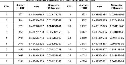
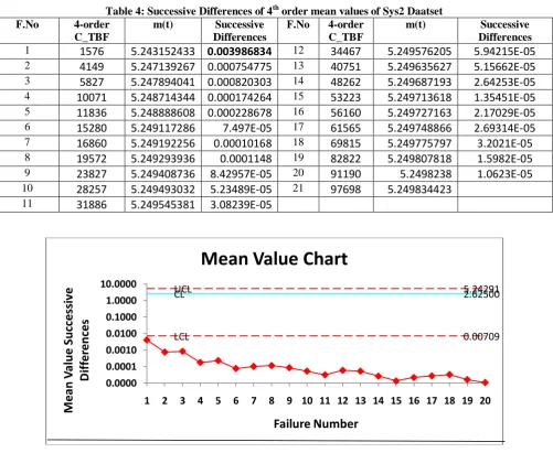
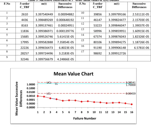
The mean value successive differences of rth order cumulative time between failures data of the considered data sets are tabulated in Table 2 to 5. Considering the mean value successive differences on y axis, failure numbers on x axis and the control limits on Failure control chart, we obtained Figure 1

to 4. A point below the control limit m t( )_l indicates an alarming signal. A point above the control limit

( )u

m t indicates better quality. If the points are falling within the control limits it indicates the software process is in stable.

Table 2: Successive Differences of 4th order mean values of Musa F.No 4-order

C_TBF m(t)

Successive

Differences F.No

4-order

C_TBF m(t)

Successive Differences

1 227 8.444910865 0.025473171 18 16358 8.498955984 0.000102605

2 444 8.470384036 0.011594542 19 18287 8.499058589 9.72543E-05

3 759 8.481978577 0.004752661 20 20567 8.499155843 0.000116243

4 1056 8.486731238 0.005882555 21 24127 8.499272086 0.000103446

5 1986 8.492613794 0.001785012 22 28460 8.499375533 7.09241E-05

6 2676 8.494398806 0.002095267 23 32408 8.499446457 7.19499E-05

7 4434 8.496494073 0.000420743 24 37654 8.499518407 4.65714E-05

8 5089 8.496914816 0.000159693 25 42015 8.499564978 2.68286E-06

(5)

10 6380 8.497498674 0.000334377 27 48296 8.499617742 2.56036E-05

11 7447 8.497833051 0.000120836 28 52042 8.499643345 8.68534E-06

12 7922 8.497953886 0.000436267 29 53443 8.499652031 1.74262E-05

13 10258 8.498390153 0.000122963 30 56485 8.499669457 3.03022E-05

14 11175 8.498513115 0.000152686 31 62651 8.499699759 9.63903E-06

15 12559 8.498665801 8.53239E-05 32 64893 8.499709398 3.98085E-05

16 13486 8.498751125 0.000136472 33 76057 8.499749207 3.33167E-05

17 15277 8.498887597 6.8387E-05 34 88683 8.499782523

Fig 1: Failure Control Chart for Musa Dataset of order 4

Table 3: Successive Differences of 5th order mean values of Musa Dataset

F.No 5-order

C_TBF

m(t) Successive Differences

F.No 5-order C_TBF

m(t) Successive

Differences

1 ₃₄₂ _{5.377568698 0.008556681} 15 ₁₇₇₅₈ _5.399449597 _7.09183E-05

2 ₅₇₁ _5.38612538 _0.005418403 16 ₂₀₅₆₇ _5.399520515 _9.35047E-05

3 ₉₆₈ _{5.391543783 0.004148817} 17 ₂₅₉₁₀ _5.39961402 _4.27728E-05

4 ₁₉₈₆ _{5.3956926 0.001470152} 18 ₂₉₃₆₁ _5.399656793 _7.14374E-05

5 ₃₀₉₈ _{5.397162753 0.001043802} 19 ₃₇₆₄₂ _5.39972823 _2.66574E-05

6 ₅₀₄₉ _{5.398206554 8.71412E-05} 20 ₄₂₀₁₅ _5.399754887 _1.72349E-05

7 ₅₃₂₄ _5.398293696 _0.00026667 21 ₄₅₄₀₆ _5.399772122 _1.7414E-05

8 ₆₃₈₀ _{5.398560366 0.000224782} 22 ₄₉₄₁₆ _5.399789536 _1.45114E-05

9 ₇₆₄₄ _{5.398785148 0.000278761} 23 ₅₃₃₂₁ _5.399804048 _1.03283E-05

10 ₁₀₀₈₉ _5.399063909 _7.1677E-05 24 ₅₆₄₈₅ _5.399814376 _1.72389E-05

11 ₁₀₉₈₂ _{5.399135586 0.000102358} 25 ₆₂₆₆₁ _5.399831615 _2.50181E-05

12 ₁₂₅₅₉ _{5.399237944 0.000105074} 26 ₇₄₃₆₄ _5.399856633 _1.63088E-05

13 ₁₄₇₀₈ _{5.399343018 5.64761E-05} 27 ₈₄₅₆₆ _5.399872942

14 ₁₆₁₈₅ _{5.399399494 5.01026E-05}

UCL=8.48853

CL=4.25000

LCL=0.01147

0.0000 0.0000 0.0001 0.0010 0.0100 0.1000 1.0000

1 3 5 7 9 11 13 15 17 19 21 23 25 27 29 31 33

M

e

an

V

al

u

e

S

u

cc

e

ssi

ve

D

if

fe

re

nc

es

Failure Number

(6)

Fig 2: Failure Control Chart for Musa Dataset of order 5

Table 4: Successive Differences of 4th order mean values of Sys2 Daatset

F.No 4-order

C_TBF

Differences

1 ₁₅₇₆ _5.243152433 _0.003986834 12 ₃₄₄₆₇ _5.249576205 _5.94215E-05

2 ₄₁₄₉ _{5.247139267 0.000754775} 13 ₄₀₇₅₁ _5.249635627 _5.15662E-05

3 ₅₈₂₇ _{5.247894041 0.000820303} 14 ₄₈₂₆₂ _5.249687193 _2.64253E-05

4 ₁₀₀₇₁ _{5.248714344 0.000174264} 15 ₅₃₂₂₃ _5.249713618 _1.35451E-05

5 ₁₁₈₃₆ _{5.248888608 0.000228678} 16 ₅₆₁₆₀ _5.249727163 _2.17029E-05

6 ₁₅₂₈₀ _5.249117286 _7.497E-05 17 ₆₁₅₆₅ _5.249748866 _2.69314E-05

7 ₁₆₈₆₀ _5.249192256 _0.00010168 18 ₆₉₈₁₅ _5.249775797 _3.2021E-05

8 ₁₉₅₇₂ _5.249293936 _0.0001148 19 ₈₂₈₂₂ _5.249807818 _1.5982E-05

9 ₂₃₈₂₇ _{5.249408736 8.42957E-05} 20 ₉₁₁₉₀ _5.2498238 _1.0623E-05

10 ₂₈₂₅₇ _{5.249493032 5.23489E-05} 21 ₉₇₆₉₈ _5.249834423

11 ₃₁₈₈₆ _{5.249545381 3.08239E-05}

Fig 3: Failure Control Chart for Sys2 Dataset of order 4

UCL=5.39271

CL=2.70000

LCL 0.00729

0.0000 0.0001 0.0010 0.0100 0.1000 1.0000 10.0000

1 2 3 4 5 6 7 8 9 10 11 12 13 14 15 16 17 18 19 20 21 22 23 24 25 26

M

e

an

V

al

u

e

S

u

cc

e

ssi

ve

D

if

fe

re

n

ces

Failure Number

Mean Value Chart

UCL 5.24291

CL 2.62500

LCL 0.00709

0.0000 0.0001 0.0010 0.0100 0.1000 1.0000 10.0000

1 2 3 4 5 6 7 8 9 10 11 12 13 14 15 16 17 18 19 20

M

e

an

V

al

u

e

S

u

cc

e

ssi

ve

D

if

fe

re

n

ces

Failure Number

(7)

Differences

1 ₂₆₁₀ _3.397540449 _0.00094882 10 ₃₉₈₅₆ _3.399799166 _2.53111E-05

2

4436 3.398489269 0.000648192 11 46147 3.399824477 2.15703E-05

3

8163 3.399137461 0.00024951 12 53223 3.399846047 1.39037E-05

4

11836 3.399386971 0.000139776 13 58996 3.399859951 1.60915E-05

5

15685 3.399526746 5.61415E-05 14 67374 3.399876043 1.82326E-05

6

17995 3.399582888 7.35854E-05 15 80106 3.399894275 1.18726E-05

7

22226 3.399656473 6.8023E-05 16 91190 3.399906148 6.5781E-06

8

28257 3.399724496 3.2183E-05 17 98692 3.399912726

9

32346 3.399756679 4.24866E-05

Fig 4: Failure Control Chart for Sys2 Dataset of order 5

IV. CONCLUSIONS

The 4 and 5 order failure counts are plotted through the estimated mean value function against the rth failure (i.e 4 & 5) serial order. The MLE method is used to estimate the parameters. The successive differences of the Musa dataset are fairly fluctuating within the control limits and the successive differences of Sys2 dataset have gone out of control limits. Hence we conclude that our method of estimation and the control chart are giving a Positive recommendation for their use in finding out preferable control process or desirable out of control signal.

REFERENCES

[1] Balakrishnan. N., Clifford Cohen. A., (1991), “Order Statistics: Theory and Methods, Hand Book of Statistics”, Vol. 16, Elsevier.

[2] Arak M Mathai, (2003), “On the distribution of order statistics from generalized logistic samples”.

[3] Crow. L. H. (1974). “Reliability for Complex Systems, Reliability and Biometry”, Society for Industrial and

[4] Duane, J.T., (1964). “Learning curve approach to reliability monitoring”, IEEE Trans. Aerospace, AS-2, pp.[563-566].

[5] M. Horigome, N. D. Singpurwalla, and R. Soyer. (1984). “A Bayes Empirical Bayes Approach for Software Reliability growth”. In Computer Science and Statistics, (16th Symp. Interface, Atlanta, GA), NorthHolland, pp.47-55.

[6] Khoshgoftaar, T.M. and Woodstock, T.G. (1991). “Software reliability model selection: a case study”, Proc. Int. Symp. On software reliability engineering, may 18-19, Austin, Texas, pp.[183-191].

[7] Lyu, M.R. and Nikora, A. (1991). “A Heuristic approach for software reliability prediction: the equally weighted linear combination model. Proc. Int. Symp. On software reliability engineering, may 18-19, Austin, Texas, pp.[172-181].

[8] Gutta Sridevi, R.Satya Prasad and K.V.Murali Mohan, “Monitoring Burr Type XII Software Quality Using SPC”,International Journal of Applied Engineering Research (IJAER), Vol. 9, No. 22 (2014), pp:16651-16660, ISSN:0973-4562.

[9] Xie, M and Zhao, M, “On some reliability growth models with simple graphical interpretations”, to appear in Microelectronics and reliability.

[10] Lyu, M. R., (1996). “Handbook of Software Reliability Engineering”. McGraw-Hill publishing, ISBN 0-07-039400-8.

UCL _CL 3.39541 1.70000

LCL 0.00459

0.0000 0.0000 0.0001 0.0010 0.0100 0.1000 1.0000

1 2 3 4 5 6 7 8 9 10 11 12 13 14 15 16

M

e

an

V

al

u

e

S

u

cc

e

ssi

ve

D

if

fe

re

nc

es

Failure Number

(8)

[12] Xie. M, T.N Goh and P.Ranjan. (2002). “Some effective control chart procedures for reliability monitoring”, Reliability Engineering and System Safety. 77, 143-150. [13] Gokhale, S.S and Trivedi, K.S., 1998. “Log-Logistic

Software Reliability Growth Model”. The 3rd IEEE International Symposium on HighAssurance Systems Engineering. IEEE Computer Society.

[14] Lyu, M. R., (1996). “Handbook of Software Reliability Engineering”. McGraw-Hill publishing, ISBN 0-07-039400-8.

[15] Burr (1942), “Cumulative Frequency Functions”, Analysis of Mathematical Statistics, 13, pp. 215-232.