MONITORING CHANGE IN LAKE WATER STORAGE OVER TIME WITH SATELLITE IMAGERY AND CITIZEN SCIENCE
Sarina Anne Basile Little
A thesis submitted to the faculty at the University of North Carolina at Chapel Hill in partial fulfillment of the requirements for the degree of Master of Science in the Department of
Geology.
Chapel Hill 2020
© 2020
ABSTRACT
Sarina Anne Basile Little: Monitoring change in lake water storage over time with satellite imagery and citizen science
(Under the direction of Tamlin Pavelsky)
Despite lakes being key part of the global water cycle and a crucial water resource, there is limited understanding of how water storage in small lakes varies over time. Here, we study change in lake water storage over time in clusters of small natural lakes in North Carolina, Washington, Illinois, and Wisconsin, using lake level measurements gathered by citizen
ACKNOWLEDGEMENTS
TABLE OF CONTENTS
LIST OF FIGURES………vii
LIST OF TABLES………... viii
LIST OF ABBREVIATIONS……… ix
1. Introduction……….…………... 1
2. Background Information……….………… 5
2.1 Citizen Science in Surface Water Hydrology..………..……….……… 5
2.2 Lake Area from Optical Satellite Imagery…………..……… 7
2.3 Monitoring Lake Water Storage Using Satellites……….………. 10
3. Study Area………...………. 13
3.1 North Carolina………..……… 13
3.2 Washington………...……… 14
3.3 Illinois………...……… 14
3.4 Wisconsin………..………... 15
4. Methods………...………. 15
4.1 Measuring Lake Water Levels……….………. 16
4.1.1 Data Acquisition………. 16
4.1.2 GPS Processing………... 17
4.1.3 Validation………...……… 19
4.2 Measuring Lake Surface Area………...……… 19
4.2.2 Water Mask………...………...………...……… 20
4.2.3 Validation………...……… 21
4.3 Measuring Lake Water Storage……….……… 22
4.3.1 Calculation of Lake Water Storage……….……… 23
4.3.2 Rating Curve………...……… 24
4.3.3 Validation………...……… 24
4.4 Correlations between Change in Lake Water Storage………...… 25
4.4.1 Calculating Correlations……….……… 25
4.4.2 Validation………...……… 25
4.5 Spatial Analysis……… 26
5. Results………... 26
5.1 Validation Results……….……… 26
5.1.1 Citizen Science Data………...……… 26
5.1.2 Lake Surface Area………...……… 26
5.1.3 Lake Volume Correlations………..………… 27
5.2 Variations in Lake Water Storage……….……… 27
5.2.1 Correlation between the Change in Lake Water Volume……… 27
5.2.2 Correlations and Relationship with Distance………..……… 28
6. Discussion………. 28
FIGURES………..……… 33
TABLES……… 49
APPENDIX: SUPPLEMENTAL INFORMATION……….……… 50
LIST OF FIGURES
Figure 1. Lake gauge locations ……….………...…. 33
Figure 2. A LOCSS lake gauge ……… …….……….. 34
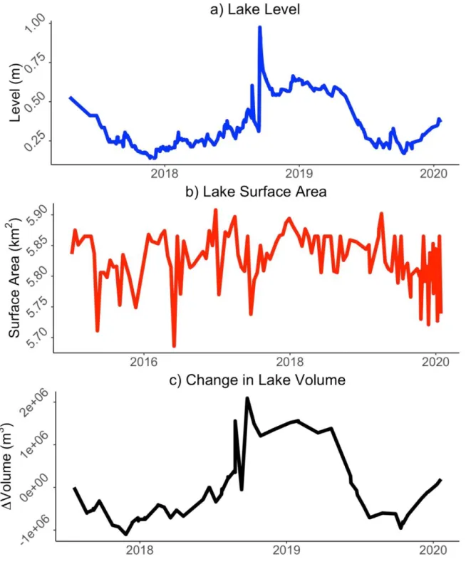
Figure 3. Lake level, surface area, and change in lake volume in Bay Tree Lake…...…..…….... 35
Figure 4. Lake water surface extent classifications……….……….. 36
Figure 5. Planet imagery lake surface extent……….……….... 37
Figure 6. Rating curve linear relationship………...…….……….. 38
Figure 7. Change in lake water volume over time from rating curve………….……….………. 39
Figure 8. Change in lake water volume at Grays Lake (citizen science and pressure transducer data)………...………..………..… 40
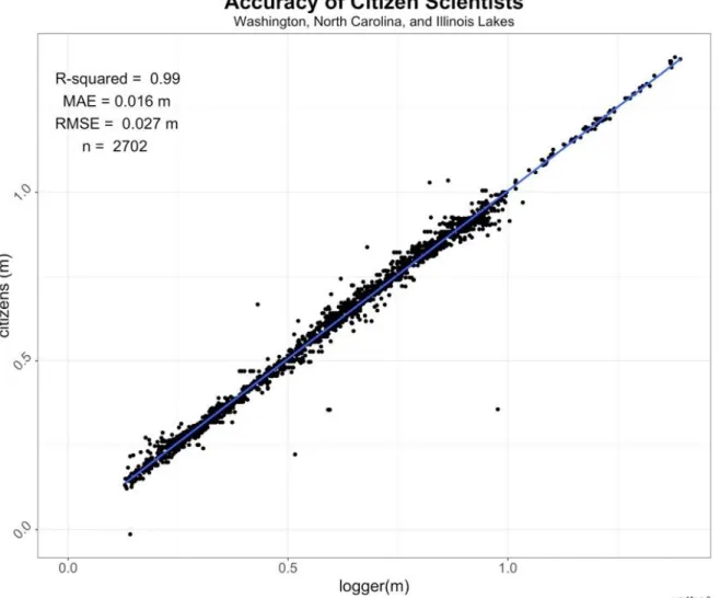
Figure 9. Accuracy of citizen science data………. 41
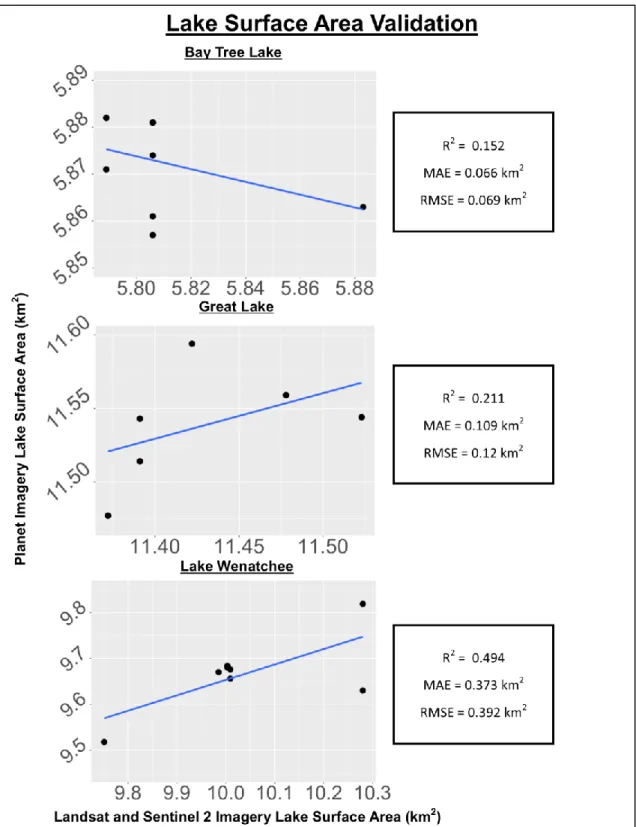
Figure 10. Lake surface area validation………. 42
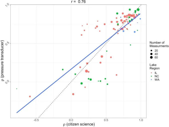
Figure 11. Correlation coefficient validation………. 43
Figure 12. Distribution of correlation coefficients ……… 44
Figure 13. Examples of high, moderate, and low correlations ………..… 45
Figure 14. Relationships between and distance…………..……… 46
Figure 15. Relationships between and number of measurements .…….……… 47
LIST OF TABLES
LIST OF ABBREVIATIONS DNR Department of Natural Resources
DSWE Dynamic Surface Water Extent G3WBM Global 3 arc-second Water Body Map GEE Google Earth Engine
GFO Geosat Follow On
LOCSS Lake Observations by Citizen Scientists and Satellites MAE Mean Absolute Error
MODIS Moderate Resolution Imaging Spectroradiometer MSS Multispectral Scanning Systems
NHD National Hydrography Dataset RMSE Root Mean Square Error SAR Synthetic-aperture radar SWO Surface Water Occurrence
MONITORING CHANGE IN LAKE WATER STORAGE OVER TIME WITH SATELLITE IMAGERY AND CITIZEN SCIENCE
1. Introduction
Surface water stored in lakes is a key part of the global water cycle and a crucial water resource, providing drinking water, supporting irrigation systems, promoting economic activity and tourism, and generating hydroelectric power. In addition to supporting human activities, lakes sustain diverse natural biological, chemical, and physical systems important for many natural processes. Lakes encompass geographically diverse areas, are the lowest points in their surrounding landscapes, serve as records of past hydrologic and geologic events, and regulate surrounding climate. Because they integrate so many processes, lakes and reservoirs act as sentinels of climate change and are amongst the most threatened by climate change and other human impacts (MEA 2005; Adrian et al., 2009; Williamson et al., 2009; IPCC 2014). Lake water level, especially in endorheic lakes, is very sensitive to changes in the water balance (Williamson et al., 2009; Wang et al., 2018). Studying ongoing changes in lakes allows us to better understand the effects climate change on the water cycle and better predict the future of lake systems in the context of global climate change (Adrian et al., 2009; Williamson et al., 2009).
2013; Song et al., 2013; Khadka et al., 2018; Li et al., 2019), precipitation, and regional human activities, such as mining (Li et al., 2019). Numerous lakes in the Mediterranean climate zone are experiencing decreases in water level, increases in eutrophication, and increased salinity due to changes in climate and irrigation (Jeppesen et al., 2014). While remaining stable over the last two decades (Pham-Duc et al., 2020), Lake Chad, in northwest Africa, experienced a 90% decline in lake area by the end of the 1980s (Leblanc et al., 2011) due to prolonged drought and an increase in irrigation of farmland (Coe & Foley, 2001); it is now divided into a series of seasonal and perennial lakes with high variability and vulnerability (Lemoalle et al., 2012). The Aral Sea, among the greatest human-driven disasters of recent decades, has decreased by 23 meters in lake level, 74% in area, and 90% in volume while increasing in salinity tenfold (Micklin, 2006). What was once one sea has now desiccated into three small waterbodies, each of which acquiring very different hydrologic features (Izhitskiy et al., 2016).
Measurement networks, however, whether in situ or satellite-based, tend to focus mostly on larger lakes, with general oversight of small lentic water bodies. Lakes smaller than 10 km2 are generally poorly observed and monitored. There are, however, many more small lakes than large lakes. Of the 300 million lakes with a surface area greater than 0.001 km2 (Verpoorter et al., 2014), about 136 million have a surface area between 0.002 and 0.01 km2 (Downing et al., 2006). Combined, their surface area is an estimated 272,000 km2 – 1,360,000 km2. The total surface area of lakes increases with decreasing water body size (Downing et al., 2006; Verpoorter et al., 2014; Messager et al., 2016), demonstrating that most of the global
While there have been studies looking at regional patterns of change in lake water level (Euliss & Mushet, 1996; Watras et al., 2014) or surface area (Cooley et al., 2019) and while many ecologists do study small lake ecosystems, variations in lake water storage remains poorly constrained in current hydrology research despite their abundance and hydrological significance. A handful of studies (e.g. Lei et al., 2013; Zhang et al., 2017; Qiao et al., 2019), mostly focused on the Tibetan Plateau, that have studied controls on lake volume across multiple lakes within a region. However, our understanding remains limited regarding how the storage of water in small lakes fluctuates, how they differ from large lakes in terms of these fluctuations, what controls these fluctuations, and the implication of these fluctuations on the ecosystem services they provide (Hanson et al., 2007; Downing, 2009).
This gap in knowledge regarding small lakes is in large part caused by limitations in current lake monitoring systems. Because lake systems are such important sentinels of environmental change, there is an increased need for the development of local, regional, and global scale networks that collect data on lakes (Williamson et al., 2009). To date, lake monitoring is primarily done through government-run gauge networks, studies by individual scientists, and satellite radar altimetry. In the United States, the largest gauge network is maintained by the United States Geological Survey (USGS) and includes around 300 lakes. While the USGS monitors fluctuations in water levels in rivers and lakes, most monitored lakes are man-made or dammed reservoirs, while only a handful are natural lakes. These are mostly relatively large in size. Many state and local governments have their own gauge networks, such as Lake Level Minnesota (DNR,
data, however, is often not widely shared, is spatially and temporally discontinuous, and is not in consistent formats. Similar problems exist for datasets collected by individual scientists. This leaves the majority of the natural lakes in the United States unmonitored. Similar deficiencies exist elsewhere in the world (Shiklomanov et al., 2002; IAHS, 2001; Stokstad, 1999).
Furthermore, there has been an overall decline in gauging networks due to a lack of funding, lack of personnel for installation and data collection, and difficulty of installation (Fekete et al., 2015). Satellite radar altimetry serves as a method for monitoring lake water level and lake water volume in areas where in situ measurements are not available, as well as provide
measurements over relatively long-time spans (Crétaux et al., 2016). These measurements, which are increasingly applicable to smaller lakes (Baup et al., 2014; Kleinherenbrink et al., 2020), remain most effective for lakes larger than 1-10 km2 (Arsen et al., 2015; Hughes, 2006) and are available only for a small fraction of lakes worldwide because satellite altimeter ground tracks are widely spaced (Alsdorf et al., 2007).
et al., 2014; Lowery et al., 2019; Strobl et al., 2019). By combining measurements of lake area from satellites and stage measured by citizen scientists, we can measure variations in lake volume, a key variable in understanding the water cycle and water resource availability. Using this water storage data, we can address key science questions in lake hydrology.
The objective of this research is to understand what factors control regional patterns of lake water storage. We test whether the storage of water in regional clusters of small lakes varies in concert, suggesting regional-scale drivers of the variation, or if such variations are primarily driven by local factors unique to each lake. To achieve this objective, we calculate change in lake water storage over time in clusters of small natural lakes in Wisconsin, Illinois, North Carolina, and Washington, USA through the use of lake level measurements gathered by citizen scientists and lake extent measurements taken from optical satellite imagery. We compare these time series of water storage between lakes within regional clusters. If time series within a cluster are highly correlated, then controls on lake water storage are likely regional in nature. If they are uncorrelated, then local controls specific to each lake must be relatively important.
2. Background
2.1 Citizen Science in Surface Water Hydrology
al., 2014; Minnesota Pollution Control Agency, 2014; US Environment Protection Agency, 2014; Koch and Stisen, 2017). Starting in the last decade, several projects have asked citizen scientists to provide information about water levels in rivers, lakes, and streams. For example, CrowdHydrology, a citizen science project that monitors water levels in rivers and some lakes through the use of gauge networks, simple instructional signage, and a text message data collection system, demonstrates that this is possible (Fienen and Lowry, 2012; Lowry and Fienen, 2012). In scaling up from a small regional project to a national scale project, the CrowdHydrology team has explored the difficulties and successes in establishing a hydrology citizen science network (Lowry et al., 2019). They suggest that it is possible to establish and scale up a citizen science network, that crowdsourced data collection is a viable method for gathering supplemental hydrologic data, and that citizen science projects are a promising method of public engagement for hydrologists. They further suggest that ongoing communication is critical for volunteer retention, that a relatively small group of core volunteers maintain the project, and that convenient gauge location is essential for success (Lowry and Fienen, 2012; Lowry et al., 2019).
The CrowdWater game takes a different approach to monitoring water levels (Strobl et al., 2019) by partnering with citizen scientists to add and quality check water levels through
photographs of riverbank structures. Strobl et al. explore the motivations of players, the success of image and lake level measurement quality checks, and how to retain long term users.
Retention is particularly important because experienced players produced higher quality observations (Strobl et al., 2019).
et al., 2014). For example, data collected by citizen scientists can provide validation for remote sensing results (Koch and Stisen, 2017). Although the accuracy of data collected by citizen scientists is one of the biggest concerns about the partnership with citizen scientists in scientific studies (Cohen 2008), recent studies suggest that, when trained and properly informed, citizen scientists can provide very accurate measurements (Cohen, 2008; Hunter et al., 2012; Buytaert et al., 2014). Two challenges that still arise with the use of citizen science networks, however, are sparse spatial and temporal sampling; it is difficult to recruit a network of citizen scientists over a large region, and it is difficult to find citizen scientists who take measurements on a regular basis.
2.2 Lake Area from Optical Satellite Imagery
Over the last four decades, numerous studies have demonstrated that lake water surface extent can be captured using optical satellite imagery (Gupta & Banerji, 1985; Kite & Pietroniro, 2000; Mueller et al., 2016; Huang et al., 2018; Ogilvie et al. 2018). Many studies specifically use Landsat imagery on a regional scale to study changes in lake water extent (Song et al., 2013; Mueller et al., 2016; Sheng et al., 2016; Tulbure et al., 2016; Avisse et al., 2017; Khadka et al., 2018; Ogilvie et al., 2018; Zhang et al., 2018). The Landsat 5 – 8 sensors, with a spatial
and their results suggested that the fixed-threshold modified normalized difference water index (MNDWI) is the most accurate when calculating lake surface area for small lakes, providing viable data for lakes as small as 0.01 km2. Accuracy decreases, however, for lakes smaller than 0.03 km2 using Landsat imagery alone. Using a combination of Landsat and Sentinel 2 imagery, however, Ogilvie et al. further reduce classification errors and increase the feasibility of
monitoring small water bodies. Overall, they suggest that ongoing technological improvements are increasing opportunities for remote sensing of surface area in small lakes (Ogilvie et al., 2018). Other regional studies have also examined the potential of remote sensing methods to observe surface water areas of small lakes, from 0.01 to 0.025 km2 (Liebe et al., 2005;
Sawunyama et al., 2006; Soti et al., 2006; Mialhe et al., 2008; Annor et al., 2009; Gardelle et al., 2010; Rodrigues et al., 2011; Jones et al., 2017), however problems of accuracy on lakes <1 km2 prevail (Annor et al., 2009; Ran & Lu, 2012; Solander et al., 2016).
constellation. This fine resolution imagery provides regular estimates of lake surface extent in small lakes (Cooley et al., 2017). With these new technologies, it is increasingly possible to track surface water extent variations for lakes smaller than 1 km2.
There are advances in data products that are also making it more possible to accurately detect waterbody extent. For example, Pekel et al. (2016) used Landsat imagery to study global surface water dynamics over a 30-year time period, including water bodies as small as one Landsat pixel. Similarly, the Global 3 arc-second Water Body Map (G3WBM) developed and described by Yamazaki et al. (2015) provides a useful accounting of water bodies globally. In addition to new sensors and data products, new methods of extracting inundation extent are increasingly making it possible to automate lake area detection globally. Jones (2019) from the USGS developed the “Dynamic Surface Water Extent” (DSWE) Landsat Science Product. This product improves classification of water pixels from Landsat imagery, especially in wetland areas, relative to other available products. The DSWE algorithm classifies pixels into five categories; high, moderate, or low probability of water, inundated vegetation, or not water. Errors do still occur in shadowed pixels, where thick mixed forest canopies are present, and where sun angles are low (Jones, 2019). The study was directed at detecting variations in inundation extent, however can be applied to variations in lake surface area dynamics. Additionally, DSWE has further been used with Sentinel 2 imagery after applying a
2.3 Monitoring Lake Water Storage Using Satellites
of some sensors, long revisit times (Baup et al., 2014; Avisse et al., 2017). Furthermore, satellite altimeters still require some in situ, ground-truthing, especially as new sensors are launched and new data processing methods are developed (Hughes, 2006; Calmant et al., 2008).
Satellite optical imagery provides another mechanism in which lake water volume can be calculate. As described in section 2.2, satellite optical imagery provides measurements of lake surface extent. When pairing these measurements with depth data, lake storage can be calculated. As mentioned in the previous paragraph, one way to calculate waterbody storage and change is through the use of satellite optical imagery and satellite radar altimetry, which has been widely used (Crétaux et al., 2016). For example, Kropáček et al., (2012) studied Lake Namco, located in the central Tibetan Plateau, using Landsat satellite imagery and Geosat Follow On (GFO), Envisat and ICEsat satellite altimetry data to model water budgets and total volume change.
Another way that waterbody storage has been estimated with optical satellite imagery is in being paired with topographic data. One early study, by Gupta & Banerji (1985), used Landsat multispectral scanning systems (MSS) along with topographic data to monitor fluctuations in water volume over time in the Ramganga dam reservoir in the Himalayas. Zhang et al. (2011) also estimated water storage changes in Lake Namco using Landsat satellite images and in situ water depth from lake bathymetry, rather than satellite altimetry. Lei et al. (2013) applied a similar analysis but included five other lakes in the Tibetan Plateau as well. Liebe et al., (2005) estimated lake water storage in the Upper East Region of Ghana using an area-volume
relationship, which allowed them to only use satellite imagery. They determined the relationship, however, by pairing lake surface extent calculated from Landsat imagery with lake bathymetry data. Sawunyama et al. (2019) applied a similar analysis on 12 small reservoirs in the
There have also been efforts to measure lake volume variations using in situ
measurements of stage and satellite measurements of area. Smith & Pavelsky (2009) used in situ stage measurements and MODIS satellite imagery to calculate change in lake water storage for nine lakes, ranging in size between 1.5 and 1,313.2 km2, in the Peace-Athabasca Delta in Canada. They noted the importance of accurate surface area and stage measurements to confidently measure change in lake water storage, as some lakes are more sensitive to area variations and others to stage. Similarly, Medina et al. (2010) made a first estimate of water volume variations in Lake Izabal, Guatemala by combining lake water levels monitored through in situ gauges in the lake and from the ENVISAT Radar Altimeter (RA-2) with lake surface extent measurements from ENVISAT Advanced Synthetic Aperture Radar (ASAR) images. They developed a rating curve between level, area, and volume to expand the volume variation data.
These studies are becoming more frequent and more accurate; however, they too have mostly been applied to large lakes. Lake volume studies have not been extensively conducted or validated for smaller lakes largely because the technologies for measuring area and surface water extent in small lakes are not as precise. Future satellites, such as the Surface Water and Ocean Topography (SWOT) satellite mission set to launch in 2022, will provide measurements of lake water level and surface area, as well as volume variations for lakes as small as 250 m by 250 m (Biancamaria et al., 2016; Grippa et al., 2019). For the first time, SWOT will provide
10 cm. Accuracies will decline with lake size (Biancamaria et al., 2016) and lakes smaller than 250 m by 250 m will remain mostly unobserved.
3. Study Area
For this study, we selected clusters of natural lakes in North Carolina, Washington, Illinois and Wisconsin (Figure 1). We chose these lakes based on feasibility of gauge installation, ease of access, and lack of active controls on water levels. Because we were interested in observing natural patterns, it was important to exclude any actively
human-controlled lakes or reservoirs. However, some of the lakes have structures that, while not actively managed, were designed to generally keep water levels at a higher level than would naturally occur. The lake regions selected are of varying geographies and contain lakes of varying lake properties, such as area and density (McDonald et al., 2012) (Table 1). A table of lake properties can be found in the appendix (Table A1). We worked with citizen scientists to collect water level data for lakes in North Carolina, Washington, and Illinois as part of the Lake Observations from Citizen Scientists and Satellites (LOCSS) Project (https://locss.org), and we obtained data for lakes in Wisconsin from an existing network operated by the Wisconsin Department of Natural Resources (DNR, https://dnr.wi.gov/lakes/clmn/).
3.1 North Carolina
We selected 12 natural lakes located on the coastal plain of eastern North Carolina
well as distinct sandy rim on the southeast end. The bays in this study are unusually large bays. There is controversy as to how these depressions were formed, given that the bays in general have no relationship to geological formations, geological age, or other topography (Ross, 1987). There are several hypotheses. Some revolve around meteor shower impact (Melton and Schriver, 1933; Melton, 1934; Prouty, 1952; Davis, 1971), while others include submarine scour (Melton, 1934) and formation by fire (Rodriguez et al., 2012). A more recent theory suggests that pools of standing water were created by the wave-motion of the receding ocean. The pools then reached their current elliptical shapes via currents generated by winds that blew in the same direction for long periods of time (Ross, 2000).
3.2 Washington
We selected 22 natural lakes from Washington State as part of the study. These lakes are located in a variety of geographic locations, including the city of Seattle, the northern suburbs of Snohomish county, the Cascade Mountains, and Mount Saint Helens. They range in size from 0.064 km2 to 89 km2. The lakes are between 1 km and 205 km apart from each other. Most, if not all, of these lakes were formed by the glacial retreat of the Puget Lobe ice sheet, part of the Cordilleran ice sheet, after the Fraser glaciation period 15,000-12,000 years ago. This event shaped much of the current topography in the Puget Lowland and northern Washington (Bretz, 1910; Bretz, 1913; Thorston, 1980; Thorston, 1981; Booth, 1990).
3.3 Illinois
smallest spatial spread of any region in the study. These lakes are primarily glacial lakes. They formed during the rapid early Holocene deglaciation and northwest retreat of the Laurentide Ice Sheet during the most recent Wisconsin Glaciation event as well as previous Illinois Glaciation event (Willman & Frye, 1970).
3.4 Wisconsin
Of the >15,000 documented lakes in the state, we used 32 natural lakes that are a part of the Wisconsin Department of Natural Resources citizen science lake monitoring network for our study. They range in size from 0.051 km2 to 39.612 km2. The lakes range from 0.8 km to 435 km apart from each other and are spread over the largest geographical area among our study areas. Though heavily dispersed and located all across the state of Wisconsin, they all are in a similar geological setting. All are situated in the Lauretian Great Lakes region and in the Wisconsin River drainage, flowing south to the Mississippi River. These lakes were formed under the same glacial processes as the Illinois lakes associated with the northwest retreat of the Laurentide Ice Sheet. They are in an area that contains thousands of lakes situated in outwash sands and deep glacial tills (30 – 60 m), many being seepage lakes, that were formed as part of the Wisconsin glacial period (Magnuson et al., 2006).
4. Methods
describe the collection of initial data, validation of measurements, calculation of volume variations, and analysis of correlations among the resulting volume variation time series. 4.1 Measuring Lake Water Levels
4.1.1 Data Acquisition
Two different citizen science projects provide the lake stage data used in this study. For North Carolina, Washington, and Illinois, the lake stage data comes from measurements taken through the LOCSS Project. LOCSS is a NASA-funded project, begun in 2017, that combines data from a network of citizen scientist, who report lake level, with satellite images, which determine lake area, to better understand how the volume of water in lakes is changing over time (Pavelsky et al., 2018). To collect these measurements, the LOCSS project installed water level gauges into natural lakes. On top of the gauge is a sign with instructions, a unique gauge ID, and a phone number (Figure 2). Citizen scientists passing by the gauge read the lake level and text in the measurement, along with the gauge ID, to the phone number. Alternatively, citizen scientists provide measurements on data sheets, via the LOCSS website (https://locss.org), or occasionally via other means such as email or a phone call. The measurements are recorded and displayed in real time on the LOCSS webpage. The record begins on April 18th, 2017 for the North Carolina lakes, on either September 10th, 2018 or June 11th, 2019 for the Washington lakes, and on May 13th, 2019 for the Illinois lakes. The lake level data from Wisconsin is collected through the state’s own Citizen Science Project run by the Department of Natural Resources (DNR,
pioneered by Lowry and Fienen (2012). The Wisconsin network was started in collaboration with them, and, because the LOCSS data collection method was, in part, inspired by the
Wisconsin network, it is also indebted to their work. An example of the lake level timeseries for Bay Tree Lake in eastern North Carolina shows the typical format of the data (Figure 3a). Outliers are automatically filtered out of the North Carolina, Washington, and Illinois lakes based upon the maximum and minimum values on the gauge boards. Measurements that exceed the maximum possible value on a gauge are automatically removed. There are 8 outliers In North Carolina (compared to 2,047 usable measurements), 33 (compared to 1,390) in Washington, and none (compared to 876) in Illinois. In Wisconsin, no outlier removal is required because the data was preprocessed by Wisconsin’s DNR. In total, 5,273 lake level measurements are used in this study.
4.1.2 GPS Processing
For three lakes in North Carolina and one in Washington State, there are multiple gauges on the same lake. We focus on studying change in lake level for the whole lake, not the
individual gauges, so for these cases, the lake level records are merged together to create one record of change in lake level. To do this accurately, the scale of the lake levels is matched based on GPS elevation data taken in the field during gauge installation. GPS data is recorded at a rate of one measurement per second using a high-precision Septentrio PolaRx-5 receiver that is floated on a small raft (Pitcher et al., in review) for one hour immediately adjacent to the gauge.
To process the GPS data, we used the following steps:
• Convert raw files from SBF to Rinex format, using ‘SBF Converter’ utility that comes with free RxTools software package
• Splice or window the Rinex file in TEQC ( https://www.unavco.org/software/data-processing/teqc/teqc.html) to match the period of deployment in the lake.
• Convert the Rinex file to a CRS-PPP output using the Natural Resources Canada website (https://webapp.geod.nrcan.gc.ca/geod/tools-outils/ppp.php). This produces a pdf file and csv file. The pdf visually displays the GPS data. • Clip the Rinex file again in TEQC to exclude outliers on either end of the
recording (for example we clip out when the GPS is turned on in the car and carried to the lake).
• As previously done, convert the newly clipped Rinex file to a CRS-PPP output using the Natural Resources Canada website.
• Check the new pdf to make sure no outliers remain and open the csv file in
Google Earth Pro to make sure all of the data points are in fact over the water (not still on the shore, for example).
• In the CRS-PPP csv file, the elevation data is in ellipsoidal height (m) as well as orthometric height (units:m; datum:cgvd2013). We want the elevations in the EGM2008 geoid datum, however, so we convert the ellipsoidal height to the EGM2008 height in ArcGIS. The appropriate conversion was retrieved from NGA Office of Geomatics webpage (
https://earth-info.nga.mil/GandG/wgs84/gravitymod/egm2008/egm08_gis.html).
• Once elevation is obtained in the desired datum, average all of elevation values in the record.
This elevation is paired with the lake level measurement that was taken on that day. If the height of a gauge were to change due to the effects of ice, human impacts, or other factors, a new GPS elevation would be collected once the gauge was reinstalled or fixed. Depending on the elevation and lake level measurement pair taken on that day the old and new record could be matched. To match up multiple gauges on one lake, we use the GPS and lake level pairing for each gauge to determine what the lake levels were at the same elevations. We then take the difference between the levels at the same elevation and add or subtract that value from the lake level data record for each gauge.
4.1.3 Validation
One important concern regarding citizen science data is the accuracy of the data collected by ‘non-scientists,’ especially those without specific training (Cohen, 2008). To address this concern and validate our lake level data, we installed Solinst Levellogger Junior Edge pressure transducers, corrected for atmospheric pressure variations using a Solinst Barologger located within at least 40 km. We collected coincident citizen science and pressure transducer
measurements at 14 gauges North Carolina, 7 gauges in Washington, and 12 gauges in Illinois. The pressure transducers recorded measurements every 15 minutes for periods of 6-10 months. The pressure transducer data and citizen science data were then scaled to the same units and scale, matched by date and time, and regressed against each other to determine accuracy. 4.2 Measuring Lake Surface Area
4.2.1 Data Acquisition
10 m. The use of both Landsat and Sentinel 2 sensors greatly increases image availability. We acquire the images and calculate lake surface area using Google Earth Engine (GEE). GEE is a web portal that provides global time-series of satellite imagery and vector data along with cloud-based computing and algorithms which process the data (Gorelick et al., 2017; Kumar &
Mutanga, 2018). The satellite images are selected using lake polygons from the National Hydrography Dataset (NHD) (Simley & Carswell Jr., 2009). Lake polygons do not exist in the NHD database for Horsepen Lake in North Carolina or for Deep Quarry, Harrier, and Herrick lakes in Illinois. In these cases, lake polygons were hand drawn in GEE. Clouds in images lead to commission errors, false positives, and overestimation, so images with more than 30% cloud cover are filtered out. After this filter is applied, there are 14,454 satellite images of our lakes during the timeframe of our study.
4.2.2 Water Mask
For all images in this collection, we calculate lake surface area using the Dynamic Surface Water Extent (DSWE) method (Jones, 2019) on both the Landsat and Sentinel 2 imagery. In order to use DSWE for the Sentinel 2 imagery, we first have to apply a
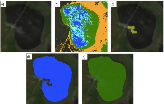
transformation function on the Sentinel 2 imagery between the approximately equivalent Landsat and Sentinel 2 bands (Zhang et al., 2018; Ahmad et al., 2019). The DSWE algorithm then is applied and classifies each pixel into one of five categories: high probability of water, moderate probability of water, low probability of water, not water, or wetland (Figure 4b). Pixels with a high or moderate level of confidence or classified as wetland are selected out to create the water mask over each lake (Figure 4d). We include wetland pixels due to the large amounts of
partially obscured by clouds, we employ a cloud filling algorithm. It fills in the cloud-created holes in the lake mask (Figure 4c) within the lake polygon boundary using the Pekel Surface Water Occurrence (SWO) Value (Pekel et al., 2016). The SWO value represents the frequency, between 1984 and 2015, that surface water was observed by Landsat. Wherever there is an occurrence value of 50% or more within the lake polygon boundary underneath the masked clouded area, the pixel is designated in as water (Figure 4e). Using a GEE function, we then calculate lake surface area for each lake image in the time series (Figure 3b).
Some outliers in the lake surface water timeseries do occur. Outliers, which are removed, are defined as being >25% from the median surface area value. In lakes with very high
variations in surface area this threshold might require adjustment, but the surface areas of lakes studied here are sufficiently stable to not require adjustment. After removing the outliers, the number of useable satellite images drops to 13,713. These images are matched to the lake level data to calculate variations in lake volume (See section 4.3). In general, the number of images used per lake varies due to differences in cloudiness and outlier removals (Ogilvie et al., 2018). 4.2.3 Validation
three lakes for the validation: Bay Tree Lake and Great Lake in eastern North Carolina and Lake Wenatchee in Washington. These lakes are chosen because they represent different test cases. Bay Tree Lake poses little difficulty when calculating lake surface area. Great Lake, however, contains extensive flooded vegetation, leading to omission and under detection of pixels when determining water pixels and calculating lake surface area. Lake Wenatchee also poses some difficulties when calculating lake surface area because it is located in the mountains and experiences topographic shadow and adjacent snow cover. We selected five dates from each lake’s surface area record that also had a corresponding lake level measurement and found the corresponding Planet image on that date. In two cases, images were matched plus or minus a day due to a gap in the Planet record or clouds. Some dates had two useable images due to
overlapping satellite orbits. In these cases, both were used and tested. This means that we include more than five comparisons between Planet Imagery and Landsat/S2 data per lake (Table A2). For the analysis, we first manually drew the lake boundary on each image, creating a lake polygon (Figure 5). Next, we calculated the surface area over that polygon using the Planet interface tool. Everything inside of the polygon is considered water, so the lake surface area is equivalent to the polygon area.
4.3 Measuring Lake Water Storage
Our overall strategy to calculate change in lake water storage was to develop a rating curve between lake stage and lake volume variations. We calculate the initial lake water volume using the lake level measurements collected by the citizen scientists and the surface area
variations from all lake stage measurements, rather than just when stage and area measurements are temporally coincident.
4.3.1 Calculation of Lake Water Storage
To calculate change in lake storage, or volume, over time, the lake water level
measurements for each of the lakes is combined with lake surface area measurements. If a lake level and a surface area measurement fall on the same day, they are automatically paired. If there are two lake level measurements on the same day a surface area measurement is calculated, we use the average of those two measurements. If there is no lake level taken on a day a surface area measurement is taken, then the nearest lake level measurement ± 1 day is used as a pairing. If there is a lake level measurement from the day before a well as one for the day after the image was collected, we average the lake level measurements. If there is no matching lake surface area measurement for a lake level measurement, or vice versa, that data is not used in calculating volume variations.
Lake volume change is then calculated for each date with a lake level and area pairing based on a linear equation that assumes lake volume change can be approximated by trapezoidal volume (eqn. 1),
𝑉 = ℎ
2∙ (𝐵1+ 𝐵2) (1) where V is volume, h is height, 𝐵1 is one base measurement of the trapezoid and 𝐵2is the other base measurement of the trapezoid. This basic equation can then be applied to capture the change in water volume for lakes (eqn. 2) (adapted from Quellec and Crétaux, 2018):
∆𝑉 (𝑡𝑖 𝑡𝑖0) =
[𝐵(𝑡𝑖)+𝐵(𝑡𝑖0)]
2 ∙ [ℎ(𝑡𝑖) − ℎ(𝑡𝑖0)], (2) where ∆𝑉 (𝑡𝑖
water surface area at the time of first image in the time series. The variable h(𝑡𝑖) is the height at time of image and h(𝑡𝑖0) is height of lake in the first image in the time series. Applying this equation to each level and area pair leaves us with a timeseries of variations in lake water volume for each lake (Figure 3c). Absolute volume cannot be calculated because lake bathymetry is unknown.
4.3.2 Rating Curve
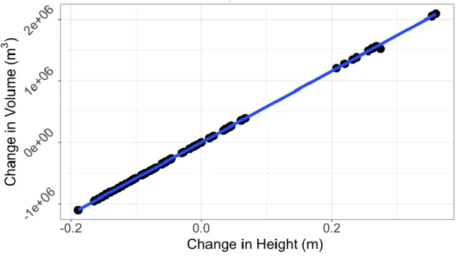
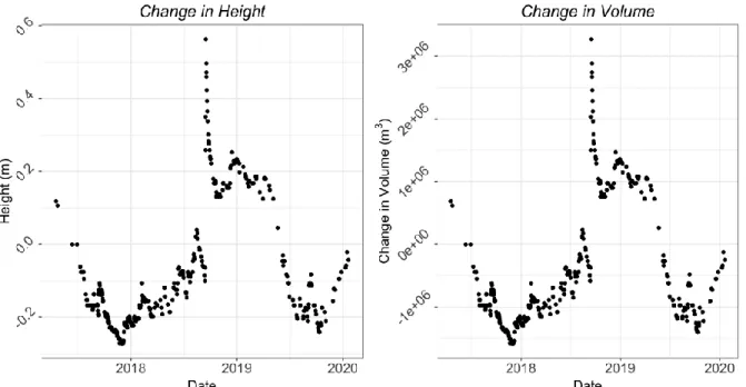
In order to maximize data usage for each lake, we used a rating curve approach to estimate variations in lake volume. This approach has been used by others (Medina et al., 2010; Liebe et al., 2013; Ogilvie et al., 2018). Ogilvie et al. (2018) noted that for most small lakes change in lake water volume primarily functions as a response to changes in lake water level; we made the same observation. To develop a stage-volume change rating curve for each lake, we regressed the calculated variations in lake water volume against the corresponding lake level measurements. A linear equation was determined for this relationship (Figure 6). The equation was then applied to all lake level measurements in the lake’s record to calculate a volume
variation timeseries (Figure 7). We used all lake pairs except those where a linear equation could not be calculated, meaning lakes with only one measurement.
4.3.3 Validation
science data (Figure 8). We then calculated Pearson’s Correlation Coefficient (r) between the pressure transducer data and the citizen science data timeseries.
4.4 Correlations between Change in Lake Water Storage 4.4.1 Calculating Correlations
Once variations in lake water storage are calculated for all lakes in all regions, we calculate the Spearman’s correlation coefficient () (Spearman, 1904) of those changes between all pairs of lakes in each region. We chose to use Spearman’s because it is less sensitive than a Pearson’s correlation to the assumption that relationships between paired lake water levels are linear. We did calculate Pearson’s correlation initially and noted no or only minor differences with Spearman’s . Observations for each lake are matched by date, or ± 1 day if no date match. If there are fewer than 10 paired measurements, a correlation coefficient was not calculated, and the lake to lake pair was not used. We used a threshold of n=10 to avoid a case where a very small number of observations led to a spurious correlation. However, we note that including all lakes does not substantially change our results. This analysis is repeated for all lake pairs in a region and completed separately for each of the four regions.
4.4.2 Validation
4.5 Spatial Analysis
To assess whether correlations in paired lake water storage are controlled by distance, we regressed the correlation coefficients described in section 4.4.1 against the distance between the pair of lakes associated with each correlation. We assess whether distance is a major control on correlation using the Spearman’s between paired lake distance and paired lake correlation coefficient.
5. Results
5.1 Validation Results 5.1.1 Citizen Science Data
Comparison of lake stage measurements made by citizen scientists against pressure transducers suggest that measurements by citizen scientists are highly accurate (Figure 9). Across 2,702 corresponding lake level measurements, we observe an r2 value of >0.99, a mean absolute error (MAE) of 1.6 cm, and a root mean squared error (RMSE) of 2.7 cm. The
measurement error of the pressure transducers is 0.8 cm. There are several outliers in the citizen science data, and we attribute most of these to data entry error by citizen scientists.
5.1.2 Lake Surface Area
more complicated case with inundated vegetation, the percent difference between the Landsat or Sentinel 2 imagery and the Planet imagery are virtually the same. This could be a result of including pixels classified as wetlands in our initial water mask. Lake Wenatchee is also a difficult case but for a different reason. Lake Wenatchee has topographic shadow that covers the lake at times due to the lake’s location in the Cascade Mountains. The values of topographically shadowed pixels in the imagery are similar to those of the water, leading to a modest
overestimation of surface water in our automatic Landsat and Sentinel 2 classifications compared to Planet imagery.
5.1.3 Lake Volume Correlations
Correlation coefficients between pairs of lakes are similar, though not identical, when computed using citizen science data and automated water level loggers (Figure 11). The Pearson’s correlation coefficient of 0.76 between paired lake correlation coefficients from the two different data sources, and the relative similarity of the best fit and one-to-one lines suggests that, in general, correlation coefficients from temporally sparse citizen science data are likely reliable. The average difference in correlation coefficients between the two methods is 0.23. There is no relationship between sample size and difference between citizen science-based and pressure transducer-based correlation coefficients in any of the lake regions (Figure A1). 5.2 Variations in Lake Water Storage
5.2.1 Correlation between the Change in Lake Water Volume
substantial spread in the degree of correlation, with some pairs of lakes highly correlated and others uncorrelated. For example, storage variations in Bay Tree Lake and Salters Lake are highly correlated, Bay Tree Lake and Lake Mattamuskeet East are moderately correlated, and Bay Tree Lake and Lake Waccamaw are only slightly correlated (Figure 13).
5.2.2 Correlations and Relationship with Distance
There is a weak relationship between distance and paired lake correlation in two regions (North Carolina and Wisconsin) and no significant relationship in the other two regions
(Washington and Illinois) (Figures 14b – 14e). When lakes in all regions are combined, there is a weak but statistically significant relationship between distance and paired lake correlation (Figure 14a).
To test whether the correlations are influenced by the number of paired measurements, we plot the number of measurements against the correlation coefficients between each lake. There is no relationship between the number of measurements and the strength of correlation, in all of the regions combined or in any region individually (Figure 15). We also test whether the variability in paired lake correlation increases with paired lake distance. We plot the distance between paired lakes and the residual from the best fit lines in Figure 16. The results show there is not a strong relationship and that spread is uniform as distance increases. There is a slight, but significant (p = <0.01), negative relationship in North Carolina and positive relationship in Illinois (Figure 16).
6. Discussion
transducer lake level data, with the primary difference being that the pressure transducer data captures a more detailed timeseries. The lake surface areas automatically calculated from
Landsat and Sentinel 2 imagery are quite similar to the areas manually calculated from the Planet imagery. For simple cases like Bay Tree Lake (Figure 5a), as well as lakes affected by inundated vegetation, like Great Lake (Figure 5b), lake surface areas compare very well to manually digitized maps made from same-day, high-resolution Planet imagery. For cases where topographic shadows are important, like Lake Wenatchee (Figure 5c), lake surface area is overestimated in the automated classifications, likely due to topographic shadow pixels misclassified as water. In general, the Planet imagery has a finer spatial resolution than that of the Landsat and Sentinel 2 imagery, meaning that Planet imagery can capture more
heterogeneity. This decreases much shoreline pixel error that might be occurring with the Landsat and Sentinel 2 imagery, and Planet imagery can detect subtle changes in inundation extent not apparent in Landsat or Sentinel 2 imagery (Cooley et al., 2019). It is important to note that there could still be error in the Planet imagery surface area delineations, due to user error in the manual delineation. Ultimately, there is no ‘absolute truth’ when measuring surface area through satellite imagery (Ogilvie et al., 2018). Overall, our results suggest that citizen science data and optical satellite imagery accurately capture changes in lake water storage.
been driven by net atmospheric flux as well as stage-dependent outflow. Euliss & Mushet (1996) found that, during one spring and summer season, water level fluctuations are greater in wetlands with more agricultural activity, rather than grasslands, and that water level fluctuations in
semipermanent wetlands are more stable due to the inputs of groundwater, whereas seasonal and temporary wetlands solely depend on runoff. Correlations between surface area in small lakes and their sub-seasonal dynamics has been studied by Cooley et al., (2019) across Alaska and the Canadian Shield. They note that, as a whole, lake surface area is declining across all study regions, with some distinct localized exceptions, which primarily reflects negative net summer atmospheric flux in North America in 2017. They also note that the change in surface area seen is primarily driven by lake level fluctuation, not shoreline vegetation growth. The study
presented here begins to provide a baseline in the level of correlation we may expect to see in the changes of lake water storage between lakes in a region, at least on timescales of 1-2 years. Perhaps surprisingly, the average correlation between pairs of lakes within our four study regions is only moderately positive (=0.49) and highly variable. This result suggests that measurements made in one lake provide some regional information, but that, at least in the regions we
years, not several decades, and those trends cannot be captured. This study would need to be continued for many more years in order to capture those patterns.
Perhaps just as surprising, we observed only limited correlation between paired lake Spearman’s and paired lake distance. The idea that as the distance between lakes increases, the correlation of change in lake water storage between those two lakes decreases, is an intuitive one. However, the results from this study provide only limited evidence for this relationship. When aggregated together across all regions, our data shows a significant but weak correlation (=-0.21). Two regions, Illinois and Washington, show slightly stronger negative relationships between correlation and distance (=-0.44 and -0.34, respectively), while North Carolina and Wisconsin show no significant relationship between correlation and distance. We also tested for any relationship between the variation in paired lake correlation (as measured by the absolute value of residuals) and distance but found no statistically significant relationship in any region. All of this suggests that, when thinking about the spatial synchrony between the change in lake water storage of the lakes, there are other factors in play that are more important than distance.
period—for example, the large spike in water levels in Bay Tree Lake (Figure 3) is the result of Hurricane Florence, which impacted some North Carolina lakes much more than others. Our results suggest that, at least in the places and over the time periods studied here, both regional and lake-specific factors matter a great deal in driving variations in lake water storage.
While the results of this study represent a first analysis of lake-to-lake water storage correlation across many lakes, there is still a great deal that we do not understand about the drivers of lake water levels. Some relevant questions will be addressed after the launch of the upcoming SWOT satellite mission in 2022 (Biancamaria et al. 2016). Because SWOT will measure lakes as small as 250 m by 250 m, it will provide time series of variations in water storage for millions of lakes globally. Continuing measurements from LOCSS and other sources based on citizen science and satellite imaging will provide key ground truthing data for SWOT, especially in areas where there is limited on-the-ground measurement available.
Overall, this study addresses a gap in understanding about lake water storage. Here we suggest that change in lake water volume in small lakes can accurately be monitored by
TABLES Table 1. Table of study site properties.
North Carolina Washington State Illinois Wisconsin
Number of Lakes 12 22 17 32
Minimum Lake Size 0.89 km2 0.064 km2 0.059 km2 0.051 km2
Maximum Lake Size 103 km2 89 km2 0.979 km2 39.612 km2
Satellite Images Available
(1/1/2015 – 2/1/2020)
1,566 4,701 2,298 5,148
Lake Level Measurements
(Start of citizen science record – 2/1/2020)
2,047 1,390 876 960
Starting Dates April 18th, 2017
September 10th, 2018
May 13th, 2019
APPENDIX: SUPPLEMENTAL INFORMATION Table A1. Individual Lake Properties
Lake Name Region
Approx. Size (km2)
Date of First Lake Level Measurement
Date of Last Lake Level Measurement Used Number of Lake Level Measurements
(Start of citizen science record –
2/1/2020) Number of Satellite Images (1/1/2015 – 2/1/2020) Bay Tree
Lake NC 5.8 4/18/17 1/20/20 389 114
Catfish Lake NC 3.8 9/19/17 5/22/19 42 203
Great Lake NC 11.3 9/19/17 1/10/20 47 147
Horsepen
Lake NC 1.2 9/21/17 1/20/20 209 113
Jones Lake NC 0.9 4/18/17 2/1/20 154 112
Lake Mattamuskeet
West
NC 57.6 6/1/17 1/27/20 140 120
Phelps Lake NC 64.5 6/1/17 1/25/20 295 109
Salters Lake NC 1.3 4/18/17 2/1/20 144 189
Singletary
Lake NC 2.3 4/18/17 1/30/20 106 113
Lake Mattamuskeet
East
NC 105.7 6/1/17 1/27/20 139 120
Lake
Waccamaw NC 35.8 4/18/17 1/19/20 260 112
White Lake NC 4.3 4/18/17 12/25/19 122 114
Beaver Lake WA 0.3 9/10/18 1/25/20 59 71
Walupt Lake WA 1.5 6/12/19 10/30/19 21 176
Bosworth
Lake WA 0.4 9/12/18 1/28/20 26 249
Lake Cassidy WA 0.5 9/12/18 10/26/19 38 249
Coldwater
Lake WA 3.0 6/11/19 2/1/20 62 88
Deep Lake WA 0.2 6/10/19 11/28/19 44 82
Dog Lake WA 0.2 6/13/19 10/30/19 10 254
Echo Lake WA 0.06 9/12/18 10/30/19 69 167
Fish Lake WA 2.0 6/12/19 1/24/20 24 187
Lake Howard WA 0.1 6/11/19 12/10/19 10 305
Lake
Lawrence WA 1.3 9/12/18 2/1/2020 66 273
Leech Lake WA 0.2 6/13/19 12/05/19 35 263
Phantom
Lake WA 0.3 9/10/18 1/31/20 167 164
Crabapple
Lake WA 0.1 6/11/19 08/26/19 9 267
Lake
Roesiger WA 1.4 9/10/18 1/28/20 30 237
Lake
Sammamish WA 19.6 9/11/18 1/30/20 193 152
Steel Lake WA 0.2 6/10/19 1/31/20 127 152
Flowing Lake WA 0.5 9/10/18 1/28/20 49 253
North Lake WA 0.2 6/10/19 2/1/20 53 142
Lake
Washington WA 89.0 10/11/18 2/1/20 139 178
Lake
Wenatchee WA 9.7 9/10/18 1/25/20 69 185
Lake Martha WA 0.2 9/13/18 1/26/20 80 295
Diamond
Lake IL 0.6 5/16/19 11/23/19 28 86
Lake
Defiance IL 0.3 5/15/19 12/26/19 62 69
Gages Lake IL 0.6 5/13/19 11/23/19 29 165
Hastings Lake IL 0.3 5/14/19 1/11/20 121 168
Herrick Lake IL 0.05 5/23/19 1/31/20 109 88
Harrier Lake IL 0.08 5/29/19 11/21/19 29 84
Lake
Killarney IL 0.2 5/15/19 12/11/19 26 89
Highland
Lake IL 0.4 5/14/19 9/21/19 26 167
East Loon
Lake IL 0.8 5/14/19 1/15/20 49 158
West Loon
Lake IL 0.7 5/14/15 1/15/20 49 172
Lily Lake IL 0.4 5/15/19 12/17/19 29 87
McCullom
Lake IL 1.0 5/15/19 11/5/19 18 128
Maple Lake IL 0.2 5/16/19 1/11/20 29 167
Deep Quarry
Lake IL 0.1 5/29/19 11/5/19 43 82
Round Lake IL 1.0 5/14/19 12/26/19 82 168
Silver Lake IL 0.2 5/16/19 1/1/20 37 87
Timber Lake IL 0.3 5/14/19 12/26/19 50 170
Archibald
Lake WI 1.6 4/26/16 5/7/19 92 157
Axhandle
Lake WI 0.3 7/13/15 10/5/17 29 161
Bass Lake WI 0.3 08/13/15 10/20/16 40 85
Bear Lake WI 0.1 6/22/17 11/03/17 12 123
Big Twin
Lake WI 0.3 7/15/16 5/4/19 61 155
Clear Lake WI 0.3 6/21/17 11/30/17 24 90
Crystal Lake WI 0.1 07/14/17 9/21/17 10 64
Deep Lake WI 0.1 06/17/17 07/06/17 3 220
Des Moines
Lake WI 0.9 4/18/17 11/02/17 28 175
Duck Lake WI 0.5 7/5/16 9/23/19 82 225
Grindle Lake WI 0.2 11/9/15 8/10/19 91 169
Horseshoe
Lake WI 1.6 8/18/15 6/6/19 72 244
Kentuck Lake WI 4.0 7/5/19 7/5/19 1 151
Kilby Lake WI 0.2 5/20/17 10/1/17 41 146
Lake Five WI 0.4 5/23/17 10/3/17 19 166
Long Lake WI 1.1 8/18/15 8/19/19 58 249
Loon Lake WI 0.1 8/14/2015 10/20/16 22 148
Mann Lake WI 1.0 5/12/18 5/12/18 1 85
Moose Lake WI 0.5 8/6/16 9/29/18 5 121
Parker Lake WI 0.2 6/10/17 9/16/17 14 225
Paya Lake WI 0.4 11/9/15 9/20/19 65 157
Phantom
Lake WI 0.2 8/19/15 11/6/15 16 86
Poplar Lake WI 0.5 6/30/18 9/11/19 10 250
Sand Lake WI 3.6 4/18/17 7/26/17 15 171
South Neva
Lake WI 0.1 8/30/15 11/21/16 24 240
Spur Lake WI 0.5 7/29/19 9/24/19 13 126
Stratton Lake WI 0.3 7/11/17 9/21/17 10 82
Summit Lake WI 1.1 4/5/19 9/6/19 18 224
Twin Lakes WI 0.05 6/11/17 10/01/17 16 214
Underwood
Lake WI 0.2 8/24/15 5/7/19 9 161
Wheeler Lake WI 1.1 8/26/15 5/7/19 46 157
Table A2. Differences in automated Landsat and Sentinel 2 surface area calculations and those manually delineated from Planet Imagery on the corresponding days.
Lake Date of Landsat or Sentinel 2 image Automated Lake Surface Area from Landsat and
Sentinel 2 Imagery (km2) Date of Planet Imagery Manual Lake Surface Area from Planet Imagery (km2) Difference
BTN2 2020-01-20 5.806 2020-01-20 5.861 -0.055
BTN2 2020-01-20 5.806 2020-01-20 5.881 -0.075
BTN2 2019-06-24 5.789 2019-06-24 5.871 -0.082
BTN2 2019-06-24 5.789 2019-06-24 5.882 -0.093
BTN2 2018-08-25 5.806 2018-08-25 5.874 -0.068
BTN2 2018-08-25 5.806 2018-08-25 5.857 -0.051
BTN2 2018-01-14 5.883 2018-01-14 5.863 0.02
BTN2 2017-07-21 5.806 2017-07-21 5.881 -0.075
BTN2 2017-07-21 5.806 2017-07-21 5.881 -0.075
GRN2 2019-08-21 11.372 2019-08-21 11.477 -0.105
GRN2 2019-01-09 11.523 2019-01-09 11.544 -0.021
GRN2 2018-07-08 11.391 2018-07-09 11.514 -0.123
GRN2 2018-07-08 11.391 2018-07-09 11.543 -0.152
GRN2 2017-12-21 11.478 2017-12-21 11.559 -0.081
GRN2 2017-10-02 11.422 2017-10-02 11.594 -0.172
WEW2 2019-08-20 9.751 2019-08-20 9.518 0.233
WEW2 2019-06-02 10.009 2019-06-02 9.656 0.353
WEW2 2019-06-02 10.009 2019-06-02 9.676 0.333
WEW2 2019-04-30 10.28 2019-04-30 9.63 0.65
WEW2 2019-04-30 10.28 2019-04-30 9.819 0.461
WEW2 2019-01-26 9.985 2019-01-26 9.67 0.315
WEW2 2019-03-30 10.003 2019-03-30 9.68 0.323
REFERENCES
Abarca-del- Río, R., Crétaux, J-F., Berge-Nguyen, M., & Maisongrande, P. (2012). Does the Titicaca Lake still control the Poopo lake water levels? An investigation using satellite altimetry, and MODIS data (2000–2009). Remote Sens. Lett., 3(8), 707–714.
https://doi.org/10.1080/01431161.2012.667884
Adrian, R., O'Reilly, C. M., Zagarese, H., Baines, S. B., Hessen, D. O., Keller, W., Livingstone, D. M., Sommaruga, R., Straile, D., Van Donk, E., Weyhenmeyer, G. A., & Winder, M. (2009). Lakes as sentinels of climate change. Limnology and oceanography, 54(6), 2283– 2297. https://doi.org/10.4319/lo.2009.54.6_part_2.2283
Ahmad, S.K., Hossain, F., Eldardiry, H., & Pavelsky, T.M. (2019). A Fusion Approach for Water Area Classification using Visible, Near Infrared and Synthetic Aperture Radar for South Asian Conditions. IEEE Transactions on Geoscience and Remote Sensing, 58(4), 2471 – 2480. https://doi.org/10.1109/TGRS.2019.2950705
Alsdorf, D.E., Birkett, C.M., Dunne, T., Melack, J., & Hess, L. (2001). Water level changes in a large Amazon lake measured with spaceborne radar interferometry and altimetry.
Geophys. Res. Lett., 28(14), 2671–2674. https://doi.org/10.1029/2001GL012962
Annor, F. O., van de Giesen, N., Liebe, J., van de Zaag, P., Tilmant A., & Odai, S. (2009). Delineation of small reservoirs using radar imagery in a semi-arid environment: A case study in the upper east region of Ghana. Phys. Chem. Earth Pt. A/B/C, 34, 309-315. https://doi.org/10.1016/j.pce.2008.08.005
Arsen, A., Crétaux, J-F., Berge-Nguyen, M., & Abarca-del-Rio, R. (2014). Remote sensing derived bathymetry of Lake Poopo. Remote Sens., 6(1), 407–420.
https://doi.org/10.3390/rs6010407
Arsen, A., Crétaux, J-F. & Abarca-del-Rio, R. (2015). Use of SARAL/AltiKa over Mountainous Lakes, Intercomparison with Envisat Mission. Marine Geodesy, 38, 00-00.
https://doi.org/10.1080/01490419.2014.1002590.
Avisse, N., Tilmant, A., Muller, M. F., & Zang, H. (2017). Monitoring small reservoirs’ storage with satellite remote sensing in inaccessible areas. Hydrol. Earth Syst. Sci., 21, 6445-6459. https://doi.org/10.5194/hess-21-6445-2017
Baup, F., Frappart, F., & Maubant, J. (2014). Combining high-resolution satellite images and altimetry to estimate the volume of small lakes. Hydrol. Earth Syst. Sci., 18, 2007-2020. https://doi.org/10.5194/hess-18-2007-2014
Biancamaria, S., Lettenmaier, D.P., & Pavelsky, T.M. (2016). The SWOT Mission and Its Capabilities for Land Hydrology. Surv.Geophys., 37(2), 307-337.
Bretz, J. H. (1910). Glacial lakes of Puget Sound. Journal of Geology. 18, 448-458. Bretz, J. H. (1913). Glaciation of the Puget Sound region. Washington Geological Survey
Bulletin, 8, 244.
Bryant, R.G. (1999). Application of AVHRR to monitoring a climatically sensitive playa. case study: Chott El Djerid, Southern Tunisia. Earth Surface Processes and Landforms, 24(4), 283-302.
https://doi.org/10.1002/(SICI)1096-9837(199904)24:4<283::AID-ESP950>3.0.CO;2-9
Booth, D. B. (1990). Surficial geologic map of the Skykomish and Snoqualmie rivers area, Snohomish and King counties, Washington. The Survey.
Buytaert, W., Zulkafli, Z., Grainger, S., Acosta, L., Alemie, T.C., Bastiaensen, J., Bievre, B.D., Bhusal, J., Clark, J., Dewulf, A., Foggin, M., Hannah, D.M., Hergarten, C., Isaeva, A., Karpouzoglou, T., Pandeya, B., Paudel, D., Sharma, K., Steenhuis, T., Tilahun, S., Hecken, G.V., & Zhumanova, M. (2014). Citizen Science in hydrology and water resources: opportunities for knowledge generation, ecosystem service management, and sustainable development. Front. Earth Sci., http://doi.org/10.3389/feart.2014.00026 Calmant, S., Seyler, F., & Crétaux, J-F. (2008). Monitoring continental surface waters by
satellite altimetry. Surv. Geophys., 29(4–5), 247–269. http://doi.org/10.1007/s10712-008-9051-1
Canfield, D.E., Brown, C.D., Bachmann, R.W., & Hoyer, M.V. (2002). Volunteer lake monitoring: testing the reliability of data collected by the Florida lakewatch program. Lake Reserv. Manag., 18, 1–9. https://doi.org/10.1080/07438140209353924
Coe, M., & Foley, J. (2001). Human and natural impacts on the water resources of the Lake Chad Basin. Journal of Geophysical Research., 106, 3349-3356.
https://doi.org/10.1029/2000JD900587
Cooley, S.W., Smith, L.C., Stephan, L., & Mascaro, J. (2017). Tracking Dynamic Northern Surface Water Change with High-Frequency Planet CubeSat Imagery. Remote Sens. 9(12), 1306. https://doi.org/10.3390/rs9121306
Cooley S.W., Smith, L.C., Ryan, J.C., Pitcher, L.H., & Pavelsky, T.M. (2019). Arctic-Boreal Lake Dynamics Revealed Using CubeSat Imagery. Geophys. Res. Lett., 46(4).
https://doi.org/10/1029/2018GL081584
Cohen, J. P. (2008). “Citizen science: Can volunteers do real research?” BioScience, 58(3), 192. https://doi.org/10.1641/B580303
Crétaux, J.-F., Abarca-del-Río, R., Bergé-Nguyen, M., Arsen, A., Drolon, V., Clos, G., &
Davis, C. A. (1971). Discovered: eleven global forces. Unpublished manuscript. Marietta, Ohio. Dickinson, J. L., Shirk, J., Bonter, D., Bonney, R., Crain, R. L., Martin, J., Phillips, T., &
Purcell, K., (2012). The current state of citizen science as a tool for ecological research and public engagement. Front. Ecol. Environ., 10, 291–297.
https://doi.org/10.1890/110236
Downing, J.A., Prairie, Y.T., Cole, J.J., Duarte, C.M., Tranvik, L.J., Striegl, R.G., McDowell, W.H., Kortelainen, P., Caraco, N.F., Melack, J.M., & Middelburg, J. (2006). The global abundance and size distribution of lakes, ponds, and impoundments. Limnol. Oceanogr., 51, 2388–2397. https://doi.org/10.4319/lo.2006.51.5.2388
Downing, J.A. (2009). Emerging global role of small lakes and ponds: little things mean a lot. Limnetica, 29 (1), 9-24. https://doi.org/10.23818/limn.29.02
Duan, Z., & Bastiaanssen, W.G.M. (2013). Estimating water volume variations in lakes and reservoirs from four operational satellite altimetry databases and satellite imagery data. Remote Sens. Environ., 134, 403–416. http://doi.org/10.1016/j.rse.2013.03.010
Euliss, N. H., & Mushet, D. M. (1996). Water-level fluctuation in wetlands as a function of landscape condition in the prairie pothole region. Wetlands, 16(4), 587-593.
Fekete, B. M., Robarts, R. D., Kumagai, M., Nachtnebel, H.-P., Odada, E., & Zhulidov, A. V. (2015). Time for in situ renaissance. Science, 14, 685-686.
http://doi.org/10.1126/science.aac7358
Fienen, M.N., & Lowery, C.S., (2012). Social.Water—A crowdsourcing tool for environmental data acquisition. Computers and Geosciences, 49, 164 - 169.
https://dx.doi.org/10.1016/j.cageo.2012.06.015
Gao, H., Birkett, C.M., & Lettenmeir, D.P. (2012). Global monitoring of large reservoir storage from satellite remote sensing. Water Resour. Res., 48, W09504.
http://doi.org/10.1029/2012WR012063
Gardelle, J., Hiernaux, P., Kergoat, L., & Grippa, M. (2010). Less rain, more water in ponds: a remote sensing study of dynamics of surface waters from 1950 to present in pastoral Sahel (Gourma region, Mali), Hydrol. Earth Syst. Sci., 14, 309-324. https://doi.org/10. 5194/hess/-14-309-2010
Gorelick, N., Hancher, M., Dixon, M., Ilyushchenko, S., Thau, D., & Moore, R. (2017). Google Earth Engine: Planetary-scale geospatial analysis for everyone. Remote Sens.
Grippa, M., Rouzies, C., Biancamaria, S., Blumstein, D., Crétaux, J.-F., Gal, L., Robert, E., Gosset, M., Kergoat, L. (2019). Potential of SWOT for Monitoring Water Volumes in Sahelian Ponds and Lakes. IEEE Journal of Selected Topics in Applied Earth
Observations and Remote Sensing, 12(7), 2541-2549. https://doi.org/10.1109/JSTARS.2019.2901434
Gupta, R. P., & Banerji, S. (1985). Monitoring of reservoir volume using LANDSAT data. Journal of Hydrology, 77(1-4), 159-170. https://doi.org/10.1016/0022-1694(85)90204-5
Hannah, D.M., Demuth, S., van Lanen, H.A.J., Looser, U., Prudhomme, C., Rees, R., Stahl, K., & Tallaksen, L.M. (2011). Large-scale river flow archives: importance, current status and future needs. Hydrol. Process., 25, 1191-1200. https://doi.org/10.1002/hyp.7794 Hanson, P. C., Carpenter, S. R., Cardille, J.A., Coe, M.T., & Winslow, L. A., (2007). Small lakes
dominate a random sample of regional lake characteristics. Freshw. Biol., 52, 814– 822. https://doi.org/10.1111/j.1365-2427.2007.01730.x
Hunter, J., Alabri, A., & van Ingen, C. (2012). Assessing the quality and trustworthiness of citizen science data. Concurrency and Computation: Practice and Experience, 25(4). https://doi.org/10.1002/cpe.2923
Hughes, D.A. (2006). Comparison of satellite rainfall data with observations from gauging station networks. Journal of Hydrology, 327, 399–410.
https://doi.org/10.1016/j.jhydrol.2005.11.041
IAHS Ad Hoc Group on Global Water Data Sets. (2001). Global water data: A newly endangered species. Eos Trans AGU, 8, 54-58. https://doi:10.1029/01EO00031
IPCC. (2014). Intergovernmental Panel on Climate Change Fifth Assessment Report. Retrieved from http://www.ipcc.ch/.
Irwin, A. (2018). Citizen Science Comes of Age. Nature. 562, 480 – 482. https://10.1038/d41586-018-07106-5
Izhitskiy, A. S., Zavialov, P. O., Sapozhnikov, P. V., Kirillin, G. B., Grossart, H. P., Kalinina, O. Y., Zalota, A.K., Goncharenko, I.V., & Kurbaniyazov, A. K. (2016). Present state of the Aral Sea: diverging physical and biological characteristics of the residual basins.
Scientific Reports, 6(1), 1-9. https://doi.org/10.1038/srep23906
Jeppesen, E., Brucet, S., Naselli-Flores, L., Papastergiadou, E., Stefanidis, K., Noges, T.,
Attayde, J.L., Zohary, T., Coppens, J., Bucak, T., Menezes, R.F., Freitas, F.R.S., Kernan, M., Sondergaard, M., & Beklioglu, Meryem. (2015). Ecological impacts of global
warming and water abstraction on lakes and reservoirs due to changes in water level and related changes in salinity. Hydrobiologia, 750(1), 201-227.