Infrastructure-less Occupancy Detection and Semantic
Localization in Smart Environments
Md Abdullah Al Hafiz Khan, H M Sajjad Hossain, Nirmalya Roy
Department of Information SystemsUniversity of Maryland Baltimore County
[email protected], [email protected], [email protected]
ABSTRACT
Accurate estimation of localized occupancy related informa-tion in real time enables a broad range of intelligent smart environment applications. A large number of studies using heterogeneous sensor arrays reflect the myriad requirements of various emerging pervasive, ubiquitous and participatory sensing applications. In this paper, we introduce a zero-configuration and infrastructure-less smartphone based lo-cation specific occupancy estimation model. We opportunis-tically exploit smartphone’s acoustic sensors in a conversing environment and motion sensors in absence of any conver-sational data. We demonstrate a novel speaker estimation algorithm based on unsupervised clustering of overlapped and non-overlapped conversational data and a change point detection algorithm for locomotive motion of the users to infer the occupancy. We augment our occupancy detection model with a fingerprinting based methodology using smart-phone’s magnetometer sensor to accurately assimilate
loca-tion informaloca-tion of any gathering. We postulate a novel
crowdsourcing-based approach to annotate the semantic lo-cation of the occupancy. We evaluate our algorithms in
dif-ferent contexts; conversational, silence and mixed in
pres-ence of 10 domestic users. Our experimental results on
real-life data traces in natural settings show that using this hybrid approach, we can achieve approximately 0.76 error count distance for occupancy detection accuracy on aver-age.
Categories and Subject Descriptors
H.4 [Mobile Systems and Applications]: Miscellaneous
Keywords
Crowdsourcing, Opportunistic sensing, Occupancy count-ing, Semantic Localization
1.
INTRODUCTION
Localized commercial (University, Office, Mall, Cineplex,
Restaurant etc.) and residential (apartment, home etc.)
.
building occupancy detection and estimation at room/zone level granularity in real time can provide meaningful insights to many smart environment applications, such as green build-ing, social gatherbuild-ing, event management etc. Smartphone-based participatory and citizen sensing applications have adhered to the promise of building such applications by uti-lizing various context sensing sensors on board. Different sensors can be exploited individually or in tandem to build a variety of such novel applications to satisfy the myriad re-quirements of differing smart environment applications. For example, potential benefit from microphone sensor based ap-plication is the assessment of social interaction and active engagement among a group of people by leveraging their conversational contents [1], speaker identification and
char-acterization of social settings [2][3][4]. To enumerate the
number of people in a conversational episode, such as dur-ing a social gatherdur-ing, interactive lecture session or in a restaurant or shopping mall environment, various speaker counting paradigms have been explored [5][6][7]. Most of the recent studies which focus on conversational data fea-tures to extract high level occupancy information, assume that all of the users need to take turns at some point. While this specific scenario is feasible it is not ideal. To tackle this ideal situation, researchers have proposed using arrays of microphone sensors, video cameras or motion sensors for identifying microscopic occupancy information in real time [8][9] which are obtrusive in nature. We envision to move one step further by considering a more natural environ-ment where people may spontaneously participate or abstain from any conversational phenomenon. We posit to augment smartphone-based locomotive sensing model in absence of any conversational episode along with acoustic sensing-based audio inference model to precisely capture the characteris-tic of a natural environment and accurately estimate the
occupancy count. To further pinpoint the occupancy we
integrate the smartphone’s magnetometer sensor-based lo-cation sensing model. In pursuit of these goals we design a model which opportunistically exploits both the audio and motion data respectively from smartphone’s microphone and accelerometer sensor to infer the number of people present in a gathering and their semantic location information as sup-plemented by the magnetometer sensor on the smartphone. We also introduce a crowdsourcing model to reduce the ef-fort for obtaining semantic location information at scale.
In particular we propose a zero-hassle ambient and in-frastructure-less mobile sensing (aka smartphone) based ap-proach by exploiting only the smartphone’s sensors to pro-vide significantly greater visibility on real time occupancy
MOBIQUITOUS 2015, July 22-24, Coimbra, Portugal Copyright © 2015 ICST
and its semantic location. The key challenge in this case is to effectively estimate the number of people in a crowded and non-crowded environment either in presence of any con-versational data or not. Such hybrid sensing approach could potentially furnish more fine-grained occupancy profiling to better serve many participatory sensing applications while saving smartphones’ battery power by advocating a distributed sensing strategy. Main contributions of the paper are sum-marized below:
• We propose an acoustic sensing based linear time
adap-tive people counting algorithm based on real-life con-versational data which promotes a unified strategy of considering both overlapped and non-overlapped con-versational data in a natural environment. We propose to select opportunistically minimal number of micro-phone sensors which can substantially reduce the en-ergy consumption of smartphones. Our proposed peo-ple counting algorithm can dynamically select length of the audio segment compared to the other existing work [6].
• Although acoustic sensing based approach holds great
promises in inferring the number of occupants it fails in absence of any conversational data. Therefore we pro-pose to augment motion sensing based counting strat-egy with our acoustic sensing based people counting algorithm which works on extreme modality of either of the data sources, be it acoustic or locomotive.
• We design a magnetometer sensor based localization
technique at zone/room level granularity to infer the location of a conversing group. We propose a novel crowdsourcing model to map the magnetic signature of different locations and collect a large number of anno-tated location information to tag the occupancy with its semantic location information.
2.
RELATED WORK
We particularly review the most relevant literatures on occupancy inference problem in the context of conversa-tional sensing, localization, and speaker estimation which are smartphone based.
Smartphone Speaker Sensing: A large number of prior work have used smartphones’ microphone to
opportunisti-cally analyze audio for context characterization. For
ex-ample, SpeakerSense [4] performs speaker identification and SoundSense [10] classifies sounds from macro to micro con-texts. They have often in common employing the supervised speaker learning techniques. In contrast, our model’s occu-pancy counting process is entirely unsupervised. Our pro-posed model anonymously estimates the number of people from smartphones’ acoustic cum locomotive sensing model where we have employed unsupervised learning techniques to cluster different forms of acoustic signatures. For exam-ple, [11] have built a model from mean and covariance matri-ces of Linear Predictive Cepstral Coefficient (LPCC) of voice segments in conversations and used Mahalanobis distance to determine if two models belong to the same or different speakers. [12] has performed speaker clustering using dis-tance of the feature vectors extracted from different speak-ers and finally applied modified C-means algorithm with distance metric data. However, their experiments for oc-cupants estimation were on telephonic conversational data,
where multiple participants were present, and voices were frequently overlapped and intertwined with the noisy en-vironment. Our proposed model performs speaker count-ing without any predefined environmental setup and col-lects data from natural conversation. Our proposed speaker counting algorithm is close to [13], [6] where smartphone-based speaker counting has been proposed in a controlled scenario where all the participants spoke actively. [6] used a fixed length audio segment (3 sec) where each segment corresponds to an individual but we performed this audio segmentation dynamically to increase the accuracy of occu-pancy inference. [6] also classified a few segments as mined but our system never discards segments as undeter-mined which is achieved only through employing dynamic segmentation. Therefore, our proposed audio based occu-pancy inference model tackles a richer problem, where none of the speakers are discarded for handling the computational challenges. Crowd++ [6] proposed to combine pitch with MFCC to compute the number of people with an average error distance of 1.5 speakers. On the other hand our model improved the average error distance by a factor of two (0.76 Speakers).
Indoor Localization:UnLoc [14] proposed an unsuper-vised indoor localization approach exploiting environmental identifiable artifacts and specific signatures on single or mul-tiple sensing dimensions using smartphones’ different sensors readings (mainly from accelerometer, compass, gyroscope, and WiFi APs). [15] measured geomagnetic field in a way which is spatially varying but temporally stable, using an array of e-compasses to infer location. However they used a bunch of sensors or sensor arrays for location detection where as our model only used smartphones’ magnetometer sensor to infer semantic location information of a gather-ing at zone/room level granularity. [16] used magnetic fin-gerprints with dynamic time-warping algorithm to predict location information with a 92% accuracy. Our model used standard Random Forest algorithm and achieved 98% accu-racy to detect high level semantic location information of any gathering. IndoorAtlas location technology [17] utilized anomalies of ambient magnetic fields for indoor position-ing. This platform provides the functionality for participa-tory sensing where the crowd can contribute by war driving magnetic signatures of an unexplored location.
3.
OVERALL SYSTEM ARCHITECTURE
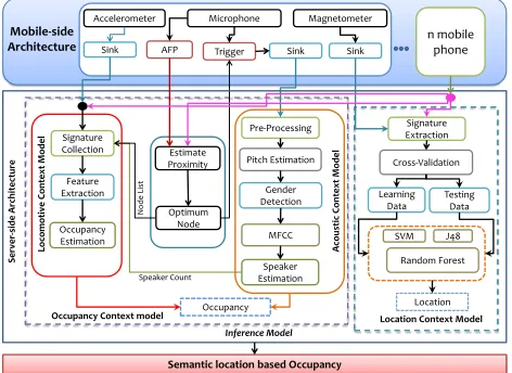
We envision developing a minimally invasive cost free ro-bust mobile system for counting the number of people present at any time in any environment and enlighten their seman-tic location information. Our model boosts these capabili-ties by employing smartphones’ magnetometer, microphone and accelerometer sensors. Our system as shown in Fig. 1, comprises of two subsystems, one deployed on smartphone and other in server. Using only acoustic sensing it is not al-ways possible to predict the correct number of the occupants present in a specific location as some people get involved in a conversation while others remain silent. For example, in a class room scenario while professor lectures some of the stu-dents participate but majority of the stustu-dents remain silent.
Sensed data are stored in a data sink (sink) for posterior
sensing for occupancy detection. For this joint collaborative sensing acoustic sensed data is being fed to the filter to col-lect Acoustic Fingerprint (AFP), consisting of content based audio. The AFPs being collected from all smartphones are
sent to “Estimate Proximity” module residing on the server
which helps distinguish the audio signals in vicinity and ap-proximate the inclusion of a group of smartphones to form
a single clique. Finally, “Optimum Node” module elects the
clique leader (most informative smartphone) to record the audio data and notifies the condition of deactivation to the other smartphones from capturing the duplicate audio sig-nal. It also helps in sorting the smartphone list based on their audio signal strength which is eventually utilized by lo-comotive “Signature Collection” module to opportunistically check-on and trigger the accelerometer sensor on the
smart-phones [18]. The server-side architecture consists of two
main logical sub-components:i)Occupancy Context Model,
and ii) Location Context Model. These models together
form the inference engine of our proposed semantic location sensitive occupancy detection system.
3.1
Occupancy Context Model
It has two sub-modules, Acoustic Context Model and Lo-comotive Context Model.
3.1.1
Acoustic Context Model (ACM)
Our acoustic context model comprises of the following three modules.
Pre-processing: This module is the most trivial phase for acoustic signal processing. This module helps to per-form the filtering and select the audio segment length dy-namically. It finally helps remove all the noises, silences and produce smooth conversational data which is later passed to the feature extraction module.
Feature Extraction: This is the main basis for extract-ing all types of features which is utilized in the speaker esti-mation module. This module takes conversational samples and processes it through a series of data cleaning and fea-ture extraction steps. It helps making frames from samples to calculate various features like MFCC, pitch etc. These features are later used by the speaker estimation module.
Speaker Estimation: This module serves as the core processor for occupancy counting. It takes MFCC as pa-rameter and then measures the similarities between the au-dio frames and segments. Based on this similarity measures, it decides whether those speech segments are generated from distinct or same speaker. It keeps track of all the segments and their identities with respect to a specific person and fi-nally helps count the total number of existing speakers dur-ing a conversational episode.
3.1.2
Locomotive Context Model (LCM)
It comprises of i) Signature Collection, ii) Feature
Ex-traction, and iii) Occupancy Estimation modules.
Signa-ture collection module receives total number of people count fromACM module and the sorted smartphone list from the
optimum module to opportunistically select a single
smart-phones’ microphone sensor. Based on these two inputs,LCM
module makes decision on which smartphones’ sensors are needed for further occupancy estimation. Feature extraction module calculates accelerometer sensor magnitude and feeds that into Occupancy Estimation module, which infers binary occupancy for each smartphone and finally helps counting
the total number of people present in a conversational cum silent environment.
Inference Model
Semantic location based Occupancy
Occupancy Location Cross-Validation
Learning Data
Testing Data
SVM
Random Forest J48 Signature Extraction
N
ode
Lis
t
Speaker Count
Optimum Node Estimate Proximity Signature
Collection
Feature Extraction
Occupancy Estimation
Speaker Estimation Pitch Estimation
MFCC Gender Detection Pre-Processing Accelerometer Microphone Magnetometer
AFP Trigger Sink Sink
n mobile phone
Occupancy Context model Location Context Model
Serv
er
-sid
e
Archit
ect
ure
Mobile-side Architecture
Loco
mo
tive
C
o
nt
ext
Mo
del
Sink
Acou
st
ic
C
o
nt
ext
Mo
del
Figure 1: Architectural Overview of our Model
3.2
Location Context Model
Our Location Context Model consists of two sub-modules,
i) Signature Extraction, and ii) Location Estimation. In
signature extraction phase, we compute the feature vectors from smartphone’s magnetometer sensor data. In the lo-cation estimation phase, we use that feature sets for cross-validation to construct training and testing sets. After pro-ducing training and testing sets we apply machine learning techniques to infer location.
4.
DESIGN METHODOLOGY
In this section we describe the details of our model design framework. We present an acoustic augmented locomotive sensing model for counting the number of people present in a conversing, non-conversing natural environment. We posit a magnetometer sensor based fingerprinting methodology to semantically localized the gathering.
4.1
Occupancy Estimation Using Acoustic
Sig-nature
We first calculate confidence score for the entire audio segment which represents the probability of finding pitch within a segment. We then start finding confidence score from a small segment (32 ms) and increase the step size in the successive iterations and repeat this up to an audio seg-ment of size 10 seconds. We calculated the variance of this confidence score and based on a lower variance associated with a specific segment we selected that segment length as one unit of conversation. If a segment has over 90% confi-dence, we considered it. As there are many audio segments with different segment lengths, we have chosen a segment length corresponding to a single person unit associated with a higher confidence score and greater number of audio
seg-ments with lower segment length. Fig. 2 shows various
confidence scores for different segment lengths. We selected 2.72 sec as segment length instead of 3.36 sec when both have a confidence score of 1, but first segment length ad-mitted greater number of segments than the latter one. We have calculated this confidence score using YIN [22] algo-rithm by using nonoverlapping frames and skipped the best local estimate step. This help to determine on real time the unit audio segment which solely depends upon the recorded audio.
0.91 0.92 0.93 0.94 0.95 0.96 0.97 0.98 0.99 1 1.01
0.32 0.48 0.64 0.8 0.96 1.12 1.28 1.44 1.6 1.76 1.92 2.08 2.24 2.4 2.56 2.72 2.88 3.04 3.2 3.36
C
onfid
en
ce
Sc
or
es
Segment Lengths
Confidence Score Vs. Segment Length
Figure 2: Confidence Scores for different segment lengths of a sample audio
As human voice ranges approximately 300 Hz to 4000 Hz, we filter each of the segments based on that frequency range using band pass filter. After filtering the raw audio we have applied Hamming window to reduce the spectral leakage while creating audio segments. Consider a segment which
contains m frames and each segment consists of frames{F1,
F2, . . . ,Fm}. We calculated MFCC for each frame where
each segment has corresponding MFCC feature vectors as
{M1, M2, ..., Mm}. We also computed pitch for each segment
to apprehend gender in the conversational data. Segment
pitches are represented as{P1, P2, ..., Pm}, where the
aver-age pitch for male falls between 100 to 146 Hz whereas female pitch is within 188 to 221 Hz, as demonstrated in [23]. Seg-ments which fall within male frequency are marked as male and similarly for female. These two sets are then passed to our proposed people counting heuristic algorithm. Be-fore passing these male and female segments for checking similarity measures, we calculated intra cosine angle of each segment to sort out both male and female segments. Next we have checked the similarity among inter-segments if it
falls within our predefined threshold, θth or not. If these
segments have been similar, we have merged them to make a new segment and continued to check for the next segment with this newly created segment. If those segments have been dissimilar then we have moved forward and picked an-other segment to check similarity with the next one. The
Procedure People-Count (input: set of segments (S), total
number of segments(N); output: number of distinct speakers)
1. For (i from1 :N)
2. Compute MFCC vectors mi = Compute_MFCC(Si);
3. Insert(M,mi);//Insertmi into MFCC set M
4. End-For
5. Sort(M) //sort MFCC set and keep sorted MFCC set
into the same Set M
6. PS = {} //Initialize Persons Set
which contains similar person in setsP Sj 7. For (i from1 :N)
8. For (j from (i+ 1) :N)
9. angle = Cosine_Similarity(Mi,Mj);
10. If (angle <θth) then
11. Insert(P Si,Mj);
12. Else 13. i=j; 14. break;
15. End-If
16. End-For
17. Insert(PS,P Si); // PS denotes person Set
18. End-For
19. NS = Count_Elements(PS);
20. return NS;
Figure 3: Acoustic People Count Algorithm
pseudo code of our proposed people counting heuristic has been shown in Fig. 3.
4.2
Occupancy Estimation Using
Accelerom-eter Signature
In this section, we discuss our locomotive sensing model in absence of any conversational data or in a mixed envi-ronment where a group of people may talk and other lis-ten silently. If a smartphone is stationary for a significant amount of time, on-board accelerometer sensor produces steady state signature which has no variation or spikes in terms of signal amplitude, whereas if there is a movement it generates a spike or corresponds to a steady-state signal al-teration. To detect this abrupt changes in locomotive signal amplitude we propose to use change point detection based technique [24].
Change point detection helps to find the abrupt varia-tion in the movement data stream. Our motivavaria-tion in this work is to use change point to find the stray movements by finding abrupt changes in the accelerometer signals. These changes help inferring binary people counting (whether
peo-ple are present or not). We investigated offline Baysian
changepoint [24] detection based algorithm for inferring
oc-cupant’s presence inO(n2). Let the observed accelerometer
data sequence bex1:N ={x1,x2,x3, ..., xN}whereN
de-notes the number of data points over timeT. We partition
this data sequence into non-overlapping region based onrun
length [25]. The length of each partition or time since the
last change point occurred is defined as “run length”. If
there arempartitions then the partition data set is denoted
as{ρ1,ρ2,ρ3, ...,ρm}. We also denotexti:tj as the
contigu-ous set of observations between timetiandtjinclusively. If
the length of current run at timemis denoted byrm, then
it can be defined as follows.
rm=
0 if change point occurs at (m−1)
rm−1+ 1 otherwise
Changepoints occur at discrete time points. The conditional
last change point at timetk−1is
π(tm|tm−1) =g(tm−tm−1), where0< m−1< n (1)
π(tm) = m−1 X
j=0
g(tm−tj)π(tm−1) (2)
where π(tm) is the prior probability of a change point at
timetm and depends on the probability distribution of the
observed data sequence and the preceding change point. Changepoint detection algorithm computes predictive
dis-tributionπ(xn+1|xn) on a given run lengthrm taking the
integration over the posterior distributionπ(rn|x1:n) which
is computed using the following equation.
π(rn|x1:n) =
π(rn, x1 :n)
π(x1:n)
(3)
It also finds out the joint distribution over the run length and the observed data as follows.
π(rn, x1:n) =
X
rn−1
π(rn, rn−1, x1:n)
= X
rn−1
π(rn|rn−1)π(xn|rn−1, x1:n)π(rn−1, x1:n−1) (4)
where π(xn|rn−1, x1:n) is the segment log likelihood which
depends on the datax(nr)andπ(rn|rn−1) is the change point
probability which can be calculated as follows.
π(rn|rn−1) =
Hf(rn−1+ 1) ifrn= 0
1−Hf(rn−1+ 1) ifrn=rn−1+ 1
0 otherwise
wherehazard f unction Hf(η) is calculated usingHf(η) =
g(η)/
inf P
j=η
g(j). We employ this change point technique in
our locomotive sensing model for designing binary occu-pancy detection algorithm. It has been built on the basis
of the following three folds methodology. First, we
cal-culate a-priori probability of two successive change points
at a distanced (run length). We use Gaussian based
log-likelihood model [26] to compute log-log-likelihood of the data
in a sequence [s, d], where no change point has been
de-tected. Second, we calculate log-likelihood for the entire
signalS[t, n], log-likelihood of data sequence Ss[t, s] where
no changepoint has been occurred betweentandsandπ[i, t],
the log-likelihood that thei-th changepoint occurs at time
stept. Finally, We calculate the probability of a
change-point at time steptby summing up the log-likelihoods for
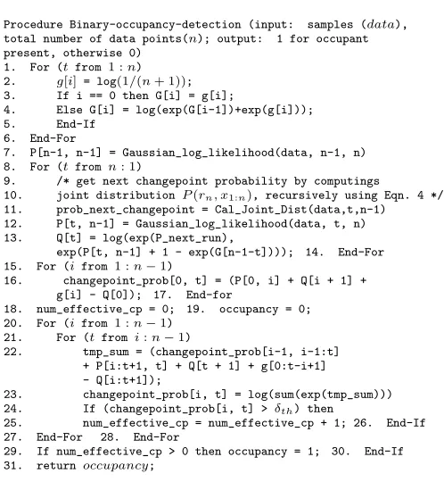
that sequence. Fig. 4 presents the changepoints and their probabilities which are being detected successfully in our proposed locomotive sensing model using smartphone’s ac-celerometer sensor. We filter those changepoints based on
empirically determined threshold probability (δth) and infer
presence of the occupants based on the admitted change-point sequence. We also count the number of changechange-points in the the data sequence which indicates movement score that represents how frequent a person moves. The overall algorithm has been summarized in Fig. 5.
0 5 10 15 20 25 30
0 500 1000 1500 2000
Magn
itu
de
No of Samples
0 0.1 0.2 0.3 0.4 0.5 0.6 0.7 0.8 0.9 1
0 500 1000 1500 2000
Pr
obab
ilities
No of Samples
Figure 4: Magnitude of accelerometer signal (Left) and change-points with probabilities of that signal (Right) due to a person’s random movement patterns
Procedure Binary-occupancy-detection (input: samples (data), total number of data points(n); output: 1 for occupant present, otherwise 0)
1. For (tfrom 1 :n)
2. g[i] = log(1/(n+ 1));
3. If i == 0 then G[i] = g[i];
4. Else G[i] = log(exp(G[i-1])+exp(g[i]));
5. End-If
6. End-For
7. P[n-1, n-1] = Gaussian_log_likelihood(data, n-1, n)
8. For (tfrom n: 1)
9. /* get next changepoint probability by computings
10. joint distribution P(rn, x1:n), recursively using Eqn. 4 */
11. prob_next_changepoint = Cal_Joint_Dist(data,t,n-1)
12. P[t, n-1] = Gaussian_log_likelihood(data, t, n)
13. Q[t] = log(exp(P_next_run),
exp(P[t, n-1] + 1 - exp(G[n-1-t]))); 14. End-For
15. For (ifrom 1 :n−1)
16. changepoint_prob[0, t] = (P[0, i] + Q[i + 1] +
g[i] - Q[0]); 17. End-for
18. num_effective_cp = 0; 19. occupancy = 0;
20. For (ifrom 1 :n−1)
21. For (tfrom i:n−1)
22. tmp_sum = (changepoint_prob[i-1, i-1:t]
+ P[i:t+1, t] + Q[t + 1] + g[0:t-i+1] - Q[i:t+1]);
23. changepoint_prob[i, t] = log(sum(exp(tmp_sum)))
24. If (changepoint_prob[i, t] >δth) then
25. num_effective_cp = num_effective_cp + 1; 26. End-If
27. End-For 28. End-For
29. If num_effective_cp > 0 then occupancy = 1; 30. End-If
31. return occupancy;
Figure 5: Binary Occupancy Detection Algorithm
4.3
Location Estimation
0 20 40 60 80 100 120
0 100 200 300 400 500 600
M
agn
e
tic
Fi
e
ld
(
u
T
)
Distance in Centimeter (cm)
Magnetic Signature containing Electrical Equipment
Pillar 1 Pillar 2 Pillar 3
Elevator
Figure 6: Magnetic signa-ture variation for different equip-ments.
0 20 40 60 80 100 120 140 160 180
1 11 21 31 41 51
Magn
itu
de (m
ic
ro T)
Time (s)
Room Level Magnitude Variation along Time
Room 461 Room 415
Figure 7: Magnetic signature variation along time for two rooms.
0 0.2 0.4 0.6 0.8 1 1.2
1 16 31 4661 76 91
N
or
m
aliz
ed
Magn
itu
de
Number of Samples
Normalized Magnitude of different rooms
Room 461 Room 411 Room 415
Figure 8: Normalized magni-tude of magnetometer for differ-ent rooms
0 0.2 0.4 0.6 0.8 1 1.2
1 10 19 28 37 46 55 64 73 82 91100
Ma
gn
itu
de
Number of samples Subject I Subject II
Figure 9: Normalized magni-tude of room for different sub-jects
near pillars, elevators etc., because pillars and elevators emit high magnetic fields. Magnetic fields produced by pillars are different for each floor because of their varying intensity level. This density characteristics guide with localization be-cause each floor is independent in structure and height with other levels, from which it is also probable to infer floor
level location. From this empirical observations, we
con-clude that each room has its unique magnetic fingerprint. We analyze different rooms data at University’s Informa-tion Technology and Engineering (ITE) building for three months. Fig. 7 represents this analysis which depicts each room specific magnetic fingerprint helping to create a coarse localization model for pinpointing the semantic location of gatherings at zone/room level.
We also note that this magnetic signal differs not only for different indoor environment but also for phone’s place-ment. This distraction has been optimized in two different
ways –i)calibrating magnetic signals, andii)calculating
ab-solute magnitude. During our experimentation we observe that magnitude represents different fingerprints for separate indoor environment. Fig. 8 describes how normalized mag-nitude of different rooms varies upon total number of sam-ples. Performing this experimentation over several rooms helps establish the fact that each room represents a differ-ent magnitude which may form their own fingerprint. We consider magnitude of magnetometer because for different persons with distinct movement, it does not deviate much other than little variations. Fig. 9 represents these charac-teristics where magnetic signature has been collected from two different people in the same room, both signals delin-eates same shape and almost same magnitude.
From this empirical study, we conclude that by only mag-netic signature, it is difficult to estimate fine-grained indoor location in different indoor environments, for this reason we also consider mean, standard deviation and variance of dif-ferent axes. Based on those feature vectors we generate two sets of data: training and testing using cross-validation pro-cess. We use training set to learn indoor characteristics by using different machine learning models and later use the testing set to predict location. To estimate fine-grained se-mantic location, we use SVM, J48, Random Forest classi-fiers.
4.4
Crowdsourcing Magnetic Model
We propose to use collaborative sensing or crowdsourc-ing to ease our ground truth data collection and location mapping process. We have divided the area of interest in-side the ITE building as a grid of squared cells (details are provided in Section 5.2). We collected data from most
fre-quently visited grids without any major obstruction. While crowdsourcing the unique characteristics of grid location, it was difficult to choose the right representation of data as analogous magnetic signatures of different grids in different locations were prevalent. As a result it was deemed neces-sary to display a potential set of locations from which the crowd would finalize the association of a semantic label with a particular observed magnetic signature pattern. Consider-ing this we provide the floor information for a specific signa-ture pattern, such that our crowdsourcing model will enable the crowd to choose the appropriate semantic location or room from that specific floor. Nevertheless the search space remains large as the possibilities of multiple rooms with sim-ilar magnetic footprints in a floor are quite abundance. We propose a simple grid mapping crowdsourcing model which reduces the search space by mapping the magnetic signature pattern of point of occupancy with the existing patterns and sorts the rooms according to the similarity measurement. Our model takes the Manhattan distance and the squared deviation of magnetic magnitude as input parameters for the mapped grids and search the repository of existing signature patterns database.
Consider a set of cell values found from a test pattern
X = x1, x2, x3...xn. First we take x1 from X and try to
map this value with the cell values of existing patterns. We do not assume to have any prior idea regarding the organi-zation of the cells in the test pattern. For mapping
signa-ture values we consider the deviation of±2 which have been
determined empirically according to our experiments. The patterns which matches the similarity value of a cell, we add
them to our candidate set,Cand initialize an×ndistance
matrixM¯(i)and an×1 deviation matrixD¯(i)for each
can-didate ci. M¯(i) records the manhattan distances between
the mapped cells in a candidate patternCiandD¯(i) stores
the squared deviation between the mapped cell values. If we find similarities in multiple cell values in a single room sig-nature pattern, we consider them as individual candidate.
We take the next test pattern, x2, in next iteration and
do the similar operation likex1, but this time we consider
only the candidates inC. In this iteration, if the deviation
and distance matrix of a candidatecjdoes not get updated
then we discard it from the candidate set and reduce the search space. We recursively perform the same mapping for remaining grid values and compute the final matching
candi-date setCF with their corresponding distance and deviation
matrices.
At this stage, it is still possible to have a large number of
candidates inCF. To tighten the search space, next we
sort the candidates with respect to this value assuming that in an ideal conversational episode the participants remain in
close proximity. We calculateE(Ci) based on Eqn. 5.
E(ci) = m
X
p=1
Xk,p( n
X
r=1 ¯
M(i)
a,rD¯(i)r,b)p,l (5)
wherek= 1, l= 1, 1≤a≤n, andb= 1
After calculating the error measurements for each
candi-date, we sort CF and choose the first 10 candidates from
CF. We plot the magnetic signature pattern of these
candi-dates and the test pattern. The crowd now have to choose the signature pattern in which they find the test pattern. In our experiments there were some cases where we observed empty candidate set. In these cases, we selected the last it-eration’s candidate set which was not empty. We also asked the crowd, if they found match with multiple candidates then they have to choose the earliest signature pattern.
5.
SYSTEM IMPLEMENTATION AND
EVAL-UATION RESULTS
We now discuss the detailed implementation and evalua-tion of our model framework.
5.1
Tools and Resources
We used Google Nexus-5 with built in microphone and three axes accelerometer sensor for our experiments. Our
en-tire system comprises of two parts:i)sensing, andii)
classi-fication and clustering, first one was implemented on Nexus-5 and latter on the server. Application software was written in Java which utilizes Android Programming Interface (API) to sense microphone and accelerometer signals. Classifica-tion and clustering algorithms and our occupancy counting algorithm have been implemented on the server side using python.
5.2
Data Collection
Magnetic sensor signals are sensed through our android application and stored temporarily on mobile storage. We first collected magnetic data for training set, and subse-quently for the testing set. We divided the room space into
small regions each contains area 0.5×0.5 m2 and named
as cell. Thus each room forms grid containing cells. We collected data from each cell for 5 minutes both clockwise and counter clockwise direction to form the training set. We also maintain fixed height (approximately 4 feet from the floor) when collecting our ferromagnetic fingerprint be-cause it also depends on the height. Partial 3rd floor map is shown in Fig. 10. It shows sample data collection path of room number 305 where green line shows how the grid forms and red line shows the data collecting path in both direction along the grid. We use sampling rate 5Hz for magnetometer sensor data. We implemented the acoustic sensing and col-lected conversational data from different places at different times in natural settings. Conversational data have been collected and properly anonymized during the spontaneous lab conversation among the students (without making the occupants aware of it), lab meeting, and general discussions in the lobby/corridor in presence of a variety of surrounding noise levels. The demographic for our conversational data collection was 1-10 persons (with 5 females and 5 males) in age group of 18-50 years. The acoustic data were collected
at a mono sampling rate of 16kHz at 16bit pulse-code mod-ulation (PCM).
5.3
Privacy
One of the major concerns of smartphone based acoustic signal processing is privacy. This concern becomes more se-rious when smart-phone records the conversation data. Our counting algorithm determines the number of speakers in this environment in an anonymized manner. We used text file as cover in which our recorded audio is embedded. A secret key is induced for embedding and extraction process which is known by both the sender and the recipient. A steganographic function takes cover file as argument and
then embeds audio file and key to produce stego as
out-put which is sent to our server. A reverse steganographic
function on our server side takes stego file and key as
pa-rameter and produces audio file as output. There are differ-ent steganographic methods (i.e. LSB coding, parity coding, phase coding) but we used the simplest method, least signif-icant bit algorithm which replaces the least signifsignif-icant bits of some bytes in the cover file to hide a sequence of bytes
containing hidden data. To generate thestego file, the
algo-rithm first converts each character of the cover file into bit stream followed by converting the audio file into bit streams and finally replacing LSB bit of the cover file with the bit of the audio in the secret information. We also ensured that the size of the file was not changed during this encoding and it was suitable for any type of audio file formats.
5.4
Magnetic, Acoustic and Locomotive
Fea-ture Extraction
We discuss different features relevant to our acoustic, lo-comotive sensing and localization technique in this section.
Magnetic Features:For location detection we used only magnetometer sensor. Smartphones’ magnetic sensor pro-vide three axes values x, y and z axis. From these values we
calculated magnitude using m =px2+y2+z2. We
con-sidered only the resultant magnitude to mitigate variations of the readings resulting from smartphone’s different axes based on different positions. We also calculated mean, vari-ance, and standard deviation of each readings and combined those features to generate the feature vectors.
Acoustic Features: We generated two basic features which are used in the speaker identification - MFCC and
Pitch. Each feature has been described in details in the
following.i) MFCC is one of the most significant features
which is used for acoustic processing. We followed the fol-lowing steps to process it. 1. Take the Fourier transform of (a windowed excerpt of) a signal, 2. Map the powers of the spectrum obtained above onto the Mel scale using triangular overlapping windows, 3. Take the logs of the powers at each of the Mel frequencies, 4. Finally, take the discrete cosine transform of the list of Mel log powers. We excluded the first co-efficient of MFCC and then chose 20 coefficients as
fea-ture vectors.ii) Pitchis defined as the lowest frequency of a
periodic waveform. It is the discriminative feature between man and woman. Human voice pitch interval falls within the range of 50Hz to 450Hz [23]. We calculated pitch of different segments using YIN [22] algorithm. We used 32 msec hamming window with 50% overlap for computing the Pitch and MFCC feature.
Figure 10: Sample Magnetic data collection path
0 0.2 0.4 0.6 0.8 1 1.2
0 2 4 6 8 10 12
Binar
y
O
cc
up
an
cy
Sensor Number Prediction Ground Truth
Figure 11: Locomotive
Sensing-based Occupancy Count
0 0.2 0.4 0.6 0.8 1 1.2 1.4 1.6 1.8 2
10 15 20 25 30
Av
er
ag
e
Err
or
C
oun
t
Similarity Measure Threshold (degree)
Figure 12: Performance with different cosine measures
0 0.1 0.2 0.3 0.4 0.5 0.6 0.7 0.8
2 3 4
Av
er
ag
e
Err
or
Coun
t Dis
tan
ce
Number of Speakers Table Pocket
Figure 13: Occupancy count over different phone positions
mitigate calibration.
5.5
Accuracy Metrics Definition
To evaluate and compare the performance of our location sensitive occupancy model, we first define the following
met-rics.i)Occupancy Metric:We computed the average
er-ror count as the normalized predicted occupancy metric
rep-resented by |ECN−AC|, where EC, AC, N respectively denote
the estimated people count, actual people count and num-ber of samples respectively. We presented only the absolute value in order to avoid any positive or negative contribution. ii) Location Metric: For evaluating location
measure-ment we consider the following metrics. Average
Preci-sion (T PT P+F P), Average Recall T PT P+F N, Average F-1 Score
(2×P recisionP recision+×RecallRecall), where TP, FP, TN and FN are the number of instances of true positive, false positive, true
neg-ative and false negneg-ative respectively. iii) Location
Pre-diction Error: It is defined as the mean absolute error be-tween predicted and actual value of the estimated variable.
This error is expressed as Mean Absolute Error =1
n
Pn
i=1 |
(fi−yi) |, where fi is the prediction andyi is the actual
value.
5.6
Occupancy Counting Results
We evaluated our opportunistic occupancy counting
al-gorithm in four scenarios. i)No conversation among
occu-pants,ii)All occupants are conversing in a single clique,iii)
Oc-cupants are conversing in multiple cliques, and iv) Mixed
conversing and non-conversing occupants.
For the first scenario, when no occupants are involved in a conversation we used the accelerometer to count the oc-cupancy. Each accelerometer sensor provides binary occu-pancy indication based on our change point detection al-gorithm as discussed in section 4.2 which computes the to-tal number of people present in the environment. Fig. 11 shows the total number of people successfully counted using our locomotive sensing model. We note that our locomotive sensing model achieves 80% accuracy (8 out of 10 people) in predicting occupancy when most of the users carry their smartphones with them.
Our opportunistic sensing system plays a critical role when all occupants have been conversing in a single clique. Our system helps to activate a single microphone for occupancy counting and deactivate all other microphones and accelerom-eter sensors based on the server’s feedback (details are omit-ted due to space constraints). Fig. 12 depicts the effect of cosine distant similarity measures on our occupancy count-ing algorithm as shown in Fig 3. We noticed that similar-ity distance angle measures (in degree) play a pivotal role on reducing the error count of occupancy inference. In our
experiments with 3 people conversing, we found that 15 de-gree similarity measure threshold is an appropriate choice for consideration to reduce the error count for our proposed adaptive people counting algorithm.
We also have run experiments in an uncontrolled environ-ment (completely in a natural setting) without imposing any restrictions on smartphones relative positions and distances from each other or from the server. Fig. 13 reports the
av-erage error count distance ≈ 0.5 with respect to different
positions of the phone. It is noted that when smartphone is placed on the table and two persons speak the error count becomes zero, but when three persons start speaking, error count tends to become slightly higher due to the ambient noise and overlapped conversation.
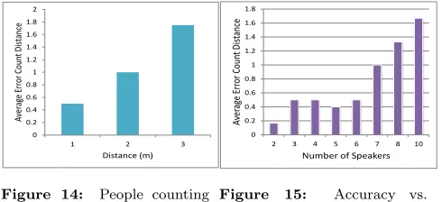
Fig. 14 depicts that error count increases as single clique leader’s distance from other occupants increases. We note that for a 3 meter distance error count becomes close to two which confirms that even for a large internal distance sepa-ration among the conversing occupants our acoustic sensing model performs quite well.
0 0.2 0.4 0.6 0.8 1 1.2 1.4 1.6 1.8 2
1 2 3
Av
er
ag
e
Err
or
Coun
t Dis
tan
ce
Distance (m)
Figure 14: People counting vs. phone distance
0 0.2 0.4 0.6 0.8 1 1.2 1.4 1.6 1.8
2 3 4 5 6 7 8 10
Av
er
ag
e
Err
or
C
ou
nt
Dis
tan
ce
Number of Speakers
Figure 15: Accuracy vs. Number of People
Fig. 15 presents the performance of our people counting algorithm where users speak naturally with overlapped con-versations. It is observed that average error count is 0.1 for 2 people and 1.7 for 10 people when conversing together. Thus the overall average error count is 0.76 with number of users present varying from 2 to 10 establishes that our acoustic-based occupancy counting algorithm performs well even in a crowded environment.
0 1 2 3 4 5 6 7 8 9
Group1 Group2 Group3
People
Cou
nt
Groups Estimated Ground Truth
Figure 16: People Counting vs. Multiple Co-located Group of Speakers 0 2 4 6 8 10 12
0 2 4 6 8
N um ber of O cc up an ts Test Cases Acc. Estimated Count Acc. Ground Truth Acoustic Estimated Count Acoustic Ground Truth Combined Count Combined Ground Truth
Figure 17: Locomotive Aug-mented Acoustic Occupancy Count 0.7 0.75 0.8 0.85 0.9 0.95 1
Random Forest J48 SVM
Me tric Sc or es Classifiers
Average Precision Average Recall Average F1
Figure 18: Location estimation errors for different classifiers
0 0.005 0.01 0.015 0.02 0.025
Stationary Random Same Reverse
Mea n Ab so lu te Err or Different Trajectory Random Forest
Figure 19: Location estimation error vs different trajectories
and 3 women) and last group has 8 occupants (4 men and
4 women). We observe that the mean error count is≈1 for
even our group based acoustic sensing model which attests the promise of our occupancy detection model in different real life scenarios.
Number of Speakers Crowd++ (Error Count) Our model (Error Count)
2 0.5 0.167
4 2.33 0.5
6 2.5 0.83
Average 1.78 0.5
Table 1: Comparison (Av-erage Error Count) between Crowd++ and Our model
65 70 75 80 85 90
P1 P3 P5 P7 P9
(%) of correct label
A nn o tato r No
Figure 20: Results of our Magnetic Crowdsourcing model
In our last scenario, where some people speak and some people remain silent arise, we propose to utilize our hybrid locomotive cum acoustic sensing model to infer total num-ber of occupants. For example, consider a scenario where six persons are involved in conversation while four remain silent. For conversing population, we activate either a sin-gle microphone sensor if there is a sinsin-gle clique or multiple microphone sensors if there are multiple conversing cliques
as determined by our “Estimate Proximity” module
imple-mented on the server. We use mean error count estimation to infer the number of people conversing. To estimate the number of people who are not involved in that conversation, we utilize our locomotive sensing model which postulates binary occupancy using change point detection applied on the accelerometer’s signal and finally infers the total num-ber of silent people. Fig 17 plots overall occupancy counting performance based on our hybrid approach. For example, when there are ten people and 6 persons converse in a single clique and 4 persons remain silent, our acoustic sensing es-timates 5 people out of 6 and locomotive sensing eses-timates 4 people out of 4, resulting in total of predicting 9 people out of 10. We have compared the performance of our model with Crowd++ framework [6] for counting the number of people. Table 1 shows that the average error count distance for Crowd++ is 1.78 where as for our model it is 0.5, more than a three fold increase in accuracy for inferring the total number of people.
5.7
Location Estimation Results
Fig. 18 presents the location estimation error of an oc-cupancy gathering using different classifiers. The Random Forest classifiers perform best with an average precision, re-call and F1 score of 0.98.
We also validated our location model through different
test cases where we consideri)different trajectories,ii)
dif-ferent times of a day, andiii) different rooms with varying
number of occupants.
We conducted our experiments following different trajec-tories, like keeping mobile phone on the table, following the same or reverse directions when collecting data and finally, collecting data randomly for a room. We noted that these different movement patterns do not affect much in the per-formance of our occupancy gathering location determination model. Fig 19 shows errors for different movement patterns. We find that stationary pattern shows better accuracy while moving in the same direction gives higher error rate. Aver-age errors are close to 0.015, which is quite acceptable with a minor number of false positives or true negatives.
Fig. 21 depicts the varying nature of the magnetic signa-ture during the different times of a day. We observe that the location estimation of any gatherings is similar during the different times of a typical day. It shows error ranges approximately from 0.015 to 0.03 due to the global variation of weather and other magnetic factors making our model as time invariant. 0 0.005 0.01 0.015 0.02 0.025 0.03 0.035
Morning Noon Evening
Mean Ab so lut e Err or
Different Times of a Day Random Forest
Figure 21: Location estimator error during the different time of a typical day
0 0.005 0.01 0.015 0.02 0.025 0.03 0.035 0.04 0.045 0.05
461 415 321 110
Mean Ab so lut e Err or Different Rooms Subject I Subject II
Figure 22: Location estima-tion error in different rooms with different occupancy size
We also ran experiments for location sensing model with respect to different rooms at different floors in ITE build-ing with a different set and size of the occupants. From Fig. 22, we do observe that the mean absolute error ap-proximately varies in the range of 0.015 to 0.04 which has negligible effect on the performance of our location
sensi-tive occupancy determination model. We observed some
toolkit [27]. We implemented our mapping algorithm on the
server side and then used the functionactive interactor of
VW to interact with the users. We showed 10 magnetic sig-nature patterns and 1 test pattern to an user and asked him to choose the magnetic signature pattern in which he/she finds the test pattern. 10 participants participated in the crowdsourcing task and in Fig 20 we show the overall accu-racy for each participants when given 15 pattern matching tasks. Average accuracy of gaining correct annotation for
these 15 patterns is≈81% which is adequately high. Our
results indicate that the probability for getting noisy labels is very low and the crowd annotated data can be chosen as input to the classifier.
6.
DISCUSSION AND FUTURE WORK
In the current version of our work, we have assumed that people keep their smartphone in the pocket or in the hand which might not be ideal in some cases. In future our plan is to make our architecture more robust and independent of smartphones’ location. The performance of our counting al-gorithm does not get affected by TV or radio sounds as TV or radio follows different modulation techniques which make it easier for us to remove those external noises from resultant audio signal systems. We have used source separation where significant overlap between human conversation and TV oc-curs. In the current implementation, location mapping pro-cess is independent of the classification propro-cess. In future we plan to develop and integrate a combined mapping and classification model. We also plan to investigate fine-grained floor level location using smartphone barometric sensing. We plan to investigate more advanced opportunistic sens-ing model considersens-ing microphone, accelerometer and mag-netometer sensor participation not only based on a server-based architecture but also server-based on an inter-smartphone distributed collaborative sensing based approach.
7.
CONCLUSIONS
In this paper, we presented an innovative system to infer the number of people present in a specific semantic loca-tion which opportunistically exploit accelerometer and mi-crophone sensor of smartphone for people counting. We pro-posed an acoustic sensing based unsupervised clustering al-gorithm by addressing the underpinning challenges evolving from naturalistic overlapped and sequential conversation to infer the occupancy in an environment. We posit a change point detection based locomotive sensing model to infer the number of people in absence of any conversational episode. We implement an opportunistic context-aware client-server based architecture to leverage smartphones’ microphone, ac-celerometer and magnetometer sensors and combine our acous-tic sensing with locomotive and semanacous-tic location sensing model to better predict the location augmented occupancy
information. We have also demonstrated a novel
crowd-sourcing model for reducing the effort of collecting location information at zone/room level at large scale. Our experi-mental results hold promises in a variety of natural settings with an average error count distance of 0.76 in presence of 10 users. We believe this investigation holds promises and helps to open up many new research directions in this op-portunistic multi-modal sensing domain.
Acknowledgement
This work is supported partially by the NSF Award #1344990,
and ConstellationE2: Energy to Educate Grant.
8.
REFERENCES
[1] Lawrence Rabiner and Biing-Hwang Juang.Fundamentals of Speech Recognition. 1993.
[2] Tanzeem Choudhury and Alex Pentland. Sensing and modeling human networks using the sociometer.
[3] D.B. Jayagopi and et al. Modeling dominance in group conversations using nonverbal activity cues.Proc. of IEEE TASLP (2009).
[4] Hong Lu, A. J. Bernheim Brush, and et al. Speakersense: Energy efficient unobtrusive speaker identification on mobile phones. InProc. of PerCom (2011).
[5] Rijurekha Sen, Youngki Lee, and et al. Grumon: Fast and accurate group monitoring for heterogeneous urban spaces. In Proc. of SenSys (2014).
[6] Chenren Xu, Sugang Li, and et al. Crowd++: Unsupervised speaker count with smartphones. InProc. of UbiComp (2013). [7] Youngki Lee, Chulhong Min, and et al. Sociophone: Everyday
face-to-face interaction monitoring platform using multi-phone sensor fusion. InProc. of MobiSys (2013).
[8] Robert Tomastik and et al. Model-based real-time estimation of ˆA˘abuilding occupancy during emergency egress. InProc. of PED (2008).
[9] Ebenezer Hailemariam and et al. Real-time occupancy detection using decision trees with multiple sensor types. InIn Proc. of SimAUD (2011).
[10] Hong Lu, Wei Pan, and et al. Soundsense: Scalable sound sensing for people-centric applications on mobile phones. In Proc. of MobiSys (2009).
[11] R.E. Yantorno B.Y. Smolenski U.O. Ofoegbu, A.N. Iyer. A speaker count system for telephone conversations. InProc. of ISPACS (2006).
[12] A. N. Iyer, U. O. Ofoegbu, R. E. Yantorno, and B. Y. Smolenski. Blind Speaker Clustering. InProc. of IEEE ISPACS (2006).
[13] Alessio Agneessens, Igor Bisio, and et al. Speaker count application for smartphone platforms. InProc. of IEEE ISWPC (2010).
[14] He Wang, Souvik Sen, and et al. No need to war-drive: Unsupervised indoor localization. InProc. of MobiSys, (2012). [15] Jaewoo Chung, Matt Donahoe, Chris Schmandt, Ig-Jae Kim,
Pedram Razavai, and Micaela Wiseman. Indoor location sensing using geo-magnetism. InProc. of MobiSys (2011). [16] K.P. Subbu, B. Gozick, and R. Dantu. Indoor localization
through dynamic time warping. InProc. of SMC (2011). [17] Indooratlas.https://www.indooratlas.com/.
[18] Luis A Castro, Jes´us Favela, and et al. Collaborative opportunistic sensing with mobile phones. InProc. of UbiComp (2014).
[19] Jitendra Ajmera, I McCowan, and H. Bourlard. Robust speaker change detection.Proc. of IEEE Signal Processing Letters (2004).
[20] Daben Liu and Francis Kubala. Fast speaker change detection for broadcast news transcription and indexing. InProc. of EuroSpeech (2009).
[21] Lie Lu and Hong-Jiang Zhang. Real-time unsupervised speaker change detection. InProc. of IEEE Pattern Recognition (2002).
[22] Alain de Cheveign´eb and Hideki Kawahara. Yin, a fundamental frequency estimator for speech and music.J. Acoust. Soc. Am (2002).
[23] Ronald J Baken and Robert F Orlikoff.Clinical measurement of speech and voice. Cengage Learning (2000).
[24] Paul Fearnhead. Exact and efficient bayesian inference for multiple changepoint problems. InProc. of Statistics and computing (2006).
[25] Xiang Xuan and Kevin Murphy. Modeling changing dependency structure in multivariate time series. InProc. of ICML (2007). [26] Kevin Murphy Xuan Xiang. Modeling changing dependency