Mobility Patterns Mining Algorithms with Fast Speed
Giang Minh Duc
1,*,
Le Manh
2and
Do Hong Tuan
31
HCM City University of Technology, HCM City, Vietnam
2
Van Hien University, HCM City, Vietnam
3
HCM City University of Technology, HCM City, Vietnam
Abstract
In recent years, mobile networks and its applications are developing rapidly.
Therefore, the issue to ensure quality of service (QoS) is a key issue for the service
providers. The movement prediction of Mobile Users (MUs) is an important problem in
cellular communication networks. The movement prediction applications of MUs
include automatic bandwidth adjustment, smart handover, location-based services,…
In this work, we propose two new algorithms named the Find_UMP_1 algorithm and
the Find_UMP_2 algorithm for mining the next movements of the mobile users. In the
Find_UMP_1 algorithm, we make to reduce the complexity of the traditional
UMPMining algorithm. In the Find_UMP_2 algorithm, we perform to reduce the
number of transactions of the User Actual Paths (UAPs) database. The results of our
experiments show that our proposed algorithms outperform the traditional
UMPMining algorithm in terms of the execution time. In addition, we also propose the
UMP_Online algorithm in order to reduce the execution time as adding new data. The
benefit of applying the UMP_Online algorithm is that the system can run online in real
time. Therefore, we can perform the applications effectively.
Keywords: mob ility patterns, mob ility rules, cellular communication networks, data mining, mob ility prediction.
Received on 14 August 2015, accepted on 27 September 2015, published on 05 November 2015
Copyright © 2015 Giang Minh Duc et al., licensed to EAI. This is an open access article distributed under the terms of the Creative Commons Attribution licence (http://creativecommons.org/licenses/by/3.0/), which permits unlimited use, distribution and reproduction in any medium so long as the original work is properly cited.
doi: 10.4108/eai.5-11-2015.150603
Corresponding author. Email: [email protected]
1. Introduction
Currently, due to the rapid development of mobile communication networks, many people use personal mobile devices to search for information on the Internet. Almost everyone has a mobile device as cell phone, personal digital assistant (PDA) or notebook. In addition, many people search for information while traveling all over the world. At about 6.8 billion mobile phones are used around the world in 2013 at the rate of 96, 97% of the world population [1].
Therefore, the propose problem is how to ensure quality of mobile services.
HLR is a database which long-term storage of information of MUs. The movement history of MUs is extracted from the log files and it is stored in the HLR of the MSC. The historical data is used to predict the mobility of MUs.
Due to the properties of the cellular communication networks are mobility, disconnection, long time delay, hand-off, bandwidth continuously changing... so there were some recent researches, which applied the traditional User Mobility Pattern (UMP) Mining algorithm ([7], [8], [9], [10]) to overcome these problems. However, the UMP Mining algorithm has a long execution time, running offline. Therefore, the above applications are reduced effectiveness.
In particular, our main contributions can be summarized as follows:
Our proposed algorithms make increased running speed of the traditional UMP Mining algorithm in two ways. (1) We perform to reduce the complexity of the traditional UMP mining algorithm. (2) We reduce a number of transactions when movements mining of MUs.
We propose UMP_online algorithm to avoid scanning of full database again. This algorithm executes to mine the new dataset (new transactions are added to the database). Therefore, the mobile service providers (MSPs) can supply their applications more efficiently. The results of our experiments show that:
-Execution time of the first improvement (Find_UMP_1 algorithm) reduces more than 25% compared with the traditional UMPMining algorithm.
-Execution time of the second improvement (Find_UMP_2 algorithm) reduces more than 75% compared with the traditional UMPMining algorithm. -The third improvement (UMP_Online algorithm) has an
execution time down about 57.94% compared with the Find_UMP_2 algorithm.
The rest of our paper is organized as follows. In section 2, we present related work. In section 3, our proposed scheme is explained. Finally, we present the experimental results in Section 4 and conclude our work in section 5.
2. Related work
Problem mining sequential patterns mentioned in [6], [7], [8], [9]. The algorithm in [6] applied Apriori algorithm in grid computing and does not take into the topology of the network while creating the candidate patterns. In [14], Mira H. Gohil and S. V. Patel compared different methods of the next location prediction.
The UMPMining algorithm in [7] predicts the next location of mobile users using data mining techniques . In [7], Yavas et al presented an AprioriAll based sequential pattern mining algorithm to find the frequent sequ ences and to predict the next location of the user. They compared their algorithm’s results with Mobility Prediction based on Transition Matrix (TM). In [10], Byungjin Jeong applied the
UMPMining algorithm to perform the decision smart handover for the purpose of reducing the number of unnecessary handover in architecture Macro / Femto -cell networks.
In [11] and [12], the authors also applied the UMPMining algorithm for location-based services (LBSs) in the cellular communication networks. In [11], Abo-Zahhad et al. presented LBSs as emergency, safety, traffic management, and public information applications. In [12], Lu et al., presented to find segmenting time intervals where similar mobile characteristics exist.
The above works apply the traditional UMPMining algorithm to enhance quality of services. Our algorithms improve the traditional UMP algorithm to further enhance the quality of services.
3. Proposed scheme
Before giving our proposed algorithms, we present the traditional UMP Mining algorithm in [7] and calculate its complexity in subsection A as follows.
3.1 The traditional UMPMining algorithm:
Suppose that User Actual Paths (UAPs) have a form as follows: C = {c1, c2... cn}. Each ck denotes the ID number of
the cell kth in coverage area.
For example, we have the coverage map simulated as follows:
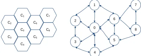
Figure 1. The simulation of the cellular network and graph G
The data of UAPs as follows:
Table 1. Paths of mobile users
UAP ID UAPs
1 {5,6,0,4}
2 {3,4,5,0}
3 {1,2,3,4,0,5}
4 {3,2,0}
C4
C8
C7
C5
C6
C1
C2
C0
C3
2
3
8 7
0 5 6 1
G is called a directed graph corresponds to cells in the mobile coverage area. Each cell of the G is a node as Fig. 1. If there are two cells that called A, B neighboring each other (a common border) in the mobile coverage area, they have a directed and unweighted edge from A to B and from B to A.
Definition 1:
Suppose that there are two UAPs, A = {a1, a2,... an} and
B = {b1, b2... bm}. B is a substring of A, if exist: 1 ≤ i1 <... <
im ≤ n, bk = aik, k, and 1 ≤ k ≤ m.
In addition, B is a substring of A, if all cells of B exist in A (not need sequent in A).
For example, in Figure 1, suppose that A = {c4, c0, c6, c7,
c8, c5) and B = {c6, c8} is the length-2 sequence of A. In
addition, The UAP B is contained by the UAP A.
The UMPMining algorithm is a sequence pattern mining algorithm which applied in the movement predict of the cellular networks ([7], [8], [9], [10], [11], [12]).
UMPMining algorithm
Input: UAPs of database D, min_supp, graph G Output: L (UMPs)
1. C1 the length-1 patterns
2. k = 1
3. L = // initially the set is empty
4. while Ck
5. for each (UAP a D) do
6. S = {s s Ck and s is subsequence of a}
7. for each s S do
8. s.count = s.count + s.suppInc
9. endfor
10. endfor
11. Lk = {s s Ck, s.count min_supp }
12. L = L Lk
13. Ck+1 Cand_Gen (Lk, G), c Ck+1,, c.count = 0
14. k = k + 1
15. endwhile
16. return L
At line 13, the Cand_Gen() function is written as follows:
Cand_Gen algorithm Input: Lk; G
Output: Candidates (Ck+1)
1. Candidates = //initially the candidates set is empty
2. for each L = (l1, l2, …, lk), L Lk do
3. N+ = {v lk v }
4. for each v N+ (lk) do
5. C’ = (l1, l2, …, lk, v)
6. Candidates Candidates C’
7. endfor
8. endfor
9. return Candidates
For UMPMining algorithm, from line 5 to line 10 (finding support of Cn) is rewritten as follows:
Find_suppor t_ UMP(Sk) Input: database D
Output: SP(Sk) (support of Sk)
1. for each (UAP a D) do //scan all database D 2. for (i = 1; i |a|; i++) do //|a|: length of sequence a 3. Find position (s1, s2, …, sk) Sk in sequence a
4. Find Sk.count
5. endfor
6. endfor
7. return SP(Sk)
The complexity of the Find_support_UMP function: For the loop at line 1: the complexity is O(m), where m
= |D|
For the second loop (line 2): the complexity is O(n), where n = | a |: the average length of string a D.
Thus, the complexity of this algorithm is: O(mn).3.2. Find_UMP_1 algorithm
We map the UAPs database (D) to the Mdd Mobility
Matrix (definition 6).
Steps as follows:
Definition 2: Data Mining Context
Let O be a non-empty limited set of transactions (UAP ID) and I be a non-empty limited set of cells, R be a two subject relation between O and I such that o O and i I, (o,i) R transaction o contains cell ith. The data mining
context is the triple (O, I, R).
Definition 3: Data Mining Context Matrix
Give a mobile user’s paths table includes two properties that are UAP_ID (code of a transaction) and UAP (path of a mobile user through the cells of the mobile coverage map). Call O is a set of transactions. I is a set of cells and R is a two subject relation between O and I, R OI, where (o, i) R if and only if transaction o is contained cell ith.
Definition 4: Galois Connection
Give a data mining context (O, I, R), where two functions and , they are defined as follows: P(I) P(O) and P(O) P(I):
Give S I, (S) = {o O i S, (o,i) R} Give X O, (X) = {i I o X, (o,i) R}
Where P(X) is a set of subsets of X. A pair of function (,) is defined in such that is called Galois Connection.
(S) value denotes a set of transactions that have common all cells in S. (X) The value denotes a set of cells that have in all transactions of X.
Property 1: a pair of function (, ) has properties as follows:
1.1 Where S1, S2 P(I), S1 S2(S2) (S1)
1.2 Where X1, X2 P(O), X1 X2 (X2) (X1)
1.3 S ((S)) and X ((X))
1.4 (((X))) = (X) and (((S))) = (S)
Definition 5: the frequent set
Give a data mining context (O, I, R), and S I, the frequency level of S is defined as the ratio of the number of transactions to all of the transactions . The frequent of S is called the support of S (SP(S)) and it is computed as follows:
Where . is the length of the set.
Give S I and min_supp is a minimum support threshold, S is a support set by the min_supp threshold if and only if SP(S) min_supp.
FS (O, I, R, min_supp):is the set of the support subsets satisfy the min_supp threshold or FS (O, I, R, min_supp) = {S P (I) SP(S) min_supp}
Clause 1:
Give S FS(O, I, R, min_supp), if T S, then T FS(O, I, R, min_supp)
Demonstration: due to T S, according to property (1.1) of the Galois Connection of a pair of function (, ), we have (S) (T), therefore min_supp SP(S) SP(T) T FS(O,I,R,min_supp).
Clause 2:
Give T FS(O, I, R, min_supp), if T S, then S FS(O, I, R, min_supp).
Demonstration: due to T S, according to property (1.1) of the Galois Connection of a pair of function (, ), we have (S) (T), therefore SP(S) ≤ SP(T) < min_supp S FS(O,I,R,min_supp).
Definition 6: Mdd mobility Matrix
The Mdd mobility matrix is similar to the binary matrix
as definition 3, but it is added as follows: each M [Om, in] is
a location of a mobile user traveling in mobile network (Table 2).
Column in: code of a cell in mobile network.
Row om: the actual paths of a mobile user.
We exchange data from the table 1 to table 2 as follows:
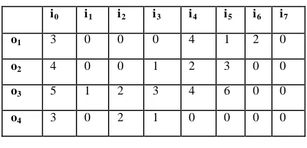
Table 2. Mobility matrix of mobile users
i0 i1 i2 i3 i4 i5 i6 i7
o1 3 0 0 0 4 1 2 0
o2 4 0 0 1 2 3 0 0
o3 5 1 2 3 4 6 0 0
o4 3 0 2 1 0 0 0 0
For example, in table 2, mobile user 2 (UAP ID = 2) moves between the cells as follows:
Figure 2. Mobility of UAP ID = 2
Therefore, the path o2 performs the following: o2 = (4, 0, 0,
1, 2, 3, 0, 0)
The following is a new algorithm to find UMPs from the mobility matrix Mdd:
Find_UMP_1 algorithm Input: min_supp, Mdd, G
Output: L
1. L = // initially the large patterns set is empty 2. L1 ← Find_L1 //generate L1 from Find_L1 function
3. for (k=2; Lk-1; k++) do
4. Lk ← Find_Lk(Lk-1) //generate Lk from Lk-1
5. L = L Lk
6. endfor
7.
return LAt line 2, we have Find_L1() function as follows:
Find_L1 algorithm
Input: (O, I, R), min_supp, Mdd, G
Output: L1.
1. L1 =
2. for each (i I and j field of Mdd) //i: cell ID and it
is also a column of Mdd
3. S={s | s Mdd and sij 0}
4. for each s S
5. s.count = s.count + 1
6. endfor
7. endfor
8. L = {s | s C1, s.count ≥ min_supp}
9. L1 = L1 L
10. return L1
At line 4 of Find_UMP_1 algorithm, we have a function finds Lk from Lk-1 as follows:
Find_Lk(Lk-1) algorithm Input: Lk-1, G, Mdd
Output: Lk
1. Lk =
2. for (each X Lk-1) do
3. for (each Y Lk-1 and X Y) do
4. S = X Y
5. S = {s1,s2,…,sk-1,sk} //sk: a set of cells be linked
to sk-1 of G
6. if (|S| = k and SP(S) ≥ min_supp) then 7. Lk = Lk {S}
8. endif
9. endfor
10. endfor
11. return Lk
At line 6 of Find_Lk(), we have a function finds the support
of Sk as follows:
Find_suppor t(Sk) algorithm Input: Sk, Mdd
Output: SP(Sk)
1. for each o Mdd do //scan all Mdd
2. Find location (s1,s2,…,sk) Sk of o Mdd
3. Find Sk.count
4. endfor
5. return SP(Sk)
The complexity of the Find_support() algorithm: - For the loop at line 1: the complexity is O(m), where m
= |O|: the total number of records of Mdd
- Thus, the complexity of the algorithm is: O(m).
The complexity of the Find_support algorithm is reduced n times (reduce of one loop) compared to UMPMining algorithm.
3.3. Find_UMP_2 algorithm
The Find_UMP_2 algorithm is similar to the Find_UMP_1 algorithm, they differ from the function to find the support, as follows:
Decreasing the number of transactions: According to the clause 2, we have:
T FS(O, I, R, min_supp), if T S, then S FS(O, I, R, min_supp).
Find_Supp_2(Sk) algorithm Input: Mdd, Sk, min_supp, G
Output: SP(Sk)
1. Dem_dong = 1 2. ifSk = 2 then
//scan all rows of Mdd (on Mdd)
3. for (i = 1; i ≤ O; i++) do
4. if (Sk O and (s1,s2,…,sk) have in order of O) then
5. Store_Array ← save variable i
6. Store_Array ← count the number of rows
7. endif
8. endfor
9. else //Sk > 2
10. Sk-1 ← Sk
11. |OR| ← Store_Array //|OR|: the number of rows
contains Sk-1
12. for (i = 1; i ≤ |OR|; i++) //|OR| < O
13. if (Sk OR and (s1,s2,…,sk) have in order of OR)
then
14. Store_Array ← save variable i
15. Store_Array ← count the number of rows
16. endif
17. endfor
18. endif
19. SP(Sk) ← Find support
20. if SP(Sk) ≥ min_supp then
21. Store_Array ← Temp_Array
22. endif
Remarks:
When |Sk| = 1, the method calculating the support of the
Find_support (Sk) and the Find_support_2 (Sk)
algorithm is the same, so the execution time of the two algorithms are equal (as shown table 6).
When |Sk| = 2, the method calculating the support of the
Find_support_2 (Sk) algorithm is added line 4 7, 20
22 with the following meanings:
- If SP(Sk) ≥ min_supp, we save these rows to the
Store_Array including the number of satisfied rows and Sk.supp.
Our purpose reduces the number of the loop time as finding Sk+1. According to clause 2, we show that: if Sk
FS(O, I, R, min_supp) and Sk Sk+1, then Sk+1
FS(O, I, R, min_supp). For example, if Sk = {3, 2} and
SP(Sk) = 1 ≤ min_supp = 1.33, then Sk+1 = {3, 2, 1} ≤
min_supp.
- This algorithm was executed for an actual database as follows:
Input data UAPs have the number of paths as : 56 198 (all rows of matrix Mdd: |O| = 56 198).
The number of BTSs is 351 (The number of fields of matrix Mdd: | I | = 351).
When |Sk| ≥ 2:
- At line 10 11: get the number of rows contained Sk-1
be OR to reduce the number of the loop.
- At line 12 17: instead of scanning of full database, we just execute the OR loop times.
3.4. UMP_Online algorithm
In this section, we develop the incremental algorithms to find the large sets from the mobile database. The proposed algorithm is named UMP_Online. In order to avoid s canning of full database again, this algorithm executes to mine the new dataset (new transactions are added to the database).
The purpose of this algorithm is to reduce the execution time of mining the MUs movements. Therefore, MSPs can supply their applications more efficiently.
Here is the UMP_Online algorithm:
UMP_Online algorithm
Input: New candidate sets have length-i: Cinew
Old candidate sets have length-i: Ci
Old large sets have length-i: Li; min_supp
Output: New large set: L
1. for each (c Cinew)
2. if c Ci then
3. supptotal = s.supp + c.supp //s Ci và s = c
4. s.supp = supptotal
5. if supptotal >= min_supp then 6. if c Lithen
7. l.supp = supptotal //l Li; l = c = s
8. else // c Li
9. Li = Li c
10. Find_Lk()
11. endif
12. else // c Ci
13. Ci = Ci c
14. if (c.supp >= min_supp) then 15. Li = Li c
16. Find_Lk()
17. endif
18. endif
19. endif
20. endfor
21. return L
The old result table is the candidate sets Ci and the large
patterns Li (Ci, Li are found as running the Find_UMP_2
algorithm). This algorithm uses the previous results and takes update to the mobility patterns as follows:
- Finding the candidate patterns (Cinew) from the new data
set.
- The support value is calculated for each sequence c Cinew,if the min_supp value is satisfied.
- Update the candidate patterns (if c.supp ≥ min_supp) to the old candidate patterns (Ci, Li).
- Returning the new large set: L.
L finding enough all Li. When Li gives rise (line 9 and 15),
the algorithm calls the Find_Lk() function (line 10 and 16).
Theorem 1: the Find_Lk algorithm ensures to find
enough all keys.
Using the inductive method to prove the Find_Lk
algorithm that ensures to find all keys.
First, L1 is true because L1 = {SP(I) | SP(S) ≥ minsupp
|S| = 1}
Suppose that Lk-1 is true, we should prove the Find_Lk
algorithm creates Lk true. That is Lk contained all large sets
S, so that | S | = k.
Indeed, due to set X Fk-1 and Y Fk-1, so |X| = |Y| = k-1.
In addition to wanting S = X Y is a candidate, then |S| = k (line 6 of the Find_Lk algorithm). According to clause 2, the
set S Lk must be the large sets Lk candidates should be
created from Lk-1 (line 2, line 3 of the Find_Lk function).
3.5. Finding the mobility rules
According to the results from the data mining phase (UAPs UMPs); the mobility patterns of mobile users (UMPs) were founded. In this section, we will find the mobility rules from UMPs.
Example: we have a form UMP is (3, 4, 5). The mobility rules as follows:
(3) (4, 5)
(3, 4) (5)
Suppose that we have the UMP L = {i1, i2,… ik}, where
k > 1. All mobility rules are generated from the pattern as follows:
{i1} -> {i2,…, ik}
{i1, i2} -> {i3,…, ik}
…
{ i1, i2,…, ik-1} -> { ik }
Give the mobility rule R is: (i1, i2,…, im-1) (im, im+1,…,
ik), the confidence value is calculated as follows:
Confidence( R) =
count m
i i i
count
). 1 ,..., 2 , 1 (
. ) k i , , 2 i , 1 (i
100
By using UMPs, all mobility rules are generated and the confidence value is also calculated. Rules (if confidence min_conf) will be selected.
.Finding the mobility rules:
We have the rules generation algorithm as follows:
Gen_Rules algorithm
Input: Minimum confidence value: min_conf User mobility patterns: UMPs
Output: Set of mobility rules: R
1. for all L UMPs, L = (i1, i2, . . . , ik), where k > 1 do
2. for all m from 1 to k - 1 do 3. //get all the mobility rules
4. head =(i1, i2, . . . , im-1)
5. tail =(im, im+1, . . . , ik)
6. rule = head → tail
7. //calculate the confidence value of the rule 8. rule.conf = (L.count/head.count) * 100
9. if rule.conf ≥ min_conf then
10. R = R rule
11. end if
12. end for
13. end for
14. return R
At line 4, the head is the part of the rule before the arrow. At line 5, the tail is the part of the rule after the arrow (rule = head tail).
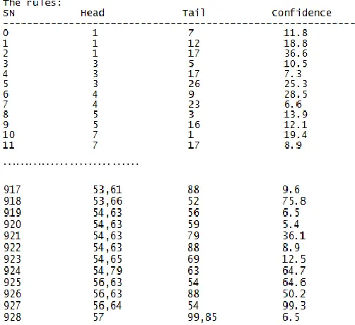
After running the Gen_Rules algorithm, we have the results table from actual data as follows (min_conf = 5%):
Table 3. The rules result
………
. The movement prediction of mobile users:
From the above rules results (set of mobility rules R), we find out the set of predicted cells as follows:
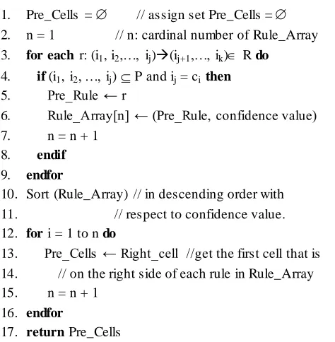
Pre_Mov algorithm
Input: Current movement of the user: P = (c1, c2, …, ci)
Set of mobility rules: R.
Output: Set of predicted cells: Pre_Cells.
1. Pre_Cells = // assign set Pre_Cells = 2. n = 1 // n: cardinal number of Rule_Array 3. for each r: (i1, i2,…, ij)(ij+1,…, ik) R do
4. if (i1, i2, …, ij) P and ij = ci then
5. Pre_Rule ← r
6. Rule_Array[n] ← (Pre_Rule, confidence value)
7. n = n + 1
8. endif
9. endfor
10. Sort (Rule_Array) // in descending order with 11. // respect to confidence value. 12. for i = 1 to n do
13. Pre_Cells ← Right_cell //get the first cell that is 14. // on the right side of each rule in Rule_Array 15. n = n + 1
16. endfor
17. return Pre_Cells
In this part, the next movement of user is predicted. Suppose that the movement of a user (up to now) is P = (64, 56, 63). Current this user is being cell 63 of the coverage region. The algorithm finds out the rules as follows: (56, 63) (54) and (56, 63) (88) (line 925 and 926 of Table 3). The set of predicted cells is {54, 88} (both cell 54 and cell 88 are selected). The cell 54 is selected first because it has the confidence value more than the confidence value of the cell 88 (64.6 and 50.2).
4. The experimental results
In this section, we investigate the performance of our Find_UMP_1, Find_UMP_2, UMP_Online algorithms and compare them with the performance of the traditional UMPMining algorithm in terms of the execution time.
Our experimental environments are given in Table 4. Training data set and Testing data set used form [13].
Training data set: the number of UAPs. Training data sets include three sets given in Table 5.
Table 4. Experimental environments
Name Parameter
Processor Intel Core i3-2330M, 2.20GHz
RAM 4 GB
Operating System 32-bit
Programming language
Microsoft Visual Studio 2005
Database management system
SQL Server 2005
Table 5. Training data sets
Name Number of transactions of MUs
Data set 1 56198
Data set 2 68787
Data set 3 34895
These datasets are the actual database of MUs. The database is transformed from the User ID to the integer n (n = 1, 2, 3,...) and they cannot be decoded to protect customer information.
- The testing dataset is UAPs; it is used to evaluate the accuracy of the users’ mobility prediction.
Testing data set contains 7207 transactions of MUs.
The number of BTS: 351.
4.1. Compare the execution time of the
algorithms: UMPMining, Find_UMP_1 and
Find_UMP_2
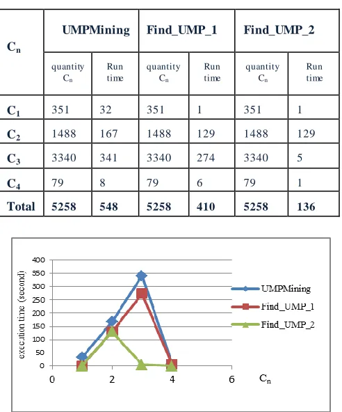
Table 6. The results of three algorithms
Figure 3. The execution time results of three algorithms
Figure 4. The execution time total of three algorithms
4.2. The experimental results when running
the UMP_Online algorithm
When not applying the algorithm UMP_Online:
Each update a new data set, we perform as follows:
- Database (total) = database (old) + database (new) - Running the Find_UMP_2 algorithm for database
(total).
When applying the algorithm UMP_Online:
We perform as follows:
- Get the old results (Cn, Ln).
- Running the UMP_Online algorithm for the new database and update the result with the old results new results.
To compare the results of the two methods above, we have the actual results as follows:
- Database (old): data set 1 (the number of records is 56 198).
- Database (new) data set 2 (the number of records is 68 787).
- Database (total): data set 1 + data set 2 (the number of records is 124 985)
- The execution time is 214 seconds.
When running UMP_Online algorithm, the execution time is 90 seconds (down 57.94%).
The same as above, we have:
- Database (old): data set 1 (DS1) + data set2 (DS2) (the number of records is 124 985)
- Database (new): data set 3 (the number of records is 34 895)
- Database (total): data set 1 (DS1) + data set 2 (DS2) + data set 3 (DS3) (the number of records is 159 880) - The execution time of the Find_UMP_2 algorithm is
284 seconds.
The execution time of the UMP_Online algorithm is 95 seconds (down 66.54%).
Figure 5. The execution time of two algorithms
4.3. The accuracy of the prediction:
- Recall: the number of correctly predicted cells / the total number of requests.
-
Precision: the number of correctly predicted cells / the total number of predictions made.
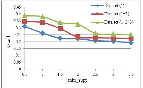
Changing of the recall values according to the min_supp values:
In Figure 6, if the min_supp value increases, then the recall value decreases. The reason is the increasing min_supp value will make the number of prediction rules
Cn
UMPMining Find_UMP_1 Find_UMP_2
quantity Cn
Run time
quantity Cn
Run time
quantity Cn
Run time
C1 351 32 351 1 351 1
C2 1488 167 1488 129 1488 129
C3 3340 341 3340 274 3340 5
C4 79 8 79 6 79 1
decreased. Therefore, the number of correctly predictions is decreased.
Figure 6 compares the recall value changes of three data sets.
When the size of the training set increases, the recall values also increase (because the number of prediction rules increases).
Figure 6. Changes of recall according to min_supp of three data sets
The precision of the prediction rules when ch anging the min_conf value:
Testing data set: 7207 records.
When changing the minimum confidence value (min_conf), the precision value changes as Figure 7.
In Figure 7, when the min_conf value increases, the precision value also increases. Because of high min_conf values, only the rules that have high confidence values are used for prediction.
Figure 7. Precision of the prediction rules
5. CONCLUSION
The mobility prediction of Mobile Users is one of the important issues in mobile computing sys tems. Applications of the MUs mobility prediction are adjusting bandwidth of the networks, the location-based services, smart handover, ... However, these applications require the execution time of the UMPMining algorithm as quickly as possible. In this work, we proposed Find_UMP_1 algorithm and the Find_UMP_2 algorithm to solve the time problem. The results of our experiments shown that our proposed algorithms outperform the traditional UMPMining algorithm in terms of the execution time.
In addition, we also propose the UMP_Online algorithm in order to reduce the execution time as adding new data. The benefits of applying this algorithm are that the system can run online in real time. Therefore, MSPs can perform the above applications effectively.
References
[1] “List of Countries by Number of Mobile Phones in Use,” Wikipedia, Gartner, 2010 .
[2] ETSI/GSM . Technical reports list.
http://webapp.etsi.org/key/key.asp? full list=y.
[3] ETSI/GSM . Home location register/visitor location register – report 11.31–32.
[4] Alex Cabanes (IBM Systems & Technology Group): IBM BladeCenter - Home Location Register (HLR). June 2007.
[5] HRL Look Up – Service M anual
(www.routomessaging.com).
[6] Cristian Aflori and M itica Craus. “Grid implementation of Apriori algorithm. Advances in engineering software”. Volume 38, Issue 5, 295-300, 2007.
[7] Gokhan Yavas, dimitrios Katsaros. Ozgur Ulssoy and Yannis manolopoulos. “A data mining approach for location prediction in mobile environments”. Data and Knowledge Engineering, 54, 121-146, 2005.
[8] M r. M ohammad Waseem, M rs. R.R.Shelke, Location Pattern M ining of Users in M obile Environment, International Journal of Electronics, Communication & Soft Computing Science and Engineering, 2013, ISSN: 2277-9477, Volume 2, Issue 9
[9] V. Chandra Shekhar Rao and P. Sammulal. Article: Survey on sequential pattern mining algorithms. International Journal of Computer Applications, 76(12):24–31, August 2013. Published by Foundation of Computer Science, New York, USA.
[11] M . Abo-Zahhad, Sabah M . Ahmed, M . M ourad, “ Services and Applications Based on Mobile User’s Location Detection and Prediction”, Int. J. Communications, Network and System Sciences, 2013, 6, 167-175.
[12] Lu, E. H.-C.; Tseng, V. S.; and Yu, P. S. 2011. “M ining cluster-based temporal mobile sequential patterns in location-based service environments”. IEEE Trans. Knowl. Data Eng. 23(6):914–927.
[13] http://msdn.microsoft.com/en-us/ library/ bb895173.aspx
(Training and Testing Data Sets – M SDN – M icrosoft). [14] M ira H. Gohil and S. V. Patel, “M obile Location Prophecy: