Forecast skill score assessment of a relocatable ocean prediction system, using a simplified objective analysis method

https://doi.org/10.5194/os-13-925-2017

© Author(s) 2017. This work is distributed under the Creative Commons Attribution 3.0 License.

Forecast skill score assessment of a relocatable ocean prediction

system, using a simplified objective analysis method

Reiner Onken

Helmholtz-Zentrum Geesthacht (HZG), Max-Planck-Straße 1, 21502 Geesthacht, Germany Correspondence to:Reiner Onken ([email protected])

Received: 5 May 2017 – Discussion started: 23 May 2017

Revised: 26 September 2017 – Accepted: 9 October 2017 – Published: 20 November 2017

Abstract. A relocatable ocean prediction system (ROPS) was employed to an observational data set which was col-lected in June 2014 in the waters to the west of Sardinia (western Mediterranean) in the framework of the REP14-MED experiment. The observational data, comprising more than 6000 temperature and salinity profiles from a fleet of underwater gliders and shipborne probes, were assimilated in the Regional Ocean Modeling System (ROMS), which is the heart of ROPS, and verified against independent observa-tions from ScanFish tows by means of the forecast skill score as defined by Murphy (1993). A simplified objective analy-sis (OA) method was utilised for assimilation, taking account of only those profiles which were located within a predeter-mined time window W. As a result of a sensitivity study, the highest skill score was obtained for a correlation length scaleC=12.5 km,W=24 h, andr=1, whereris the ratio between the error of the observations and the background er-ror, both for temperature and salinity. Additional ROPS runs showed that (i) the skill score of assimilation runs was mostly higher than the score of a control run without assimilation, (i) the skill score increased with increasing forecast range, and (iii) the skill score for temperature was higher than the score for salinity in the majority of cases. Further on, it is demon-strated that the vast number of observations can be managed by the applied OA method without data reduction, enabling timely operational forecasts even on a commercially avail-able personal computer or a laptop.

1 Introduction

A relocatable ocean prediction system (ROPS) is presented which enables rapid nowcasts and forecasts of ocean envi-ronmental parameters in limited regions. In this study, ROPS was implemented for the waters west of Sardinia (western Mediterranean Sea) within the framework of the REP14-MED experiment (Onken et al., 2014, 2018).

The major components of ocean operational systems are observations and ocean circulation models coupled with data assimilation systems, to combine the observations with dy-namics and issue nowcasts and forecasts which are deliv-ered to the customers. While systems on the global scale are utilised to provide estimates on large-scale circulation patterns and associated features, regional operational sys-tems are focused more on societally relevant oceanographic information for, e.g., search and rescue operations, pollu-tant dispersal, fishery management (Edwards et al., 2015), and military applications. Meanwhile, a number of real-time ocean operational systems are available, spanning the scales of ocean horizontal circulation patterns from global to coastal (Dombrowsky, 2011; Zhu, 2011).

on the Harvard Ocean Prediction System (HOPS; Robinson, 1999) may be considered as the pioneering work in this sub-ject. They became available since the late 1990s, and have been applied in various regional studies up to the present (De Dominics, 2014). Another line of research based on the Naval Coastal Ocean Model (NCOM; Martin, 2000) can be traced back to the first decade of the present century (Row-ley and Mask, 2014), and recently, Trotta et al. (2016) sented and compared the performance of a relocatable pre-diction system, using structured and unstructured grids. The common properties and minimum requirements of any such system are as follows:

– a tool for setup of the model domain, including the spec-ification of the numerical grid, the bathymetry, and the coastline;

– interfaces for definition of initial, lateral, and surface boundary conditions;

– a numerical model;

– an interface for the provision of observational data; – a data assimilation module;

– software for post-processing of the model output. An additional demand for relocatable operational systems is to provide accurate nowcasts and forecasts of the ocean en-vironment in a timely manner, i.e. in near-real time. How-ever, the requirements of accuracy and timeliness are incon-sistent with one another: accuracy requires the application of up-to-date assimilation schemes which presently are ensem-ble or variational methods. As the implementation of these schemes is rather complex and they are computationally ex-pensive (Zaron, 2011), timely delivery can only be realised on powerful computers which are frequently not available. As a compromise, sequential data assimilation based on ob-jective analysis (OA; Bretherton et al., 1976; Thomson and Emery, 2014) is used in ROPS. OA is not as accurate as the ensemble Kalman filter (Evensen, 2006) or 4D-Var (Moore et al., 2011a, b), but the computational costs are much less and the implementation is straightforward.

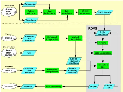
Meanwhile, ROPS has been implemented for various re-gions in the world ocean, and has been running automatically without any major interruptions since early 2015. The con-cept (Fig. 1) for all realisations is identical: every day, ROPS is initialised from a restart file of the previous day’s run, and it provides a 3-day forecast relative to the present. For each run, data sets for the definition of initial and boundary condi-tions plus observational data for assimilation are downloaded from the internet, in which the initial conditions are only re-quired for re-initialisation of ROPS in the case that it died the day before.

For this article, ROPS is slightly modified: it is run in hind-cast mode for a period of time in June 2014. All data for

model initialisation, boundary conditions, and a huge set of observational data for assimilation are available on the local computer system and a download from the internet is not re-quired. The objectives are to demonstrate the following:

– Good forecasts can be obtained from a prediction sys-tem using OA for assimilation (for the definition of “goodness”, see Murphy, 1993).

– A vast number of observational data can be managed by OA without data reduction by averaging, sub-sampling, or creating “super observations” (Lorenc, 1981; Moore et al., 2011b; Oke et al., 2015).

– ROPS is able to provide timely operational forecasts even on a commercially available personal computer or a laptop.

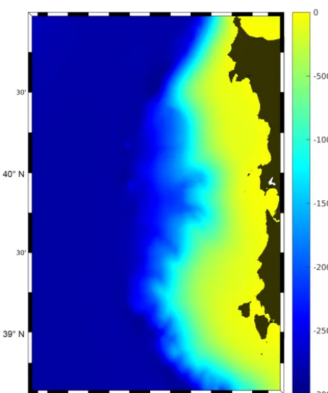
The area of the ROPS model domain (Fig. 2) is charac-terised by a 20–50 km wide continental shelf. The shelf ends at water depths between 150 and 200 m, followed by the con-tinental slope which features several canyons. The deep-sea area belongs to the northern Algerian Basin (also referred to as the Sardo-Balearic Basin) and exhibits water depths of up to 2800 m. According to Millot (1999), the mean surface cir-culation is mainly related to the inflow of “new” Modified Atlantic Water (MAW) from the Strait of Gibraltar by means of anticyclonic eddies originating from the Algerian Current. Another branch of “old” MAW, which mixed with the un-derlying water masses on its large-scale cyclonic circulation through the Tyrrhenian, Ligurian, and Balearic seas, comes probably from the west via the Balearic Current (García et al., 1996). Just below the MAW, Winter Intermediate Water (WIW) follows the path of the MAW along its whole cy-clonic path. Levantine Intermediate Water (LIW) originates from the eastern Mediterranean and the direct path to the ROPS domain is via the Sardinia Channel and then north-ward around the southern tip of Sardinia. Below the LIW, Western Mediterranean Deep Water (WMDW) and Bottom Water (BW) are found.

Figure 1.The ROPS concept: web resources are depicted by clouds, blue parallelograms represent data sets on the local host, and processes are indicated by green rectangles. The processing of ROMS is accomplished within the grey box.T andSdenote temperature and salinity, respectively.

occurred also to the west of the 1000 m contour in a broad 30–50 km wide band but in addition, there was a narrow vein of near-coastal northward currents, the width of which rarely exceeded 10 km. Southward transport with a zonal extent of 20–40 km prevailed between the two northward-directed regimes. Both the meridional flow bands of MAW and LIW were connected by alternating 10–30 km wide zonal currents. The observed geostrophic flow pattern suggests a mean trans-port to the north with superimposed mesoscale perturbations of 10–40 km in diameter. This defines another demand to ROPS to reproduce the horizontal variability of these scales, i.e. to resolve the Rossby radius. Concerning the temporal scales, repeated ADCP (acoustic Doppler current profiler) sections indicated that noticeable changes of the flow field occurred within 4 days (see Fig. 14 in Knoll et al., 2017). However, this timescale was stipulated by the minimum in-terval between the repeated ADCP surveys; in reality, shorter scales are likely. Hence, an additional objective is to resolve at least day-to-day changes.

The modified version of ROPS is described in Sect. 2. Sec-tion 3 provides an overview of the observaSec-tional data used in the framework of this article. The results of various ROPS

runs are presented in Sect. 4 and discussed in Sect. 5. The conclusions are found in Sect. 6. All time specifications refer to the year 2014, and the time standard UTC (Coordinated Universal Time).

2 ROPS 2.1 ROMS

Figure 2.The ROPS domain; the colour code indicates the water depth (m) after smoothing.

mixing of momentum and tracers is accomplished by means of a Laplacian formulation, and the vertical mixing is param-eterised by the GLS (generic length-scale) scheme (Umlauf and Burchard, 2003) using the k–ωsetup based on the turbu-lent closure scheme of Wilcox (1988). The air–sea interac-tion boundary layer in ROMS is formulated by means of the bulk parameterisation of Fairall et al. (1996). The processing of ROMS is accomplished within the grey box depicted in Fig. 1, including nudging, data assimilation, and the proper integration.

2.2 The domain

While the processing of ROMS is recurring, the setup of the ROPS domain is a one-time task (Fig. 1). The domain is situ-ated to the west of Sardinia (Fig. 2). The west and east bound-aries are at 6◦30.50 and 8◦35.50E, while in the south and north the domain is limited by the 38◦36.40and 40◦59.60N latitude circles, respectively. In the east–west direction, the domain is separated into 120 grid cells, and in the south– north direction into 178 cells, which yields an average grid spacing of1x≈1y≈1500 m in the zonal and meridional direction, respectively.

Bathymetry data from the General Bathymetric Chart of the Oceans (GEBCO) with a spatial resolution of 1 arc min were provided by the British Oceanographic Data Centre (BODC) and mapped on the horizontal grid. Coastline data

from NOAA (National Oceanic and Atmospheric Adminis-tration) were overlaid on the bathymetry and required some manual editing of the land mask. In order to avoid crowding of thescoordinates in shallow water regions, the bathymetry was clipped at 20 m, which is the minimum allowed water depth. For the smoothing of the bathymetry, a second-order Shapiro filter was applied. After smoothing, the so-calledrx0 parameter resulted as 0.31, which is about 50 % higher than the maximum value of 0.2 recommended by Haidvogel et al. (2000), butrx0is still less than 0.4 as suggested in the ROMS forum (https://www.myroms.org/forum).

In the vertical direction, the domain is separated into

K=70s layers, with position controlled by three parame-ters (θs, θb, hc) and two functions,Vtr, Vstr. Here,Vtr is the transformation equation,Vstrthe vertical stretching function, θsandθbare the surface and bottom control parameters, and hcis the critical depth controlling the stretching (for more de-tails, see https://www.myroms.org/wiki/). For all ROMS runs shown below,Vtr=2, Vstr=1,θs=5, θb=0.4, hc=50 m were selected, enabling high vertical resolution near the sur-face. This combination of functions and parameters yielded a grid-dependent parameterrx1=22.7, which is a measure for the pressure gradient error over steep topography. In fact, according to the ROMS discussion forum,rx1>14 is con-sidered as “insane” because the Haney (1991) condition is violated. However, various contributions in the forum report that even withrx114 no problems arose with the corre-sponding ROMS runs.

2.3 Initialisation and nudging

ob-servations. Moreover, precursor tests of ROMS using a grid size of 3000 km (nesting ratio∼3.1) revealed no significant differences compared to the actual version, except that small mesoscale features were not reproduced. This is in agreement with Pham et al. (2016), who demonstrated that the magni-tudes of errors were comparable, using nesting rations of 3 or 6, respectively.

After downscaling, all fields were interpolated vertically from the horizontal depth levels to thescoordinates. A spe-cial issue was the alignment of the land masks: if any wet grid cell in ROMS was covered by a dry grid cell of the par-ent, a smooth transition of all variables was created by taking the average of the surrounding parent cells. However, as this may lead to a violation of continuity by non-zero horizontal velocities normal to the land mask, all horizontal velocities next to the ROMS land mask were set to zero.

Later, during the course of the ROMS integration, there is the option to nudge the 3-D temperature and salinity fields once a day towards the parent. This guarantees that ROMS will not develop a solution in the interior of the domain which deviates significantly from the solution provided by the par-ent. This option is only useful if there are no data for assimi-lation, but in all model runs described in this article, nudging is turned off because a rich data set from observations was available (see below).

2.4 Lateral boundary conditions

The ROMS code includes various methods for the treatment of open boundaries. After extensive sensitivity studies, it was found that the following algorithms served best for the posed problem: for the sea surface elevation, the Chapman condi-tion was selected (Chapman, 1985), and for all other quanti-ties (i.e. barotropic and baroclinic momentum, turbulent ki-netic energy, eddy diffusivity), the mixed radiation-nudging conditions after Marchesiello et al. (2001) were applied.

The lateral time-dependent boundary conditions were pro-vided as well by MERCATOR by means of one-way nesting. However, the information was not instantaneously superim-posed to the ROMS solution but an additional nudging was applied to all prognostic variables which allowed these fields to adjust slowly to the parent values at the boundaries within ane-folding timescale of 2 days.

2.5 Surface boundary conditions

At the sea surface, boundary conditions for the air–sea ex-change of fresh water, momentum, and heat were eval-uated from the output of the COSMO-ME weather pre-diction model which was made available by the Italian Weather Service CNMCA (Centro Nazionale di Meteorolo-gia e ClimatoloMeteorolo-gia Aeronautica). COSMO-ME covers the en-tire Mediterranean Sea with a horizontal resolution of 7 km and provides 72 h forecasts of the wind field at 10 m height, air temperature and relative humidity at 2 m, air pressure at

sea level, cloudiness, short wave radiation, and precipitation. The temporal resolution is 1 h.

2.6 Data assimilation

In the ROPS runs presented below, temperature and salinity data from shipborne CTD (conductivity–temperature–depth) probes and gliders were assimilated. During the integration of ROMS, OA is controlled by six parameters:

– W: this is the width of the time window (in hours) that determines which data are selected for assimilation.W

is centred around the instanttassim when the assimila-tion takes place; e.g. if tassim=00:00 UTC (midnight) andW=24 h, data between noon of the previous day and noon of the successive day are selected.

– C: the correlation length scale (in km). C is a two-element vector enabling a non-isotropic Gaussian cor-relation for the meridional and zonal directions, respec-tively.

– δTobs,δSobs: the observational errors of temperature and salinity.

– δTb, δSb: the background errors of temperature and salinity.

Provided that all temperature and salinity data are stored as vertical profiles in daily directories, the data assimilation en-gine is invoked each day at midnight and proceeds as follows: – The daily directories are searched for CTD profiles

which fit in the desired time windowW.

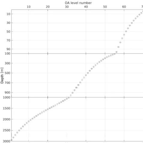
– The vertical levels are defined where the OA is per-formed; these levels are given by the depth of thes co-ordinates at the maximum depth of the domain (Fig. 3). – The vertical profiles are interpolated vertically on the

OA vertical levels.

– As the correlation length scale C is given in metric units, the ROMS spherical horizontal coordinates and the coordinates of the observations are converted to the metric Gauss–Krüger system.

– For each OA vertical level, the model prediction at the positions of the observations serves as background field for any tracer variable9(here: temperatureT and salin-ityS), and is subtracted from the observed data. – OA maps the anomalies at each level on the ROMS

hor-izontal grid and computes the normalised mapping error

9at the same time.

Figure 3.Depth of the vertical levels where the objective analysis (OA) is executed.

– The resulting tracer fields are melded with the actual ROMS fields, using 9 for weighting. As 0≤9≤1,

the melding for any tracer is accomplished by the algo-rithm

9corr=99ROMS+(1−9)9obs, (1) where 9ROMS is the original tracer field predicted by ROMS, 9obs are the gridded observations, and 9corr is the final corrected field resulting from the melding. Hence, if9is big (e.g.9=1 in the extreme case), no

correction is applied and the ROMS solution remains unchanged. At the other extreme (9=0 if the

obser-vations are 100 % trustworthy), the ROMS solution is rejected and substituted by the observations.

2.7 Integration and output

All ROPS runs presented below were initialised on 1 June at 00:00 UTC and integrated forward for 24 days until 25 June 00:00 UTC. From a precursor run, it was verified that the spin-up period was about 7 days. Hence, as the majority of observations are assimilated after 8 June, a statistical equilib-rium is almost achieved at that time. To satisfy the horizontal and the vertical CFL (Courant–Friedrichs–Lewy) criterion, a baroclinic time step of 108 s (800 steps per day) was cho-sen, and the number of barotropic time steps between each baroclinic time step was 40. Harmonic mixing along isopyc-nals with an eddy diffusivity coefficient of 5 m2s−1was used for the horizontal diffusion ofT andS, and a viscosity

co-efficient of 10 m2s−1 was selected for the diffusion of mo-mentum. In the vertical direction, a diffusivity coefficient of 2×10−5m2s−1_{was used and the eddy viscosity coefficient} was 10−5m2s−1. All diffusion coefficients were optimised in Onken (2017). Further on, a quadratic law using a coefficient of 0.003 was applied for the bottom friction, and the pressure gradient term was computed using the standard density Jaco-bian algorithm of Shchepetkin and Williams (2001, unpub-lished; see http://www.atmos.ucla.edu/~alex/ROMS/pgf1A. ps). The 3-D volume of all prognostic fields was written to an output file in 6 h intervals.

3 Observational data

Observational data were selected from the REP14-MED ex-periment which took place over the period 6–25 June; for a complete overview of all observations, see Onken et al. (2018). Some details are as follows:

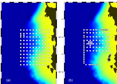
– 312 CTD casts taken by lowered CTD and underway CTD probes, of which there were 113 on Leg 1 (6–11 June), 173 on Leg 2 (12–20 June), and 26 at the start of Leg 3 on 23 June (for the casts on Legs 1 and 2 see Fig. 4). The positions of the casts taken during Leg 1 were arranged nominally on a 10 km×10 km grid ex-cept for two additional casts at 40◦150N (Fig. 4a). Dur-ing Leg 2, the samplDur-ing pattern of Leg 1 was partly repeated, but extra casts were taken at the boundaries of the observational grid. Further CTD profiles close to the Sardinian coast between about 39◦₁₅0_{and 39}◦₃₀0_N came from an acoustic experiment (Fig. 4b). The sched-uled vertical extent of all casts was 1000 dbar or bot-tom depth (whatever was shallower) but 10 casts espe-cially at the western boundary of the observational do-main reached greater depth to characterise the deep wa-ter masses.

– 5731 CTD profiles collected by 11 gliders (Fig. 5). All gliders were deployed on 8 and 9 June, and operated until their recovery on 23 June, except for the northern-most one, which died on 10 June. The nominal glider tracks were arranged halfway between the zonal CTD sections (Fig. 4), thus doubling the meridional resolu-tion of the observaresolu-tions. The scheduled depth of the gliders was limited by their pressure rating: six glid-ers were rated at 1000 dbar, one at 650 dbar, and four at 200 dbar.

– CTD data from ScanFish (EIVA, Skanderborg, Den-mark) tows between 21 June 12:03 UTC and 23 June 23:38 UTC (Fig. 6). The scheduled maximum depth of the ScanFish was around 190 m.

Figure 4.Positions of lowered CTD (circles) and underway CTD (triangles) casts collected during(a)Leg 1 (6–11 June) and(b)Leg 2 (12–20 June) of the REP14-MED experiment. The first casts were taken on 7 June. The colour code for the water depth is the same as in Fig. 2.

Fig. 7 are shown the number of CTD profiles which were available for assimilation.

4 Results

In the following are presented the results of four series of ROPS experiments. Series A explores the performance of the ROPS forecasts in terms of dependence on the correlation length scale, Series B explores the sensitivity to the back-ground errors, and Series C the impact of the size of the as-similation window. Finally, the dependence on the forecast range is assessed in Series D.

4.1 The verification method

The verification of the forecast accuracy is conducted by means of root-mean-square error (RMSE) analyses which acts as a metric for the difference between the observations and the forecasts of any tracer variable9. If there areN ob-servations andN corresponding forecasts, then the squared error of theith observation is

(19)2=9OBS(xi, yi, zi, ti)−9FC(xi, yi, zi, ti) 2

, (2)

wherex, y, zare the horizontal (eastward and northward) and vertical coordinates, respectively,tis time, and the subscripts

OBS and FC refer to the observations and the forecasts, re-spectively. The RMSE,19, of all observations is then

19=

v u u t 1

N N X

i=1

(9OBSi−9FCi)2. (3)

The forecast quality is determined by the skill score0, which is evaluated by means of the improvement of the forecast against a reference field (Murphy, 1988):

09=1−

19(FC,OBS)

19(REF,OBS), (4)

where 19(FC,OBS) is the RMSE between the forecast and the observations at the forecast time t=tFC, and 19(REF,OBS)is the RMSE between a reference field and the observations. Here, the values of T,S, and the poten-tial densityσ at the positions of the observations and at the instantt=tINI when the forecast was initialised, are serv-ing as reference (persistence assumption). Hence, a perfect forecast would yield 09=1 because the forecast agrees

exactly with the observations and 19(FC,OBS)=0. A successful or good forecast would mean19(FC,OBS) < 19(REF,OBS) and 0≤09≤1 because the forecast is

Figure 5.Surfacing positions of gliders, collected between 8 and 23 June. Each glider is marked by a different colour. The glider tracks are numbered G01–G10. G08 was occupied by two gliders. The colour code for the bathymetry is the same as in Fig. 2.

persistence”). By contrast, 09≤0 would be a criterion for

an unsuccessful or bad forecast because 19(FC,OBS) > 19(REF,OBS). In the following,09is applied both to

sin-gleslayers and to the mean:

09=

1

s2−s1+1 s2 X

s1

1− 19wgt(FC,OBS) 19wgt(REF,OBS)

, (5)

which is the average over all s layers from s layer no. s1 tos layer no.s2. The subscript wgt indicates weighting by the layer thickness in order to take account of the different masses of each layer.

In all ROPS runs presented below, the data from the Scan-Fish survey were utilised for verification. As the survey was completed within about 60 h, it was considered to be syn-optic and centred at t=tVER=22 June 18:00.19 and09 were evaluated at the same instant; hencetVER=tFCand the time dependence in Eq. (2) was removed. The synopticity assumption was somewhat risky because the expected scales of the temporal variability were less than 4 days (see Intro-duction). However, assuming non-synoptic conditions would have required us to interpolate the ROMS tracer output in 3-D space and time for each observation, or vice versa, to inter-polate each observation in the ROMS grid. Either of these ap-proaches would have been too expensive. Moreover, neither of them was necessary because the results shown below are

Figure 6.Tracks of the ScanFish tows (21–23 June) of the REP14-MED experiment.

consistent and conclusive. In order to make the ScanFish ob-servations suitable for a comparison with the ROMS model output, the trajectories were separated into 629 upward and downward profiles, and a mean time and a mean position were assigned to each profile. All temperature and salinity profiles were mapped with OA to constant depth levels on the ROMS horizontal grid, using a correlation scaleC=1.8 km. Thus, as the along-track distance between the individual pro-files was 500–700 m, three to four observations were con-tributing significantly to the mapping at each horizontal grid point. Finally, the analysed fields were interpolated from the horizontal OA levels on the ROMS vertical grid.

The observational errors for temperature and salinity,

Figure 7.Number of profiles available for assimilation during the period 7–23 June. Profiles from shipborne CTD probes, underway CTD, and gliders are included. The dates on the abscissae indicate the start of each day at 00:00 UTC.

Figure 8. Observed (a)temperature (◦C),(b) salinity, and(c)potential density (kg m−3) along the southernmost zonal ScanFish (SF) Sect. A09 (see Fig. 6). The positions of the ScanFish profiles are indicated by the magenta tick marks along the lower xaxis. Gridded (d)temperature,(e)salinity, and(f)potential density using objective analysis (OA). The tick marks indicate the OA grid. OnlyT andS

underwent OA while potential density was computed fromT,S, and depth.

19in Eqs. (3) and (4) was multiplied by(1−9). As9=0

at the exact position of the observation and 0< 9≤1

else-where,19 became significantly different from zero only in the immediate vicinity of the observation.

4.2 Series A: the impact of the correlation length scale

The natural correlation scale is the internal Rossby radius which in the western Mediterranean Sea lies between 3 and 13 km for the second and the first mode, respectively, de-pending on the season (Grilli and Pinardi, 1998; Robinson

between the glider tracks was also about 10 km, but the zonal resolution was O(100 m) in shallow water and O(1000 m) in deeper water. In this series, eight ROPS runs with differ-ent assumptions for the correlation length scaleCwere con-ducted.C was selected isotropic because a preliminary pro-cessing of data from shipborne ADCPs had revealed that the major part of the model domain was characterised by an eddy field with alternating currents; only along the west coast of Sardinia were predominantly meridional currents prevailing in a≈10 km wide stripe. The selected values forCwere 2.5, 5.0, 7.5, 10.0, 12.5, 15.0, 17.5, and 20 km, respectively.

In Series A, all CTD and glider data which were col-lected untiltINI=18 June 00:00 UTC were assimilated. The size of the assimilation window wasW=24 h. The obser-vational errors were set to fixed values δTobs=1.3◦C and δSobs=0.2 in all OA layers; these were the maximum val-ues of the respective standard deviations found in the upper thermocline. In precursor tests,δ9obswas set to the standard deviation of9 at the respective OA level (as was done for the OA of the ScanFish observations; see above), but here this strategy failed because in the deeper layers the standard deviation was approaching zero due to the horizontal homo-geneity of the water body, and the OA package generated unrealistic solutions which caused ROMS to die shortly af-ter the instant when data were assimilated. For similar rea-sons, δ9b was not derived from the standard deviation of the background field because the isotherms and isohalines in the deep ocean were almost horizontal which originated from the MERCATOR solution. Therefore, δ9b=δ9obsor r9=δ9b/δ9obs=1 was selected as a first guess. This was a rather conservative approach but it enabled the OA to find the optimum solution about halfway between the observa-tions and the background fields. After the last assimilation on 18 June, ROMS was integrated forward in a free mode – i.e. it was no longer constrained by observations. Finally, the model results were verified against the ScanFish obser-vations attFC=22 June 18:00 UTC. For an overview of the parameter settings and results, see Table 1.

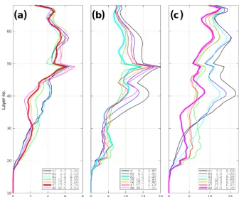
Figure 9 shows the vertical distributions of1T,1S, and

1σ for ROPS runs A1–A3 and A5–A8 (Run A4 is missing; it died on 14 June shortly after midnight, apparently because ROMS could not cope with the density field created by the assimilation). These quantities are evaluated in the ROMS vertical layers and plotted vs. the layer number, starting with layer 1 at the seabed. The graphs are empty for layers 1–9 and 69–70 next to the sea surface because the corresponding depth ranges were never reached by the ScanFish. In order to have an objective measure which correlation scale provided the best forecast,19 was averaged over all layers. The re-sulting layer thickness-weighted mean values1T,1S, and

1σ are written in the rightmost column of the legend of the graph and in Table 1 as well. Generally, 19 is decreasing from the surface to greater depth. However, rather low val-ues are found in layer 68, which covers the vertical range between about 7 m at the maximum depth of the domain

(see Fig. 3) and 0.6 m in the shallowest regions. This layer is characteristic for the mixed layer, the properties of which are controlled by the larger-scale uniform weather patterns. The maxima below in layer 49 are caused by the higher spa-tial variability in the thermocline as this layer ranges from about 10 to 220 m depth.1T lies between 2.74×10−3◦C in A7 and 3.11×10−3◦C in A2 but the variance among all runs is rather small. For1S, the minimum of 6.20×10−4is found in A3 and the maximum of 8.80×10−4in A1.1σ is minimum in A8 (5.59×10−4kg m−3) and the maximum of 8.68×10−4kg m−3is attained in A1. Hence, for1σ, there is a clear tendency that an increase in the OA correlation length scale appears to improve the accuracy of the forecast. Similar tendencies may be seen for1T and1S.

The vertical distributions of the skill scores09 and the corresponding layer weighted means are displayed in Fig. 10. Positive scores indicating a successful forecast of tempera-ture were obtained in all runs (except for A4, which died), and the maximum of0T =27.0 % was attained in A5. For

salinity, only the A3 and A5 forecasts beat persistence but with a rather low score of only 4.3 and 0.2 %, respectively.

0σ was positive for runs A1 and A3–A8, and the highest

score of 26.4 % was achieved in A5 forC=12.5 km. This is remarkably in line with Grilli and Pinardi (1998), who found the first-mode Rossby radius between about 11 and 13 km in the waters to the west of Sardinia.

Compared to the RMSE analysis above, the mean skill scores do not exhibit any correlation-scale-dependent trend. Instead, there are maxima of0T in A5,0S in A3, and0σ

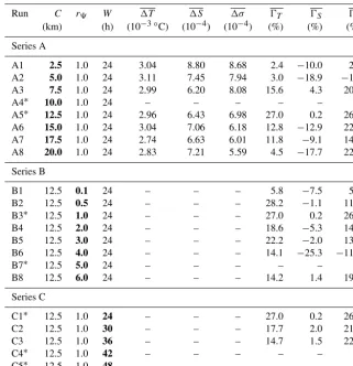
Table 1.Parameter settings and results of ROPS runs in Series A, B, and C. Bold numbers indicate those parameters which are varied within the respective series. The best run of each series is marked by an asterisk and serves as the control run for the successive series. Runs which died are marked by the∗symbol.

Run C r9 W 1T 1S 1σ 0T 0S 0σ

(km) (h) (10−3◦C) (10−4) (10−4) (%) (%) (%)

Series A

A1 2.5 1.0 24 3.04 8.80 8.68 2.4 −10.0 2.5 A2 5.0 1.0 24 3.11 7.45 7.94 3.0 −18.9 −1.0 A3 7.5 1.0 24 2.99 6.20 8.08 15.6 4.3 20.5 A4∗ 10.0 1.0 24 – – – – – – A5∗ 12.5 1.0 24 2.96 6.43 6.98 27.0 0.2 26.4 A6 15.0 1.0 24 3.04 7.06 6.18 12.8 −12.9 22.1 A7 17.5 1.0 24 2.74 6.63 6.01 11.8 −9.1 14.9 A8 20.0 1.0 24 2.83 7.21 5.59 4.5 −17.7 22.9

Series B

B1 12.5 0.1 24 – – – 5.8 −7.5 5.4 B2 12.5 0.5 24 – – – 28.2 −1.1 11.9 B3∗ 12.5 1.0 24 – – – 27.0 0.2 26.4 B4 12.5 2.0 24 – – – 18.6 −5.3 14.0 B5 12.5 3.0 24 – – – 22.2 −2.0 13.0 B6 12.5 4.0 24 – – – 14.1 −25.3 −11.2 B7∗ 12.5 5.0 24 – – – – – – B8 12.5 6.0 24 – – – 14.2 1.4 19.8

Series C

C1∗ 12.5 1.0 24 – – – 27.0 0.2 26.4 C2 12.5 1.0 30 – – – 17.7 2.0 21.7 C3 12.5 1.0 36 – – – 14.7 1.5 22.3 C4∗ 12.5 1.0 42 – – – – – – C5∗ 12.5 1.0 48 – – – – – –

4.3 Series B: the impact of background errors

In Series B, the dependency of 09 on δ9b was investi-gated while δ9obs was kept constant. Eight different con-figurations B1–B8 were tested using r9=δ9b/δ9obs∈ {.1, .5,1,2,3,4,5,6}. As r9 was continuously increasing

with increasing sequence number, the weighting of the back-ground field decreased at the same time and the objectively analysed temperature and salinity were forced closer to the observations. Note that B3 was the control run identical to A5.

As can be seen from Fig. 12, the mean forecast skill for temperature was positive for all runs and the maximum of

0T =28.2 % was attained in B2 using a ratior9=0.5. Thus, a background error of half the observational error produced the best forecast. For r9=0.1, 0T dropped suddenly to

5.8 % in B1 but increasingr9from 0.5 to 6.0 in B8 caused a

smooth decrease from the maximum in B2 to 14.2 % in B8. For salinity,0Swas mostly negative or close to zero, and the

best skill score of 1.4 % was obtained in B8 forr9=6.0.

De-spite the negative score for salinity,0σ was always positive

except for Run B6; the highest score of 26.4 % was recorded

in B3 usingr9=1. Therefore, B3 served as control run in

the subsequent Series C.

4.4 Series C: the impact of the assimilation window

In all previous runs, the data assimilation engine was in-voked each day at 00:00 UTC. As the size of the assim-ilation window was W=24 h, observational data between noon of the previous day and noon of the actual day were assimilated. This setting forW was the minimum because smaller values would lead to non-consideration of data. In this section, the impact of larger windowsW on the skill score is investigated in the five ROPS runs C1–C5, applying

Figure 9.The vertical distributions of(a)1T,(b)1S, and(c)1σ, for ROPS runs A1–A8. The first column in the legend boxes refers to the number of the ROPS run, the second column is the selected correlation scaleC(km), and the third column features the layer thickness-weighted mean19, where9stands for either tracerT,S, orσ. For better readability,1T was multiplied by 103, and1S,1σby 104. The bold graphs indicate the runs where19were minimal.

a model crash, but one has to consider that the gliders pro-vided up to more than 400 profiles every day (see Fig. 7), and an extension of W by just 6 h would mean that about 100 additional profiles, which were too decorrelated in time with the actual forecast, would contribute to the assimilation fields. The skill scores of the remaining runs C1–C3 are dis-played in Table 1. The best score for0σ was again reached

in the control Run C1; but also in C2 and C3, the scores were higher than 20 %. Worthy of mention are the positive but rather small scores for0Sin C2 and C3. In any case,

be-cause of the maximum scores for0tand0σ, C1 was selected as control run in the following Series D.

4.5 Series D: the impact of the forecast range

In this series, 12 ROPS runs D1–D12 with different forecast ranges were conducted and verified as before. In all runs, the parameter settings of C1 were utilised but the initialisa-tion time tINI, i.e. the time when the last data assimilation took place, was varied between 11 and 22 June. In D1, CTD data were assimilated until 11 June 00:00 UTC. Thereafter, ROMS was integrated forward in a free mode, i.e. it was no more constrained by observations. The forecast range τ

was the time span between the instant when the last assim-ilation took place and the verification time tFC=22 June

Table 2.Parameter settings and results of ROPS runs in Series D. Bold numbers indicate those parameters which are varied within this series.

Run t_INI τ 0T 0S 0σ 0σ(D0) (days) (%) (%) (%) (%)

D1 11 June 11.75 28.1 12.0 31.9 25.4

D2 12 June 10.75 32.9 11.1 29.7 24.8

D3 13 June 9.75 34.0 6.1 31.7 24.7

D4 14 June 8.75 23.5 0.7 24.4 15.5

D5 15 June 7.75 4.0 −5.0 11.3 10.2

D6 16 June 6.75 9.8 −16.4 12.6 12.9

D7 17 June 5.75 7.9 −4.2 18.2 1.0

D8 18 June 4.75 25.9 −4.3 25.5 1.3

D9 19 June 3.75 7.5 −3.9 10.0 −3.0

D10 20 June 2.75 −6.7 −6.1 4.1 4.8

D11 21 June 1.75 −17.5 −13.5 −22.4 −1.9

D12 22 June 0.75 5.8 −1.9 0.8 3.1

18:00 UTC, thus 11.75 days. In D2, the last data were as-similated on 12 June, in D3 on 13 June and so on. Hence, in runs D2–D12,tINIwas advanced by 24 h in each case un-til tINI=22 June 00:00 UTC in D12, and correspondingly the forecast range shrunk progressively in 1-day steps from

Figure 10.The vertical distributions of(a)0T,(b)0S, and(c)0σ, for ROPS runs A1–A8. The first column in the legend boxes refers to the

number of the ROPS run, the second column is the selected correlation scaleC(km), and the third column is the layer thickness-weighted mean09, where9stands for either tracerT,S, orσ. The bold graphs indicate the runs where19were maximal.

The skill scores of all runs in dependence ontINIandτ are summarised in Table 2, and in Fig. 13 are shown the graphs of0T,0S, and0σ. For D1 (tINI=11 June,τ=11.75 days), 0σ attained the absolute maximum of 31.9 % within this se-ries (Fig. 13c). Skill scores around 30 % were also reached in D2 and D3. In D4–D12 towards smaller forecast ranges, the score exhibited an overall decreasing trend but it remained positive except for D11 where0σ = −22.4 %. The

charac-teristics of the 0T curve closely resemble those of0σ. In

terms of qualitative arguments, the high scores are in D1– D3, and they decrease afterwards. Quantitatively, these are the scores around or even above 30 % in D1–D3, the moder-ate values around and below 10 % in D5 and D6, the scores above 25 % at the relative maximum in D8, the minima in D11, and the recovery to positive values in D12. The 0S

curve is correlated with the graphs of0σ and0T, concerning the overall decreasing trend and the locations of the relative minima and maxima. However, the skill scores for salinity are always lower than those for density and temperature in D1–D9 and D12, frequently even being negative. The high-est values above 10 % are attained in D1 and D2 – a rather modest score compared to the≈30 % scores ofT andσ at the same time.

In order to assess the impact of the data assimilation as a whole, another ROPS run was conducted – referred to as D0. This run was identical to all other runs of Series D but no

data were assimilated at any time. For D0, the skill scores were computed in the same way as for D1–D12 for each initialisation time day between 11 and 22 June, and in ad-dition for “virtual” initialisations on 1–10 June. The corre-sponding curves (the thin lines) are overlain to the graphs of

09 in Fig. 13a, b, c. The skill scores of D0 are positive for

the majority of the initialisation timestINI. Negative values for0T are only obtained fortINI∈ {1,2,3}June, for0S and tINI∈ {15,17,18,19,21}June, and for0σandtINI∈ {19,21} June. Thus, although no data were assimilated in D0, the forecasts beat persistence in most cases for forecast ranges of at least 3 weeks. Other particular features of the D0 fore-casts are the maximum skill score fortINI=8 June and the decreasing trend thereafter. Except for D6 (tINI=16 June) and 20 June ≤tINI≤22 June, the skill scores 0σ of D0 are always lower than the corresponding scores of D1–D12. Hence, the assimilation of observational data has definitely improved the forecast quality for potential density. A simi-lar proposition is valid for0T but not for0S. Here, except

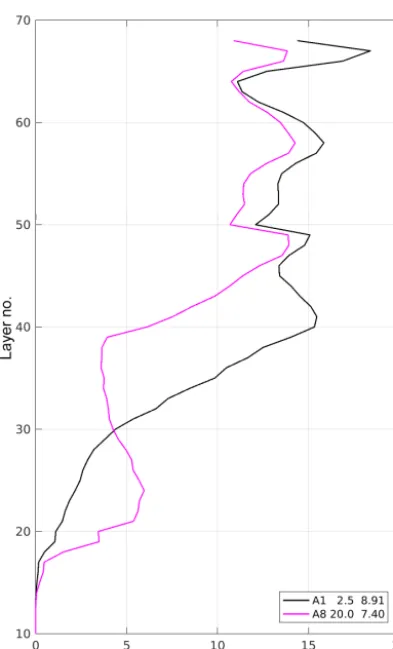
Figure 11.The vertical distributions of1σ (REF, OBS)for ROPS runs A1 and A8 att=tINI=18 June 00:00 UTC. The first column in the legend boxes refers to the number of the ROPS run, the sec-ond column is the selected correlation scaleC (km), and the third column is the layer thickness-weighted mean1σ. For better read-ability,1σwas multiplied by 104.

5 Discussion

The first objective of this article was to demonstrate that ROPS produces good forecasts. Murphy (1993) defines three types of “goodness”: consistency, quality, and value. Con-cerning the latter, it is rather difficult to rate the value for the “end users” because REP14-MED was planned solely for scientific purposes – see the objectives defined in Onken et al. (2018). Amongst others, a special aim was the compari-son of different methods for data assimilation. This article is the third in a series of five, of which Oddo et al. (2016) and Onken (2017) have been published. Two further articles us-ing the same observational data are in preparation, applyus-ing the ensemble Kalman filter and 4D-Var assimilation meth-ods. Hence, the value of the ROPS forecasts may be best judged when all papers have been published. The consistency of the ROPS forecasts has been assessed by comparison with the observations described by Knoll et al. (2017), using the output of ROPS run C1 on 20 June. In detail, the

large-scale horizontal distributions of T and S at 50 and 400 m depth (these are the depths of the MAW and LIW cores, respectively) resembled the observed patterns, but the con-tours were shifted against each other by several miles. This was plausible because the observed fields were averaged over the observational period 8–18 June while the forecast was a snapshot. The same applied to the predicted currents which were checked against the observed geostrophic transports. It was also verified that the data assimilation did not create any unrealistic water masses in those regions where nearby ob-servations were available. In order to assess the impact of the large nesting ratio, the vertical velocity along the lateral boundaries was frequently checked for strange patterns, but no abnormal behaviour was detected at any time. This was not surprising, because to minimise false advection effects, the distance between the open boundaries and the observa-tions was 30 miles in the west and 45 miles in the south and the north (see Figs. 4, 5).

With respect to the forecast quality, a major result found above was that the mean skill scores 0T, 0S, and 0σ

de-creased concurrently with a decreasing forecast rangeτ. As this feature was observed both for the assimilation runs D1– D12 and for the free run D0, it can be excluded that it was somehow caused by the assimilation of observational data. Therefore, the components of the equation which deter-mine the skill score were investigated. In particular, a closer look was taken at19wgt(FC, OBS)and19wgt(REF, OBS) in Eq. (5). However, as these expressions represent the weighted RMSE of each individualslayer, it is not possible to relate them to the mean skill score09. Therefore, for the purpose of discussion, the mean skill score was re-defined as

0₉∗ =1− 19wgt(FC,OBS) 19wgt(REF,OBS)

. (6)

Here,0∗₉is the mean skill score computed from the mean layer RMSEs while09 as defined in Eq. (5) is the mean

score computed from the individual layer RMSEs. In Fig. 14 are shown1σwgt(FC,OBS),1σwgt(REF,OBS), and0∗σ for

D1–D12 and for D0, in dependence on the forecast rangeτ

(bottom axis) and simultaneously on the initialisation time

tINI(top axis). First of all,0∗σ and0σ in D1–D12 (compare

Figs. 14b, 13c) are almost identical, which legitimatises the re-definition in Eq. (6). By contrast, the shape of the corre-sponding graphs for the no-assimilation run D0 differ from each other: the0∗

σ curve is smoother than that of 0σ, but

the increasing trend for 1 June< tINI<8 June and the de-creasing trend thereafter are reproduced, which is important for this discussion. According to Fig. 14a,1σwgt(FC,OBS) (thin red line) is constant for all initialisation times tINI. This is trivial because the RMSE between the forecasted fields and the observations on 22 June never changes, re-gardless of the virtual initialisation time. This facilitates the discussion because the skill score depends now solely on

Figure 12.The vertical distributions of(a)0T,(b)0S, and(c)0σ, for ROPS runs B1–B8. The first column in the legend boxes refers to

the number of the ROPS run, the second column is the selected ratioδ9b/δ9obs(for9∈T , S), and the third column is the layer thickness-weighted mean09, where9stands for either tracerT,S, orσ. The bold graphs indicate the runs where19were maximal.

of the latter is identical to the shape of the0∗

σ curve which

means that for all initialisation times tINI> 8 June, the ROMS initial fields are progressively approaching the verifi-cation fields with increasingtINI. Apparently, some unknown process or combination of different processes is already driv-ing the model towards the future observations without data assimilation. Potential candidates could be the downscaling of the MERCATOR fields on 1 June (see above, Sect. 2.3) enabling a more realistic circulation pattern, the MERCA-TOR forcing at the lateral boundaries, or the daily updated COSMO-ME forecasts which would not be available in real operational conditions. The opposite is the case for tINI< 8 June: here, the ROMS initial fields deviate progressively from the verification fields with increasing tINI. Probably, ROMS needs a certain spin-up time to equilibrate all fields, which would be about 8 days in the present situation.

For the assimilation runs D1–D12, 1σwgt(FC,OBS) (Fig. 14a, bold red line with dots) is decreasing continu-ously with increasingtINI. Hence, the later ROMS switches to the free mode without data assimilation, the closer is the forecast to the observations. This is not trivial because each assimilation cycle could create “assimilation shocks” and mess up the model dynamics (Evensen, 2003; Counil-lon et al., 2016). Probably, this happened in D1–D5, where

1σwgt(FC,OBS) is at about the same level as the corre-sponding quantity in D0, but in D6–D12 (16 June≤tINI≤

22 June), 1σwgt(FC,OBS) is below the horizontal line, which indicates that the predicted density pattern is closer to the observations than in the no-assimilation run. This does not necessarily mean that the skill score is higher, because0∗ σ

depends on the ratio 1σwgt(FC,OBS)/1σwgt(REF,OBS) according to Eq. (6). As shown by the bold blue line with dots, the denominator is mostly greater than the numerator (except for D11), and also its overall slope is larger. Con-sequently, the ratio is mostly<1, leading to a positive skill score. Moreover, in D1–D4 and D7–D8, the ratio is small and correspondingly, the skill score is large. By contrast, in D5, D6, D9, D10, and D12 the ratio is close to 1 and the skill score is approaching zero. This effect also controls the over-all negative trend of the skill score because the numerator and the denominator are approaching each other with decreasing forecast rangeτ. In other words, if the forecast range is small, then the reference fields are already very close to the verifica-tion fields, and no significant improvement can be achieved by further forward integration of the numerical model.

In all runs shown above, except for D10 and D11 (see Ta-bles 1 and 2),0T was greater than0S, frequently even much greater. It can be excluded that this was due to an error in the OA or in the melding procedure (Eq. 1), as the same sub-routines were used for T and S. Additional evidence was found from D0: Fig. 13a, b clearly show that0S was always

Figure 13.The skill scores(a)0T,(b)0S, and(c)0σ vs. the forecast rangeτfor ROPS runs D0 and D1–D12. The June dates on the top

abscissae indicate the start of each day at 00:00 UTC; the dates are identical to the assimilation timetINI. Note that the time axis at the top is offset by 6 h with respect to the time axis at the bottom in order to synchronisetINIandτ.

OA or Eq. (1) was never applied in D0, neither could be the cause for this weird behaviour. Likewise, errors during the processing of the data for assimilation can be precluded. An-other possible source of error could be the computation of the forecast skills. However, the coding of Eqs. (2)–(5) was checked several times and no error was detected. Hence, it is concluded that some physical process is not properly param-eterised in ROMS, which induces the different skill scores of

T andS. A possible process is double diffusion which effec-tuates higher vertical diffusivities for salinity than for tem-perature (Schmitt, 1981). As shown by Zhang et al. (1998), the consideration of double-diffusive mixing in a general cir-culation model can have a significant impact on the hori-zontal transport of heat and salt, even if a conservative ap-proach is applied to the parameterisation. The stratification in the Mediterranean Sea is especially favourable for dou-ble diffusion because of the high-salinity core of LIW be-low the main thermocline (Millot, 1999). Onken and Bram-billa (2003) have shown that in the Algerian Basin and be-low about 300 m depth, the vertical diffusivity of salt may be

up to twice as high as the diffusivity of heat. This leads to an enhanced diffusion of buoyancy and similarly may affect the entire circulation pattern and the different skill scores for temperature and salinity.

MERCA-Figure 14. (a)1σwgt(FC, OBS),1σwgt(REF, OBS)and(b)0∗₉(see Eq. 6) vs. the forecast rangeτfor ROPS runs D0 and D1–D12. The June dates on the top abscissae indicate the start of each day at 00:00 UTC; the dates are identical to the assimilation timetINI. Note that the time axis at the top is offset by 6 h with respect to the time axis at the bottom in order to synchronisetINIandτ.

TOR global model against persistence. They demonstrated that for most regions the skill score was positive, except for the North Atlantic, the Mediterranean Sea, and Antarctica. Also in the framework of GODAE, Ryan et al. (2015) ver-ified six different forecasting systems against climatology and persistence. Their main results were that the climatol-ogy skill score of all systems was positive for all tested pa-rameters, while the persistence skill score (PSS) was close to zero or even negative for short forecast ranges, both for temperature and salinity. Afterwards, however, the PSS in-creased with longer forecast ranges of up to 5 days. More-over, the PSS of salinity was mostly lower than the PSS of temperature. Forecast skill assessments of regional mod-els have been conducted by various authors. Tonani et al. (2009) evaluated the forecast skill score of the Mediterranean Forecasting System (MFS; Pinardi (2003), horizontal resolu-tion ≈7 km) by means of comparisons with observational data from moorings, ARGO floats, and XBT (expendable bathythermograph) casts at three different vertical levels. It has been demonstrated that the skill scores of temperature and salinity increased with increasing forecast range, reach-ing a maximum of about 45 % for temperature around the sixth day of the forecast. This is about 30 % higher than the maximum skill score 0T determined above (see Sect. 4.5)

which was 34 % fortINI=13 June, corresponding to a fore-cast range of about 10 days. For the very short forefore-cast range of 2 days, the skill scores were negative, and right at the sur-face and in the upper thermocline, the skill score for salinity was mostly lower than for temperature. A generally lower

skill score for salinity, which is in agreement with the results of this article, was also found by Chiggiato and Oddo (2008) for two higher-resolution operational models of the Adriatic Sea. Tonani et al. (2009) also evaluated the components of the skill score. They demonstrated that 19(FC,OBS)and

19(REF,OBS)both for9≡T and9≡Swere approach-ing each other with increasapproach-ing forecast range; this is compa-rable to the findings of Fig. 14. On the whole, the sometimes surprising results of this article are in line with other publi-cations.

June; hence, 377 profiles were assimilated every day at mid-night on average. It would be worth exploring whether this potential oversampling leads to an improvement or even a deterioration of the forecast quality, compared to ROPS runs where fewer data would be assimilated, although this would first require the development of a meaningful methodology for data reduction. Different approaches for the reduction of observational data could be utilised to address a number of interesting questions:

– Are deep CTD casts needed to improve the forecast skill scores? Several deep casts extending to more than 2500 m depth were taken at the western boundary of the observational domain to assess the hydrography of the deep water masses.

– What is the impact of “deep” gliders on the skill score? During REP14-MED, four gliders had a pressure rating of 200 dbar, one was rated to 650 dbar, and six gliders took samples down to 1000 dbar. The impact of the deep gliders could easily be assessed if their profiles were clipped at 200 m.

– What is the cost / benefit ratio of adding more gliders? Eleven gliders were operating on 10 zonal tracks (see Fig. 5). Although the northernmost one died early, there were still nine tracks G02–G10 occupied continuously for more than 2 weeks. In the first run of a cost–benefit analysis, only the data of the glider on the central track G06 would be assimilated, in the second run data from tracks G02 and G10 would be added, the third run would assimilate data from tracks G02, G04, G06, G08, and G10, and in the final run, data from all tracks would be used. Thus, the meridional resolution would be doubled during consecutive runs, and the skill score versus the resolution could be assessed.

Answering these questions is beyond the scope of this paper, but might be addressed in a follow-up paper.

Finally, it was demonstrated that ROPS is able to provide timely forecasts on a commercially available personal com-puter. All ROPS runs were conducted on a DELL Precision Tower 7910 using four processors. The CPU time of D12, which performed the maximum of 16 assimilation cycles, was 4.8 h, while it was only 2.7 h for D0 without any assimi-lation. Hence, as ROPS was integrated over 24 days, the CPU time for solving the primitive equations was just 6.8 min per day. In the case that on average 377 CTD profiles were assim-ilated, the CPU time nearly triplicated to 18 min. This rather modest increase was effectuated by the pre-selection of ob-servational data in daily directories which considered only those data for assimilation which fitted in the time window

W. The triplicating of CPU time is still a reasonable figure compared to operational models employing 4D-VAR where the CPU time may increase by at least 1 order of magnitude.

6 Conclusions

The relocatable ocean prediction system (ROPS) was em-ployed in hindcast mode on a huge data set which was col-lected in June 2014. Using objective analysis (OA), the ob-servational data were assimilated, and the ROPS forecasts were verified against independent data.

The OA is controlled by four parameters:C, the correla-tion length scale;r9, the ratio of background and

observa-tional errors for temperature and salinity, respectively; and

W, the width of the time window where data are assimilated. Sensitivity tests to variations of these parameters were con-ducted by means of various ROPS runs encompassing the pe-riod 1–24 June. Observational data were assimilated for the period 7–18 June, and the forecasts were verified against the verification data set on 22 June. The highest skill scores were obtained forC=12.5 km,r9=1, andW=24 h.

Additional runs revealed a decreasing tendency of the skill score with decreasing forecast range, where the forecast range was the time span between the verification time and the instant when the last assimilation took place. The same tendency was exhibited by a control run without assimila-tion which excludes the OA from being responsible for this behaviour. A thorough analysis of the terms in the equation, which determines the skill score, revealed that persistence is approached steadily for continuously decreasing forecast ranges, and the late assimilation of observational data can no longer effectuate a significant improvement of the forecast skill. For extremely small forecast ranges, the skill score even became negative, because the assimilation disequilibrated the balance of forces in the dynamical model.

In all ROPS runs, including the run without assimilation, the skill score for temperature was mostly higher than the corresponding score for salinity. This is in agreement with other research papers, and it is speculated that this mismatch is due to double-diffusive processes which were not ade-quately parameterised.

ROPS is able to provide timely forecasts even on commer-cially available personal computers.

Code availability. All work related to this article was done on a Linux workstation under Kubuntu 16.04. ROMS/TOMS version 3.6 was used for the model runs, the pre- and postprocessing was done with MATLAB R2016b, and the article was written in LA_{TEX. The} model code and all scripts are available from the author on request.

Competing interests. The author declares that they have no conflict of interest.

Special issue statement. This article is part of the special issue “REP14-MED: A Glider Fleet Experiment in a Limited Marine Area”. It is not associated with a conference.

Acknowledgements. The author would like to thank the masters and crews of NRVAllianceand RVPlanetfor their professionalism during the conduction of the experiments at sea. The data from COSMO-ME were provided by the Italian weather service Centro Nazionale di Meteorologia e Climatologia Aeronautica (CNMCA) and the MERCATOR data sets were downloaded from the Coper-nicus Marine Environment Service (CMEMS). Bathymetry data from the General Bathymetric Chart of the Oceans (GEBCO) originated from the British Oceanographic Data Centre (BODC), and coastline data were obtained from the National Oceanic and Atmospheric Administration (NOAA). The author is grateful to the two anonymous reviewers who helped to improve the article. REP14-MED was sponsored by HQ Supreme Allied Command Transformation (Norfolk, VA, USA).

The article processing charges for this open-access publication were covered by a Research

Centre of the Helmholtz Association.

Edited by: Giovanni Quattrocchi Reviewed by: two anonymous referees

References

Bell, M. J., Lefèbvre, M., Le Traon, P.-Y., Smith, N., and Wilmer-Becker, K.: GODAE: The Global Ocean Data Assimilation Experiment, Oceanography, 22, 14–21, https://doi.org/10.5670/oceanog.2009.62, 2009.

Bretherton, F. P., Davies, R. E., and Fandry, C. B.: Technique for Objective Analysis and design of oceanographic experiments ap-plied to Mode-73, Deep-Sea Res., 23, 559–582, 1976.

Capet, X., McWilliams, J. C., Molemaker, M. J., and Shchep-etkin, A. F.: Mesoscale to submesoscale transition in the California Current system, Part I: flow structure, eddy flux, and observational tests, J. Phys. Oceanogr., 38, 29–43, https://doi.org/10.1175/2007JPO3671.1, 2008.

Centre for Maritime Research and Experimentation: REP14 data, available at: http://geos3.cmre.nato.int/REP14 (last access: 10 March 2017), La Spezia, Italy, 2014.

Chapman, D. C.: Numerical treatment of cross-shelf open bound-aries in a barotropic coastal ocean model, J. Phys. Oceanogr., 15, 1060–1075, 1985.

Chiggiato, J. and Oddo, P.: Operational ocean models in the Adriatic Sea: a skill assessment, Ocean Sci., 4, 61–71, https://doi.org/10.5194/os-4-61-2008, 2008.

Counillon, F., Keenlyside, N., Bethke, I., Wang, Y., Billeau, S., Shen, M. L., and Bentsen, M: Flow-dependent assimilation of sea surface temperature in isopcnal coordinates with the

Norwegian Climate Prediction model, Tellus A, 68, 32437, https://doi.org/10.3402/tellusa.v68.32437, 2016.

De Dominicis, M., Falchetti, S., Trotta, F., Pinardi, N., Giacomelli, L., Napolitano, E., Fazioli, L., Sorgente, R., Haley Jr., P. J., Ler-musiaux, P. F. J., Martins, F., and Cocco, M.: A relocatable ocean model in support of environmental emergencies, Ocean Dynam., 64, 667–688, https://doi.org/10.1007/s10236-014-0705-x, 2013. Dombrowsky, E.: Overview Global Operational Oceanogra-phy Systems, Chapter 16, in: Operational OceanograOceanogra-phy in the 21st Century, edited by: Schiller, A., and Brassing-ton, G. B., Springer Science+Business Media B.V., 397–411, https://doi.org/10.1007/978-94-007-0332-2_16, 2011.

Dombrowsky E., Bertino, L., Brassington, G. B., Chassignet, E. P., Davidson, F., Hurlburt, H. E., Kamachi, M., Lee, T., Martin, M. J., Meu, S., and Tonani, M.: GODAE Systems in Operation, Oceanogr., 22, 83–95, 2009.

Drévillon, M., Bourdallé-Badie, R., Derval, C., Lellouche, J. M., Rémy, E., Tranchant, B., Benkiran, M., Greiner, E., Guinehut, S., Verbrugge, N., Garric, G., Testut, C. E., Laborie, M., Nouel, L., Bahurel, P., Bricaud, C., Cros-nier, L., Dombrowsky, E., Durand, E., Ferry, N., Hernan-dez, F., Le Galloudec, O., Messal, F., and Parent, L.: The GODAE/Mercator-Ocean global ocean forecasting system: re-sults, applications and prospects, J. Oper. Oceanogr., 1, 51–57, https://doi.org/10.1080/1755876X.2008.11020095, 2008. Edwards, C. A., Moore, A. M., Hoteit, I., and Cornuelle, B. D.:

Re-gional Ocean Data Assimilation, Annu. Rev. Mar. Sci., 7, 21–42, https://doi.org/10.1146/annurev-marine-010814-015821, 2015. Evensen, G.: The Ensemble Kalman Filter: theoretical

formula-tion and practical implementaformula-tion, Ocean Dynam., 53, 343–367, https://doi.org/10.1007/s10236-003-0036-9, 2003

Evensen, G.: The Ensemble Kalman Filter: theoretical formula-tion and practical implementaformula-tion, Ocean Dynam., 53, 343–367, https://doi.org/10.1007/s10236-003-0036-9, 2003.

Fairall, C. W., Bradley, E. F., Rogers, D. B., Edson, J. B., and Young, G. S.: Bulk parameterization of air-sea fluxes for Tropical Ocean-Global Atmosphere Coupled-Ocean Atmo-sphere Response Experiment, J. Geophys. Res., 101, 3747–3764, https://doi.org/10.1029/95JC03205, 1996.

García-Ladona, E., Castellón, A., Font, J., and Tintoré, J.: The Balearic current and volume transports in the Balearic Basin, Ocean. Ac., 19, 489–497, 1996.

Grilli, F., and Pinardi, N.: The computation of Rossby radii of de-formation for the Mediterranean Sea, MTP news, 6, 4, 1998. Gula, J., Molemaker, M. J., and McWilliams, J. C.:

Subme-soscale dynamics of a Gulf Stream frontal eddy in the South Atlantic Bight, J. Phys. Oceanogr., 46, 305–325, https://doi.org/10.1175/JPO-D-14-0258.1, 2016.

Haidvogel, D. B., Arango, H. G., Hedstrøm, K., Beckmann, A., Malanotte-Rizzoli, P., and Shchepetkin, A. F.: Model evaluation experiments in the North Atlantic Basin: simulations in nonlinear terrain-following coordinates, Dynam. Atmos. Ocean., 32, 239– 281, 2000.

Haney, R. L.: On the pressure gradient force over steep topography in sigma coordinate models, J. Phys. Oceanogr., 21, 610–619, 1991.

and Circulation West of Sardinia in June 2014, Ocean Sci. Dis-cuss., https://doi.org/10.5194/os-2017-45, in review, 2017. Lellouche, J.-M., Le Galloudec, O., Drévillon, M., Régnier, C.,

Greiner, E., Garric, G., Ferry, N., Desportes, C., Testut, C.-E., Bricaud, C., Bourdallé-Badie, R., Tranchant, B., Benkiran, M., Drillet, Y., Daudin, A., and De Nicola, C.: Evaluation of global monitoring and forecasting systems at Mercator Océan, Ocean Sci., 9, 57–81, https://doi.org/10.5194/os-9-57-2013, 2013. Lorenc, A. C.: A global three-dimensional multivariate statistical

interpolation scheme, Mon. Weather Rev., 109, 701–721, 1981. Marchesiello, P., McWilliams, J. C., and Shchepetkin, A. F.: Open

boundary conditions for long-term integration of regional ocean models, Ocean Model., 3, 1–20, 2001.

Martin, P. J.: Description of the Navy Coastal Ocean Model Version 1.0, NRL/FR/7322-00-9962, Nav. Res. Labor., 42 pp., 2000. McWilliams, J. C.: Submesoscale currents in the ocean, P. Roy.

Soc. A, 472, 20160117, https://doi.org/10.1098/rspa.2016.0117, 2016.

Millot, C.: Circulation in the Western Mediterranean Sea, J. Mar. Syst., 20, 424–442, 1999.

Moore, A.M., Arango, H. G., Broquet, G., Powell, B. S., Weaver, A. T., and Zaval-Gray, J.: The Regional Ocean Modeling Sys-tem (ROMS) 4-dimensional variational data assimilation sys-tems, Part I: system overview and formulation, Prog. Oceanogr., 91, 34–49, 2011a.

Moore, A.M., Arango, H. G., Broquet, G., Edwards, C., Veneziani, M., Powell, B., Foley, D., Doyle, J. D., Costa, D., and Robin-son, P.: The Regional Ocean Modeling System (ROMS) 4-dimensional variational data assimilation systems, Part II: Per-formance and application to the California Current System, Prog. Oceanogr., 91, 50–73, 2011b.

Murphy, A. H.: Skill scores based on the mean square error and their relationships to the correlation coefficient, Mon. Weather Rev., 116, 2417–2424, 1988.

Murphy, A. H.: What is a good forecast? An Essay on the nature of goodness in weather forecasting, Weather Forecast., 8, 281–293, 1993.

Oddo, P., Storto, A., Dobricic, S., Russo, A., Lewis, C., Onken, R., and Coelho, E.: A hybrid variational-ensemble data assimilation scheme with systematic error correction for limited-area ocean models, Ocean Sci., 12, 1137–1153, https://doi.org/10.5194/os-12-1137-2016, 2016.

Oke, P. R., Larnicol, G., Jones, E. M., Kourafalou, V., Sperrevik, A. K., Carse, F., Tanajura, C. A. S., Mourre, B., Tonani, M., Brassington, G. B., Le Henaff, M., Halliwell Jr., G., R., Atlas, R., Moore, A. M., Edwards, C. A., Martin, M. J., Sellar, A. A., Alvarez, A., De Mey, P., and Iskandarani, M.: Assessing the im-pact of observations on ocean forecasts and reanalyses: Part 2, Regional applications, J. Oper. Oceanogr., 8, s63–s79, 2015. Onken, R.: Validation of an ocean shelf model for the prediction

of mixed-layer properties in the Mediterranean Sea west of Sar-dinia, Ocean Sci., 13, 235–257, https://doi.org/10.5194/os-13-235-2017, 2017.

Onken, R., Ampolo-Rella, M., Baldasserini, G., Borrione, I., Cec-chi, D., Coelho, E., Falchetti, S., Fiekas, H.-V., Funk, A., Jiang, Y.-M., Knoll, M., Lewis, C., Mourre, B., Nielsen, P., Russo, A., and Stoner, R.: REP14-MED Cruise Report. CMRE Cruise Report Series, CMRE-CR-2014-06-REP14-MED, CMRE, La Spezia, 76 pp., 2014.

Onken, R. and Brambilla, E.: Double diffusion in the Mediterranean Sea: observation and parameterization of salt finger convection, J. Geophys. Res., 108, 8124, https://doi.org/10.1029/2002JC001349, 2003.

Onken, R., Fiekas, H.-V., Beguery, L., Borrione, I., Funk, A., Hem-ming, M., Heywood, K. J., Kaiser, J., Knoll, M., Poulain, P.-M., Queste, B., Russo, A., Shitashima, K., Siderius, M., and Thorp Küsel, E.: High-resolution observations in the western Mediter-ranean Sea: the REP14-MED experiment, Ocean Science, in preparation, 2018.

Pham, S., Hwang, J. H., and Ku, H.: Optimizing dy-namic downscaling in one-way nesting using a re-gional ocean model, Ocean Model. 106, 104–120, https://doi.org/10.1016/j.ocemod.2016.09.009, 2016.

Pinardi, N., Allen, I., Demirov, E., De Mey, P., Korres, G., Las-caratos, A., Le Traon, P.-Y., Maillard, C., Manzella, G., and Tziavos, C.: The Mediterranean ocean forecasting system: first phase of implementation (1998–2001), Ann. Geophys., 21, 3–20, https://doi.org/10.5194/angeo-21-3-2003, 2003.

Robinson A.: Forecasting and simulating coastal ocean processes and variabilities with the Harvard Ocean Prediction System, edited by: Mooers, C. N. K., Coastal Ocean Prediction, AGU Coastal and Estuarine Studies, 77–100, 1999.

Robinson, A. R., Leslie, W. G., Theocharis, A., and Las-caratos, A.: Mediterranean Sea circulation, in: Encyclopedia of Ocean Science, 3, 1689–1705, Academic Press, London, https://doi.org/10.1006/rwos.2001.0376, 2001.

Rowley, C. and Mask, A.: Regional and coastal prediction with the Relocatable Ocean Nowcast/Forecast System, Oceanogra-phy, 27, 44–55, https://doi.org/10.5670/oceanog.2014.67, 2014. Ryan, A. G., Regnier, C., Divakaran, P., Spindler, T., Mehra, A.,

Smith, G. C., Davidson, F., Hernandez, F., Maksymczuk, J., and Liu, Y.: GODAE OceanView Class 4 forecast verification frame-work: global ocean intercomparison, J. Oper. Oceanogr., 8, s98– s111, https://doi.org/10.1080/1755876X.2015.1022330, 2015. Schmitt, R. W.: Form of the temperature-salinity relationship in

the central water: evidence for double-diffusive mixing, J. Phys. Oceanogr., 11, 1015–1026, 1981.

Shchepetkin, A. F. and McWilliams, J. C.: A method for comput-ing horizontal pressure gradient force in an oceanic model with a nonaligned vertical coordinate, J. Geophys. Res., 108, 3090, https://doi.org/10.1029/2001JC001047, 2003.

Shchepetkin, A. F. and McWilliams, J. C.: The Regional Ocean Modeling System: A split-explicit, free-surface, topography fol-lowing coordinates ocean model, Ocean Model., 9, 347–404, 2005.

Smedstad, M., Hurlburt, H. E., Metzger, E. J., Rhodes, R. C., Shriver, J. F., Wallcraft, A. J., and Kara, A. B.: An operational eddy resolving 1/16◦ global ocean nowcast/forecast system, J. Mar. Syst., 40–41, 341–361, https://doi.org/10.1016/S0924-7963(03)00024-1, 2003.

Song, Y. and Haidvogel, D. B.: A semi-implicit ocean circulation model using a generalized topography-following coordinate sys-tem, J. Comput. Phys., 115, 228–244, 1994.

Conference on EuroGOOS 4–6 October 2011, Sopot, Poland, edited by: Dahlin, H., Fleming, N. C., and Petersson, S. E., Eu-roGOOS Publication no. 30, ISBN 978-91-974828-9-9, 2014. Thomson, R. E. and Emery, W. J.: Data Analysis Methods in

Phys-ical Oceanography, Elsevier, 715 pp., 2014.

Tonani, M., Pinardi, N., Fratianni, C., Pistoia, J., Dobricic, S., Pen-sieri, S., de Alfonso, M., and Nittis, K.: Mediterranean Fore-casting System: forecast and analysis assessment through skill scores, Ocean Sci., 5, 649–660, https://doi.org/10.5194/os-5-649-2009, 2009.

Trotta, F., Fenu, E., Pinardi, N., Bruciaferri, D., Giacomelli, L., Fed-erico, I., and Coppini, G.: A structured and unstructured grid re-locatable ocean platform for forecasting (SURF), Deep-Sea Res. Pt. II, 133, 54–75, https://doi.org/10.1016/j.dsr2.2016.05.004, 2016.

Umlauf, L. and Burchard, H.: A generic length-scale equation for geophysical turbulence models, J. Mar. Res., 61, 235–265, 2003.

Wilcox, D. C.: Reasessment of the scale-determining equation for advanced turbulence models, AIAA J., 26, 1299–1310, 1988. Zaron, E. D.: Introduction to Ocean Data Assimilation, Chapter

13, edited by: Schiller, A. and Brassington, G. B., Operational Oceanography in the 21st Century, Springer Science+Business Media B.V., 321–350, https://doi.org/10.1007/978-94-007-0332-2_13, 2011.

Zhu, J.: Overview of Regional and Coastal Systems, Chapter 17 edidet by: Schiller, A., and Brassington, G. B., Operational Oceanography in the 21st Century, Springer Science+Business Media B.V., 413–439, https://doi.org/10.1007/978-94-007-0332-2_17, 2011.