Word Representation Models for Morphologically Rich Languages in Neural Machine Translation

Word Representation Models for Morphologically Rich Languages in

Neural Machine Translation

Ekaterina Vylomova and Trevor Cohn and Xuanli He

The University of Melbourne Melbourne, VIC, Australia

[email protected] [email protected] [email protected]

Gholamreza Haffari

Monash University Clayton, VIC, Australia

[email protected]

Abstract

Out-of-vocabulary words present a great challenge for Machine Translation. Re-cently various character-level composi-tional models were proposed to address this issue. In current research we in-corporate two most popular neural archi-tectures, namely LSTM and CNN, into hard- and soft-attentional models of trans-lation for character-level representation of the source. We propose semantic and morphological intrinsic evaluation of encoder-level representations. Our analy-sis of the learned representations reveals that character-based LSTM seems to be better at capturing morphological aspects compared to character-based CNN. We also show that a hard-attentional model provides better character-level representa-tions compared to standard ‘soft’ atten-tion.

1 Introduction

Models of end-to-end machine translation based on neural networks can produce excellent transla-tions, rivalling or surpassing traditional statistical machine translation systems (Kalchbrenner and Blunsom,2013;Sutskever et al.,2014;Bahdanau et al., 2015). A central challenge in neural MT is handling rare and uncommon words. Conven-tional neural MT models use a fixed modest-size vocabulary, such that the identity of rare words are lost, which makes their translation exceedingly difficult. Accordingly, sentences containing rare words tend to be translated much more poorly than

those containing only common words (Sutskever et al., 2014; Bahdanau et al., 2015). The rare word problem is exacerbated when translating from morphologically rich languages, where the several morphological variants of words result in a huge vocabulary with a heavy tail. For example in Russian, there are at least 70 word forms for dog, encoding case, gender, age, number, sentiment and other semantic connotations. Many of them share a common lemma, and contain regular morpholog-ical affixation; consequently much of the informa-tion required for translainforma-tion is present, but not in an accessible form for models of neural MT.

In many cases the OOV problem is addressed by incorporating character-level word representations largely belonging to one of two classes, namely convolutional neural networks (CNNs) and recur-rent neural networks based on long-short term memory (LSTM) units (Hochreiter and Schmid-huber, 1997). But there was no investigation of what each of the models captures and how well they can model morphology in particular. In this paper, we fill this gap by evaluating of encoder-level representations of OOV words. To get the representations, we incorporate LSTM and CNN word representation models into two types of at-tentional machine translation models. Our eval-uation includes both intrinsic and extrinsic met-rics, where we compare these approaches based on their translation performance as well as their abil-ity to recover synonyms for the rare words. Intrin-sic analysis shows that there is only minor differ-ences in end translation performance, although de-tailed analysis shows that character-based LSTM is overally best at capturing morphological regu-larities.

2 Related Work

Most neural models for NLP rely on words as their basic units, and consequently face the problem of how to handle tokens in the test set that are out-of-vocabulary (OOV). Often these words are as-signed a special UNK token, which comes at the expense of modelling accuracy. One solution to OOV problem is modelling sub-word units, us-ing a model of a word from its composite mor-phemes. Luong et al. (2013) proposed a recur-sive combination of morphs using affine transfor-mation, however this is unable to differentiate be-tween the compositional and non-compositional cases.Botha and Blunsom(2014) tackle this prob-lem by forming word representations from adding a sum of each word’s morpheme embeddings to its word embedding. Morpheme based methods rely on good morphological analysers, however these are only available for a limited set of languages. Unsupervised analysers (Creutz and Lagus,2007) are prone to segmentation errors, particularly on fusional or polysynthetic languages. In these set-tings, character-level word representations may be more appropriate.

Several authors have proposed convolutional neural networks over character sequences, as part of models of part of speech tagging (Santos and Zadrozny, 2014), named entity recognition (Ma and Hovy, 2016; Chiu and Nichols, 2015), lan-guage (Kim et al.,2015) and machine translation (Costa-jussà and Fonollosa,2016;Belinkov et al., 2017). The latter one presents an in-depth analysis of representations learned by neural MT models. Another strand of research has looked at recurrent architectures, using long-short term memory units (Ling et al.,2015;Ballesteros et al.,2015) which can capture long orthographic patterns in the char-acter sequence, as well as non-compositionality. (Lample et al., 2016) shows that incorporating biLSTM character-level word representations im-proves accuracy in named entity recognition task.

All of the aforementioned models were shown to either perform similar or even outperform stan-dard word-embedding approaches. With a few no-table exceptions (Vania and Lopez,2017;Heigold et al., 2017), there was no systematic investiga-tion of the various modelling architectures. In our work we address the question of what linguistic lexical aspects are best encoded in each type of ar-chitecture, and their efficacy as part of a machine translation model when translating from

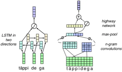
morpho-Figure 1: Model architecture for the several approaches to learning word representations, showing from left: BiLSTM over characters and the character convolution.

logically rich languages.

3 Models

Now we turn to the problem of learning word rep-resentations. We consider character level encoding methods which we compare to the baseline word embedding approach. We test two types of char-acter representations: LSTM recurrent neural net-works (RNN) and convolutional neural network (CNN).

For each type of character encoder we learn two word representations: one estimated from the characters and the word embedding.1 _{Then we}

run max pooling over both embeddings to obtain the word representation, rw = mw ew, where

mw is the embedding of word w and ew is the sub-word encoding. The max pooling operation

captures non-compositionality in the semantic meaning of a word relative to its sub-parts. We as-sume that the model would favour unit-based em-beddings for rare words and word-based for more common ones.

Each word is expressed with its constituent units as follows. LetU be the vocabulary of sub-word units, i.e., characters,Eube the dimensional-ity of unit embeddings, andM ∈REu×|U|_{be the}

matrix of unit embeddings. Suppose that a word wfrom the source dictionary is made up of a se-quence of units Uw := [u1, . . . , u|w|], where |w|

stands for the number of constituent units in the word. The resulting word representations are then fed to both attentional models as the source word embeddings.

3.1 Bidirectional LSTM Encoder

The encoding of the word is formulated using a pair of LSTMs (denoted biLSTM) one operating left-to-right over the input sequence and another operating right-to-left,h→

j =LSTM(h→j−1,muj)

andh←

j =LSTM(h←j+1,muj)whereh→j andh←j

are the LSTM hidden states.2 _{These are fed into}

perceptron with a single hidden layer and atanh

activation function to form the word representa-tion,ew= MLP

h→

|Uw|,h←1

.

3.2 Convolutional Encoder

Another word encoder we consider is a convolu-tional neural network, inspired by a similar ap-proach in language modelling (Kim et al.,2016). Let Uw ∈ REu×|U|w denote the unit-level repre-sentation ofw, where thejth column corresponds to the unit embedding of uj. The idea of unit-level CNN is to apply a kernel Ql ∈ REu×kl with the width kl to Uw to obtain a feature map

fl ∈ R|U|w−kl+1. More formally, for thejth ele-ment of the feature map the convolutional repre-sentation is

fl(j) = tanh(hUw,j,Qli+b)

where Uw,j ∈ REu×kl is a slice fromUw which spans the representations of the jth unit and its precedingkl−1units, and

hA, Bi=X

i,j

AijBij = Tr ABT

denotes the Frobenius inner product. For example, suppose that the input has size[4×9], and a kernel has size[4×3]with a sliding step being 1. Then, we obtain a[1×7]feature map. This process im-plements a charactern-gram, wherenis equal to the width of the filter. The word representation is then derived by max pooling the feature maps of the kernels:

∀l: rw(l) = max_j fl(j)

In order to capture interactions between the char-acter n-grams obtained by the filters, a highway network (Srivastava et al., 2015) is applied after the max pooling layer,

ew =tMLP(rw) + (1−t)rw, wheret = MLPσ(rw) is a sigmoid gating func-tion which modulates between atanhMLP trans-formation of the input (left component) and pre-serving the input as is (right component).

2_{The memory cells are computed as part of the recurrence,} suppressed here for clarity.

Language Ru-En Et-En

Phrase-based Baseline 15.02 24.40 AM BILSTMchar 16.01 26.34

OSM BILSTMchar 15.81 26.14

AM CNNchar 15.90 26.14

OSM CNNchar 15.94 25.97

AM BILSTMword 15.93 26.33

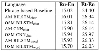
OSM BILSTMword 15.70 26.03 Table 2: BLEU scores for re-ranking the test sets.

4 Experiments

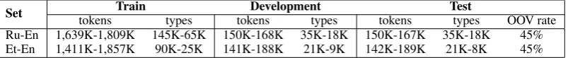
Datasets. We use parallel bilingual data from Europarl for Estonian-English (Koehn,2005), and web-crawled parallel data for Russian-English (Antonova and Misyurev,2011). For preprocess-ing, we tokenize, lower-case, and filter out sen-tences longer than 30 words. We apply a fre-quency threshold of 5, replacing low-frefre-quency words with a special UNK token. Table1presents the corpus statistics.

4.1 Extrinsic Evaluation: MT

We apply the character level models in the en-coder of the neural attentional (Bahdanau et al., 2015) (AM, soft-attentional) and neural operation sequence (Vylomova et al., 2016) (OSM, hard-attentional) models, replacing the source word em-bedding component with a BiLSTM or CNN over characters. To evaluate translations, we re-ranked moses3 _{100-best output translations using the}

at-tentional models. The re-ranker includes standard features from moses plus an extra feature(s) for each of the models. For the AM we supply the log probability of the candidate translation, and for the OSM we add two extra features correspond-ing to the generated alignment and the translation probabilities. The weights of the re-ranker are then trained using MERT (Och,2003) with 100 restarts to optimise BLEU.

Table2presents BLEU score results. As seen, re-ranking based on neural models’ scores outper-forms the phrase-based baseline. However, the translation quality of the neural models are not significantly different. We assume that this is due to re-ranking of moses translations rather than de-coding. Also note that here we do not address the problem of OOV on the decoding side.

4.2 Intrinsic Evaluation

We now take a closer look at the embeddings learned by the models, based on how well they

Set _tokensTrain _{types tokens}Development_{types tokens} Test_{types OOV rate}

Ru-En 1,639K-1,809K 145K-65K 150K-168K 35K-18K 150K-167K 35K-18K 45% Et-En 1,411K-1,857K 90K-25K 141K-188K 21K-9K 142K-189K 21K-8K 45%

Table 1: Corpus statistics for parallel data between Russian/Estonian and English. The OOV rate are the fraction of word types in the source language that are in the test set but are below the frequency cut-off or unseen in training.

capture thesemanticandmorphological informa-tion in the nearest neighbour words. Learning representations for low frequency words is harder than that for high-frequency words, since low fre-quency words cannot capitalise as reliably on their contexts. Therefore, we split the test lexicon into 6 parts according to their frequency in the train-ing set. Since we set out word frequency thresh-old to 5 for the training set, all words appearing in the lowest frequency band [0,4] are OOVs for the test set. For each word of the test set, we take its top-20 nearest neighbours from the whole training lexicon using cosine similarity.

Semantic Evaluation. We investigate how well the nearest neighbours are interchangable with a query word in the translation process. So we for-malise the notion of semantics of the source words based on their translations in the target language. We usepivotingto define the probability of a can-didate word e0 _{to be the synonym of the query}

word e, p(e0_{|e) =} P

fp(f|e)p(e0|f), wheref is a target language word, and the translation prob-abilities inside the summation are estimated using a word-based translation model trained on the en-tire initial bilingual corpora. We then take the top-5 most probable words as the gold synonyms for each query word of the test set.4

We measure the quality of predicted near-est neighbours using the multi-label accuracy5_,

1

|S| P

w∈S1[G(w)∩N(w)6=∅]whereG(w)andN(w)

are the sets of gold standard synonyms and near-est neighbors forwrespectively; the function1[C]

is one if the condition C is true, and zero other-wise. In other words, it is the fraction of words inS whose nearest neighbours and gold standard synonyms have non-empty overlap.

Table3presents the semantic evaluation results. As seen, for the vanilla (soft) attentional model word- and character-level representations perform

4_{We remove query words whose frequency is less than a} threshold in the initial bilingual corpora, since pivoting may not result in high quality synonyms for such words.

5_{We evaluated using mean reciprocal rank (MRR)} mea-sure as well, and obtained results consistent with the multi-label accuracy (omitted due to space constraints).

Model Freq. 0-4 5-9 10-14 15-19 20-50 50+

Russian

AM BILSTMword - 0.32 0.52 0.65 0.81 0.95

OSM BILSTMword - 0.36 0.49 0.61 0.76 0.91

AM BILSTMchar 0.21 0.33 0.49 0.58 0.71 0.85

OSM BILSTMchar 0.16 0.34 0.48 0.59 0.71 0.85

AM CNNchar 0.13 0.23 0.38 0.47 0.61 0.84

OSM CNNchar 0.43 0.71 0.77 0.77 0.81 0.81

Estonian

AM BILSTMword - 0.39 0.53 0.63 0.72 0.88

OSM BILSTMword - 0.48 0.62 0.70 0.79 0.90

AM BILSTMchar 0.12 0.30 0.37 0.45 0.52 0.70

OSM BILSTMchar 0.13 0.39 0.48 0.55 0.63 0.78

AM CNNchar 0.12 0.25 0.33 0.42 0.52 0.75

OSM CNNchar 0.48 0.70 0.75 0.76 0.78 0.78

Table 3: Semantic evaluation of nearest neighbours using multi-label accuracy on words in different frequency bands.

quite similar. In case of thehardattentional model we OSM CNN_char outperforms other

representa-tions by a large margin.

Morphological Evaluation. We now turn to evaluating the morphological component. We only focus on Russian since it has a notoriously hard morphology. We run another morphological anal-yser,mystem (Segalovich, 2003), to generate lin-guistically tagged morphological analyses for a word, e.g. POS tags, case, person, plurality, etc. We represent each morphological analysis with a bit vector, where each 1 bit indicates the pres-ence of a specific grammatical feature. Each word is then assigned a set of bit vectors correspond-ing to the set of its morphological analyses. As themorphology similaritybetween two words, we take the minimum of Hamming similarity6

be-tween the corresponding two sets of bit vectors. Table4(a) shows the average morphology similar-ity between the words and their nearest neighbours across the frequency bands. Likewise, we repre-sent the words based on their lemma features; Ta-ble4(b) shows the average lemma similarity.

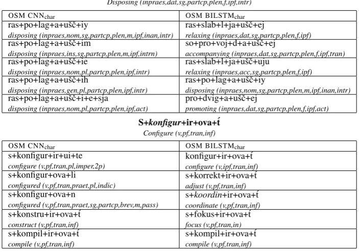
Table 5 lists top five nearest neighbours for OOV words produced by the OSM models. BiL-STMs better capture morphological similarities expressed in suffixes and prefixes. We assume this

Ras+po+lag+a+ušˇc+ej

Disposing (inpraes,dat,sg,partcp,plen,f,ipf,intr)

OSM CNNchar OSM BILSTMchar

ras+po+lag+a+ušˇc+iy

disposing (inpraes,nom,sg,partcp,plen,m,ipf,inan,intr) ras+slab+l+ja+ušˇc+ejrelaxing (inpraes,dat,sg,partcp,plen,f,ipf) ras+po+lag+a+ušˇc+im

disposing (inpraes,ins,sg,partcp,plen,m,ipf,intrn) so+pro+voj+d+a+ušˇc+ejaccompanying (inpraes,dat,sg,partcp,plen,f,ipf,tran) ras+po+lag+a+ušˇc+ie

disposing (inpraes,nom,pl,partcp,plen,ipf,intr) ras+slab+l+ja+ušˇc+ujurelaxing (inpraes,acc,sg,partcp,plen,f,ipf) ras+po+lag+a+ušˇc+ih

disposing (inpraes,gen,pl,partcp,plen,ipf,intr) ras+po+lag+a+ušˇc+iydisposing (inpraes,nom,sg,partcp,plen,m,ipf,inan,intr) ras+po+lag+a+ušˇc+i+e+sja

disposing (inpraes,nom,pl,partcp,plen,ipf,act) pro+dvig+a+ušˇc+ejpromoting (inpraes,dat,sg,partcp,plen,f,ipf,act)

S+konfigur+ir+ova+´t

Configure (v,pf,tran,inf)

OSM CNNchar OSM BILSTMchar

s+konfigur+ir+ui+te

configure (v,pf,tran,pl,imper,2p) konfigur+ir+ova+´tconfigure (v,ipf,tran,inf) s+konfigur+ova+li

configured (v,pf,tran,praet,pl,indic) s+korrekt+ir+ova+´tadjust (v,pf,tran,inf) s+konfigur+ova+n

configured (v,pf,tran,praet,sg,partcp,brev,m,pass) s+coordinate (v,pf,tran,inf)koordin+ir+ova+´t s+konstru+ir+ova+´t

construct (v,pf,tran,inf) s+fokus+ir+ova+´tfocus (v,pf,tran,in) s+kompil+ir+ova+´t

compile (v,pf,tran,inf) s+kompil+ir+ova+´tcompile (v,pf,tran,inf)

Table 5: Analysis of the five most similar Russian words (initial word is OOV), under theOSM CNNcharandOSM BILSTMchar word encodings based on cosine similarity. The diacritic ´ indicates softness.POS tags:s-noun,a-adjective,v-verb;Gender: m-masculine, f-feminine, n-neuter; Number: sg-singular, pl-plural; Case: nom-nominative,gen-genitive,dat-dative, acc -accusative,ins-instrumental,abl-prepositional,loc-locative;Tense:praes-present,inpraes-continuous,praet-past,pf-perfect, ipf-imperfect; indic-indicative; Transitivity: trans-transitive, intr-intransitive; Adjective form: br-brevity,plen-full form, poss-possessive;Comparative:supr-superlative,comp-comparative;Noun person:1p-first,2p-second,3p-third;

Model \ Freq. 0-4 5-9 10-14 15-19 20-50 50+

AM BILSTMword - 0.70 0.73 075 0.78 0.82

OSM BILSTMword - 0.74 0.77 0.78 0.81 0.84

AM BILSTMchar 0.90 0.82 0.83 0.83 0.84 0.82

OSM BILSTMchar 0.91 0.84 0.85 0.85 0.86 0.86

AM CNNchar 0.82 0.76 0.77 0.78 0.79 0.81

OSM CNNchar 0.79 0.80 0.79 0.79 0.79 0.79

(a)

Model \ Freq. 0-4 5-9 10-14 15-19 20-50 50+

AM BILSTMword - 0.02 0.04 0.07 0.11 0.18

OSM BILSTMword - 0.03 0.05 0.06 0.09 0.15

AM BILSTMchar 0.08 0.06 0.10 0.11 0.12 0.21

OSM BILSTMchar 0.05 0.05 0.08 0.10 0.13 0.18

AM CNNchar 0.04 0.02 0.05 0.06 0.1 0.15

OSM CNNchar 0.20 0.37 0.41 0.42 0.44 0.41

(b)

Table 4: Morphology analysis for nearest neighbours based on (a) Grammar tag features, and (b) Lemma features, evalu-ated on Russian.

is due to the fact that they are naturally biased towards most recent inputs. CNNs, on the other hand, are more invariant of character positions and provide whole-word similarity.

5 Conclusion

We studied two types of attentional models aug-mented by CNN and LSTM encodings. Our exper-iments demonstrate that representation of out-of-vocabulary words with their sub-word units on the

source side did not lead to a significant improve-ment in overall quality of machine translation; however LSTMs applied to character sequences are more capable at learning morphological pat-terns. Moreover, a hard attention mechanism leads to better capturing of semantic and morphological regularities.

References

Alexandra Antonova and Alexey Misyurev. 2011. Building a web-based parallel corpus and filtering out machine-translated text. InProceedings of the 4th Workshop on Building and Using Comparable Corpora: Comparable Corpora and the Web. As-sociation for Computational Linguistics, pages 136– 144.

Dzmitry Bahdanau, Kyunghyun Cho, and Yoshua Ben-gio. 2015. Neural machine translation by jointly learning to align and translate. In Proceedings of the International Conference on Learning Represen-tations (ICLR). San Diego, CA.

Miguel Ballesteros, Chris Dyer, and Noah A Smith. 2015. Improved transition-based parsing by mod-eling characters instead of words with lstms. arXiv preprint arXiv:1508.00657.

ma-chine translation models learn about morphology? arXiv preprint arXiv:1704.03471.

Jan A Botha and Phil Blunsom. 2014. Compositional morphology for word representations and language modelling. arXiv preprint arXiv:1405.4273.

Jason PC Chiu and Eric Nichols. 2015. Named en-tity recognition with bidirectional lstm-cnns. arXiv preprint arXiv:1511.08308.

Marta Costa-jussà and Jose Fonollosa. 2016. Character-based neural machine translation. arXiv preprint arXiv:1603.00810.

Mathias Creutz and Krista Lagus. 2007. Unsupervised models for morpheme segmentation and morphol-ogy learning. ACM Transactions on Speech and Language Processing (TSLP)4(1):3.

Georg Heigold, G ünter Neumann, and Josef van Gen-abith. 2017. An extensive empirical evaluation of character-based morphological tagging for 14 lan-guages. In Proceedings of the 15th Conference of the European Chapter of the Association for Com-putational Linguistics. volume 1, pages 505–513.

Sepp Hochreiter and Jürgen Schmidhuber. 1997. Long short-term memory. Neural computation 9(8):1735–1780.

Nal Kalchbrenner and Phil Blunsom. 2013. Recurrent continuous translation models. In EMNLP. pages 1700–1709.

Yoon Kim, Yacine Jernite, David Sontag, and Alexan-der Rush. 2016. Character-aware neural language models. InProceedings of the Thirtieth AAAI Con-ference on Artificial Intelligence (AAAI-16).

Yoon Kim, Yacine Jernite, David Sontag, and Alexan-der M Rush. 2015. Character-aware neural language models. arXiv preprint arXiv:1508.06615.

Philipp Koehn. 2005. Europarl: A parallel corpus for statistical machine translation. InMT summit. vol-ume 5, pages 79–86.

Guillaume Lample, Miguel Ballesteros, Sandeep Sub-ramanian, Kazuya Kawakami, and Chris Dyer. 2016. Neural architectures for named entity recognition. arXiv preprint arXiv:1603.01360.

Wang Ling, Tiago Luís, Luís Marujo, Ramón Fernan-dez Astudillo, Silvio Amir, Chris Dyer, Alan W Black, and Isabel Trancoso. 2015. Finding function in form: Compositional character models for open vocabulary word representation. arXiv preprint arXiv:1508.02096.

Thang Luong, Richard Socher, and Christopher D Manning. 2013. Better word representations with recursive neural networks for morphology. In CoNLL. Citeseer, pages 104–113.

Xuezhe Ma and Eduard Hovy. 2016. End-to-end sequence labeling via bi-directional lstm-cnns-crf. arXiv preprint arXiv:1603.01354.

Franz Josef Och. 2003. Minimum error rate training in statistical machine translation. InProceedings of the 41st Annual Meeting on Association for Compu-tational Linguistics-Volume 1. Association for Com-putational Linguistics, pages 160–167.

Cicero D. Santos and Bianca Zadrozny. 2014. Learning character-level representations for part-of-speech tagging. In Proceedings of the 31st International Conference on Machine Learning (ICML-14). pages 1818–1826.

Ilya Segalovich. 2003. A fast morphological algorithm with unknown word guessing induced by a dictio-nary for a web search engine. InMLMTA. Citeseer, pages 273–280.

Rupesh K Srivastava, Klaus Greff, and Jürgen Schmid-huber. 2015. Training very deep networks. In Ad-vances in Neural Information Processing Systems. pages 2368–2376.

Ilya Sutskever, Oriol Vinyals, and Quoc VV Le. 2014. Sequence to sequence learning with neural net-works. In Neural Information Processing Systems (NIPS). Montréal, pages 3104–3112.

Clara Vania and Adam Lopez. 2017. From characters to words to in between: Do we capture morphology? arXiv preprint arXiv:1704.08352.