Comments on Colley, Section 7.3
This section describes two 3 – dimensional generalizations of Green’s Theorem. One of them (Stokes’ Theorem) extends the usual form of Green’s Theorem involving the integral of F · ds, and the other (sometimes also called Green’s Theorem, but more often called the Divergence Theorem or Gauss’s Theorem or the Gauss – Ostrogradsky Theorem) extends the divergence form of Green’s Theorem involving the integral of F · dN.
BACKGROUND REFERENCES. The divergence and curl of a vector field were defined and studied in Section 3.4 of the text; the latter section was covered in the first course of the multivariable calculus sequence (Mathematics 10A). The following document contains some additional information and online references:
http://math.ucr.edu/~res/math10A/weblinks3.pdf
Up to this point in the course, most of the emphasis has been upon the basic definitions of key concepts (various sorts of integrals, “nice” regions in the coordinate plane and 3 – space, potential functions, surface area, flux of a vector field, … ) and methods for computing various integrals and functions, including statements of several fundamentally important theorems like the Change of Variables Rule and Green’s Theorem. While these points are also central to the remaining sections of the course, there will also be an additional factor: We shall also focus on the logical derivations of some important formulas that play crucial roles in the applications of vector analysis to the sciences and engineering.
Stokes’ Theorem
This is result which contains the previously stated Green’s Theorem (involving the line integral of F · ds over a closed curve ΓΓΓΓ, or a collection of closed curves,
bounding a region D) as a special case. The main difference is that the region D is replaced by a coherently oriented surface S. There is a discussion of coherent orientations at the end of the commentary for the previous section:
http://math.ucr.edu/~res/math10B/comments0702.pdf
The underlying ideas regarding coherent orientations are summarized in the following drawings. The first two pictures illustrate the relationship between the direction sense of ΓΓΓΓ and the orientation of S, while the third illustrates how
(Source: http://www.ittc.ku.edu/~jstiles/220/handouts/Stokes%20Theorem_1.png)
(Source: http://upload.wikimedia.org/wikipedia/commons/thumb/c/cd/Stokes.png/250px-Stokes.png)
The third picture reflects the basic principle in the previously cited commentary for Section 7.2 of the text; namely, if one has a coherent orientation for S then the sums of the line integrals over the pieces of S will reduce to the line integral over the boundary curve(s).
Yet another way of describing the relation between the orientation of S and the direction sense of the boundary curve ΓΓΓΓ is the following Right Hand Rule: If
you right hand curls around the normal vector N in the directed sense of ΓΓΓΓ, then
your thumb will be pointing in the direction of N.
With the preceding conventions, we may state Stokes’ Theorem as follows:
Let S be an oriented surface with unit coherent normal vector system N, and let ΓΓΓΓ be the positively oriented boundary of S. If F is a vector
Frequently one sees the displayed equation in an equivalent form using notational conventions such as the ∇∇∇∇ operator; here is a typical example:
There are also versions of Stokes’ Theorem for oriented surfaces whose boundaries consist of several curves; in these cases, the right hand side is replaced by a sum of line integrals over the various boundary curves, where each has the sense it inherits from the coherent orientation system for the surface.
On the other hand, Stokes’ Theorem does not apply to the Möbius strip discussed in the commentary for Section 7.2; as indicated there, the sum of the line integrals over the parametrized pieces is never equal to the line integral along the boundary. No matter which orientation system one chooses for the parametrized pieces of the Möbius strip, the sum of the line integrals will always contain an extra term given by twice a line integral over a curve which is not contained in the boundary of the surface.
A computational example. This is taken from the following online source:
http://ltcconline.net/greenl/courses/202/vectorIntegration/stokesTheorem.htm
Let S be the part of the plane z = 4 – x – 2y in the first octant, with upwardly pointing unit normal vector. Use Stokes' theorem to find
SOLUTION. We first notice that, without Stokes’ theorem, it would be
necessary to parametrize three different line segments. Instead, we can evaluate the line integral by means of just one double integral. The first step is to find a suitable parametrization for the solid triangle, including the domain on which this parametrization is defined. The graph parametrization (x, y, 4 – x – 2y) will be fine for our purposes, and its domain of definition is the “shadow” that S casts upon the xy – plane, which is just the region in the first quadrant bounded by the coordinate axes and the line x + 2y = 4. We then have
and N = i + 2j + k, so that Curl F · N = 1 + x + 2y - 1 = x + 2y. Therefore the line integral in the problem is given by
and from this one sees that the value of the integral is 32/3.
More conceptual implications of Stokes’ Theorem
On a theoretical level¸ one important consequence of Stokes’ Theorem is its role in proving a fundamental result from Theorem 6.3; namely, a vector field F over a simply connected region ΩΩΩΩ in 3 – dimensional space is expressible the gradient ∇
∇ ∇
∇g of some function g on ΩΩΩΩ if and only if ∇∇∇∇× F = 0. Here is a brief sketch of
how one derives this fact. Let p be some fixed point in ΩΩΩΩ, for each x in the
region pick some simple piecewise smooth path ΓΓΓΓ joining p to x, and set g(x)
equal to the line integral of F over ΓΓΓΓ. . . . In order to justify this definition, one needs
to check that it does not depend upon the choice of smooth path; this turns out to be a consequence of the simple connectivity hypothesis, the vanishing of the curl, and Stokes’ Theorem. Given this, one can verify that ∇∇∇∇g = F fairly directly.
On a qualitative computational level, Stokes’ Theorem is useful because it often allows a priori evaluation of integrals without doing explicit quantitative
computations.
Example. Suppose that S is the boundary of the cube defined by the inequalities – 1 ≤ x, y, z ≤ 1, and assume that F is a vector field defined near S. Prove that
SOLUTION. The surface integral is a sum of the surface integrals over the six flat pieces (as in the commentary for Section 7.2).
(Source: http://rationalwiki.com/wiki/images/2/20/400px-Necker_cube.svg.png)
By Stokes’ Theorem, the integral of ∇∇∇∇× F over each piece of S is equal to the
Same cube as before, with arrows indicating the senses of some line integrals over edges
The sense of the boundary curve for the front face of the cube (mathematically, the face defined by y = – 1) is indicated by the red arrows, and the senses of the four adjacent faces are indicated by the arrows in contrasting colors. Notice that each piece of a boundary curve marked with a red arrow corresponds to another curve which has the opposite sense and is marked with an arrow of a different color. This means that if one sums up the line integrals over all the boundary pieces of the surface S, then the net result will not contain any terms involving the boundary curves over the front face. By the symmetry of the cube, the same is true for every other face, and therefore the sum of the line integrals of the boundary curves for all six faces will be equal to zero.
This is just a special case of a more general phenomenon. If we have an oriented surface with no boundary curves given in terms of pieces, then for a coherent system of orientations the sums of the line integrals for all the properly sensed boundary curves will be equal to zero. In particular, this also applies to objects like cylinders (whose pieces are the tops, bottoms, and lateral faces) or spheres. Thus the vanishing result for cube surfaces also holds for an arbitrary surface with no boundary curves.
Note that the vector field need not be defined over the entire solid cube which is bounded by S; for example, this formula applies to the “inverse square” vector field sending a vector v = (x, y, z) to |v|– 3 v (same direction as v, but the length is equal to |v|– 2).
Derivation of Stokes’ Theorem
g(x) ≤ y ≤ h(x). This turns out to be a direct consequence of the “easy special case” of Green’s Theorem for such regions combined with the definitions of line and flux integrals. The second step is to view a general surface as a union of pieces to which the first step applies. Then we know that the total surface integral is equal to the sum of the surface integrals over the pieces, so by the special cases it is equal to a sum of line integrals over the boundary curves for these pieces. But the orientability condition implies that the sum of the line integrals over all the boundary curves for the pieces is just the line integral over the boundary of the whole surface (if the boundary consists of several closed curves, then one must take the sum of the line integrals over all the boundary curves). Therefore the line integral of F over the boundary curve (or the sum of these curves) is equal to the surface integral for the curl of F over the entire surface. Some further
information and additional details appear on pages 448 – 451 of the course text.
The Divergence Theorem
The second generalization of Green’s Theorem to 3 – dimensional space, often known as the Divergence Theorem, is an analog of the Green’s Theorem identity for flux integrals (line integral of flux equals double integral of the divergence over the region bounded by the curve or curves).
Let V be a region in coordinate 3 – space which lies inside some large cube, and assume that the boundary of V is a piecewise smooth surface S (which, by previous comments, has a coherent orientation system N), and take the outward pointing orientation of S. Assume further that F is a vector field with continuous first order partial derivatives which is defined in a region containing V. Then we have the following identity:
This result is closely related to the physical interpretation of the divergence which is mentioned in Chapter 3 of the text: Namely, if F is the velocity vector field for fluid motion in some region at a specific time, then the value of the divergence function ∇∇∇∇· F(p) at some point p measures the extent to which the fluid is
expanding or contracting at p. If one thinks of the fluid as the atmosphere, then the divergence of F indicates whether the barometric pressure is rising (negative divergence) or falling (positive divergence) by Boyle’s Law (the pressure and volume of a gas are inversely proportional to each other if the temperature is held constant).
A computational example. This is taken from the following online source:
http://en.wikipedia.org/wiki/Divergence_theorem
Find the flux of the vector field F(x, y, z) = (2x, y2, z2) over the unit sphere with the outward normal orientation.
SOLUTION. Direct computation of this integral is turns out to be fairly difficult, but we can evaluate the surface integral fairly easily by means of the Divergence Theorem because the vector field is defined on the unit disk W whose boundary is the sphere S. If we apply this theorem, we obtain the following:
Since the functions y and z are odd functions on the surface S — in other words, they satisfy F(– x, – y, – z) = – F(x, y, z) for all (x, y, z) — and the surface S is symmetric with respect to the antipodal map sending (x, y, z) to ( – x, – y, – z), we automatically have
because the unit disk W bounded by S has volume equal to 4ππππ/3.
The Divergence Theorem is also useful for computing surface integrals when the boundaries of surfaces are somewhat complicated. In particular, the example below is worked out in the following document:
http://math.ucr.edu/~math10B/divthm.pdf
Let S be the boundary of the region defined by the xy – plane, the right circular cylinder x 2 + y 2 = 4, and the plane x + z = 6. Take the outward normal orientation on S. Compute the flux of the vector field
F(x, y, z) = (x 2 + sin z, xy + cos z, ey)
over the surface S. A drawing of the surface is given below.
More conceptual implications of the Divergence Theorem
As in the case of Stokes’ Theorem, the Divergence Theorem also has several noteworthy consequences of a qualitative nature.
Volume computations. We have already noted that Green’s Theorem provides ways of computing the area of a “good” region D in the coordinate plane by means of line integrals over its boundary curve ΓΓΓΓ. There are similar formulas for
computing the volumes of “good” regions D in coordinate 3 – space by means of surface integrals over their boundary surfaces S. In the planar case, the key was to find vector fields F = (P, Q) such that Q1 – P2 = 1. Similarly, in the 3 –
dimensional case, the key is to find vector fields F such that ∇∇∇∇· F = 1. Some
obvious choices are the vector fields (x, 0, 0), (0, y, 0), and (0, 0, z). For these choices, the Divergence Theorem yields the following volume formulas:
Of course, the volume is also equal to the average of the three surface integrals on the right hand side, and hence the volume is also equal to
which is also one third the flux of the “identity” vector field F(x, y, z) = (x, y, z).
Another basic source of examination problems are the “bait and switch” examples in which one has a vector field F with ∇∇∇∇· F = 0. One problem of this sort
Let S be the boundary of the region in the half – space z ≥ 0 defined by the spheroid with equation x 2 + y 2 + 2z 2 = 1, and take the outward normal orientation on S. Compute the flux of the vector field
F(x, y, z) = (y, z, x)
over the surface S.
We first note that the divergence of F vanishes. In a previous document we defined a parametrization for S; one indication that the surface integral computation might be complicated is that the given parametrization involves SQRT(2) as a coefficient.
The key observation in a problem of this sort is that the flux integral over S is equal to the flux integral over the flat disk S′ (with the upward normal).
To see this, note that S with the outward normal and S′ with the downward normal form the boundary of the oblate hemispherical region defined by the inequalities z ≥ 0 and x 2 + y 2 + 2z 2 ≤ 1, Since the surface integral of S′ with the downward normal and the S′ with the upward normal are negatives of each other, it follows that
Solving the vector field equation F =
∇
∇
∇
∇
×
G for G
In Chapter 6 of the course text we considered the question of whether a given vector field F can be expressed as the gradient ∇∇∇∇g of some function g. As
noted earlier in this document and other commentaries, the condition ∇∇∇∇× F = 0
is always a necessary condition (since the curl of a gradient is always zero), and if the region is suitably restricted this condition is also sufficient. Something similar happens with 3 – dimensional vector fields and the curl operator. One can check directly that ∇∇∇∇· (∇∇∇∇× F) vanishes for all choices of F. Moreover, if the region is
suitably restriced (for example, the region is all of 3 – space), then it turns out that F = ∇∇∇∇× G for some vector field G
if and only if ∇∇∇∇· F = 0; we should note that the simple connectivity condition which appears in the theorem on recognizing gradients is not the appropriate restriction in the theorem on recognizing curls.
We shall conclude this commentary with an example of a vector field F defined over all points of 3 – space except the origin such that ∇∇∇∇· F = 0 but F is not
the curl of a vector field defined everywhere in this region of space. We shall take F to be the “inverse square” vector field sending a nonzero vector v = (x, y, z) to F(v) = |v|– 3 v (same direction as v, but the length is equal to |v|– 2). By Exercise 19 on page 222 of the course text, we know that ∇∇∇∇· F = 0.
On the other hand, if S is the unit sphere in coordinate 3 – space, then the
integrand of the flux integral is F · N = 1, and therefore the flux of F over S is equal to the surface area of S, which is 4ππππ. Using this, we can show that F is not
the curl ∇∇∇∇× G of some vector field G as follows: If F = ∇∇∇∇× G on some
region containing all points sufficiently close to S, then by Stokes’ Theorem it follows that the surface integral of F over S must be zero, for the surface S has no boundary curves. Since we know that the flux of F over S is nonzero, it follows that the vector field F cannot be the curl of some other vector field G defined on all points sufficiently close to the sphere S.
Derivation of the Divergence Theorem
Not surprisingly, this is much like the arguments we discussed for verifying
threefold iterated integrals; specifically, these are regions defined by standard sequences of inequalities like the following:
a ≤ x ≤ b, g(x) ≤ y ≤ h(x), u1(x, y) ≤ z ≤ u2(x, y)
Here is a drawing of a typical example, in which D corresponds to the region defined by inequalities of the form a ≤ x ≤ b and g(x) ≤ y ≤ h(x).
(Source: http://tutorial.math.lamar.edu/Classes/CalcIII/TripleIntegrals.aspx)
As in the case of Green’s Theorem, verifying the Divergence Theorem for this special case is merely a matter of writing down the surface integral and the triple integral and then checking that these integrals are in fact equal; informally
speaking, we may describe this as “an exercise in bookkeeping.”
The second step is to show that the Divergence Theorem is also true if the surface and bounding region are obtained from the preceding standard examples by a “good” change of variables transformation (x, y, z) = T(u, v, w) of the sort considered in Section 5.5 of the course text; in other words, the mapping T is supposed to be one – to – one and onto, its three coordinate functions x(u, v, w), y(u, v, w), and z(u, v, w) are supposed to have continuous first partial derivatives, and the Jacobian of (x, y, z) with respect to (u, v, w) is never equal to zero.
A typical example is shown in the drawing below; the idea is that the change of variables transformation T maps the solid rectangular box on the left to the box on the right with curved edges and faces.
If we have a transformation T defined on a tetrahedral region as illustrated above, then we get a similar picture.
The third step is intuitively fairly simple, but it is also extremely difficult to prove rigorously. Namely, we need to show that if we are given an arbitrary region D bounded by a piecwise smooth surface (or configuration of surfaces), then it can be expressed as a union of nonoverlapping regions Dk of the sort considered in the second step. One then checks that the triple integral over D is the sum of the triple integrals over the subregions , and similarly the surface integral over the boundary S is equal to the sum of the surface integrals over the boundaries Sk of the subregions Dk. Since the appropriate integrals over the regions Dk and
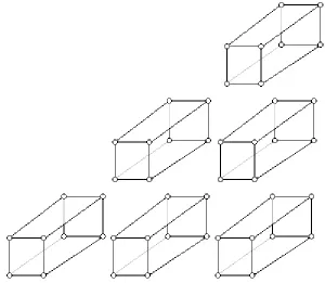
Here is a simple example which illustrates the final part of the argument. The figure below may be viewed as a solid staircase with three steps; its boundary consists of the steps, the right hand side, the front and the back.
(Source: http://www.tiffinmats.com/html/images/stairSteps.jpg)
This figure is equal to a union of six rectangular boxes which are stacked as indicated in the drawing below.