Online Full Text

(1)

Abstract—This research investigated numerical solutions of generalized variable order fractional partial differential equations by using Bernstein polynomials. In addition, the Caputo differential derivative was adopted. Among fractional operational matrices, which contained x or t, of Bernstein polynomials were derived and utilized to transform the initial equation into the solution of algebraic equations after dispersing the variable. By solving algebraic equations, numerical solutions were acquired. The method, in general, is easy to implement and yields good results. Numerical examples are provided to demonstrate the validity and applicability of the method.

Index Terms—Bernstein polynomials; generalized variable order fractional differential equation; operational matrix; numerical solution; convergence analysis

I. INTRODUCTION

RACTIONAL differential equations, advantageous due to their capability of simulating natural physical process and more accurate dynamic system, are obtained by replacing integer order derivatives with fractional ones[1, 2]. In general, it is difficult to derive analytical solutions for most fractional differential equations. Therefore, it is important to develop reliable and efficient techniques to solve fractional differential equations. The most commonly used techniques are Variational Iteration Method [3, 4], Adomian Decomposition Method [5], Block pulse function method [6], Wavelet method [7], and other methods [8-11].

In recent years, numerous researchers have found many important dynamic problems exhibit fractional order behaviour, which may be related to space and time. It is an evident fact that illustrates variable order calculus provides effective mathematical framework for complex dynamic phenomena. The concept of a variable order operator is new in science. Regarding variable order differential operators, various authors created different definitions with specific meanings to suit desired goals. Variable order operator definitions are classified by the following: Riemann-Liouvile

Manuscript received February 20, 2016; revised May 12, 2016. Hao Song is with the School of Aeronautic Science and Engineering, Beihang University, Beijing, P.R.China (e-mail: [email protected]).

Mingxu Yi (Corresponding author) is with the School of Aeronautic Science and Engineering, Beihang University, Beijing, P.R.China (e-mail: [email protected]).

Jun Huang is with the School of Aeronautic Science and Engineering, Beihang University, Beijing, P.R.China

Yalin Pan is with the School of Aeronautic Science and Engineering, Beihang University, Beijing, P.R.China

definition, Caputo definition, Marchaud definition, Coimbra definition and Grünwald definition [12-17].

Since the kernel of variable order operators is they have a variable-exponent, numerical solutions of variable order fractional differential equations are quite difficult to obtain, therefore not attracting much attention. To the best of the authors’ knowledge, few references addressed the discussion of numerical variable order fractional differential equations.

This research investigated the numerical solution of the variable order fractional partial equation with Bernstein polynomials. Given its simple structure and perfect properties [18-20], Bernstein polynomials play a vital role in computational mathematics. These polynomials have been widely applied in finding solutions for fractional equations [18-25].

Similar to the classical fractional partial differential equation [26], this study focused on a class of generalised variable order fractional partial differential equation, as follows:

( )

(

( ) ( )

)

( )

(

( ) ( )

)

( )

[ ] [

] [ ]

1 2

, , , , , ,

, 0, 0, .

x t

D u x t k x t D u x t k x t f x t

x t X T

α ₊ β ₌

∈ × (1) Subject to the initial conditions:

( )

[

]

( )

[ ]

,0 0,

0, t 0, .

u x g x x X

u h t t T

= ∈

(2)

where Dα( )x

(

u x t k x t

( ) ( )

, ₁ ,

)

and Dβ( )t

(

u x t k

( ) ( )

, ₂ x t,

)

are fractional derivatives of Caputo sense. Whenu x t

( )

, =k1

( )

x t, oru x t

( )

, =k2

( )

x t, , the initial problem

was changed to a nonlinear equation.

( ) ( ) ( ) ( )

, , 1 , , 2 , , ,

f x t k x t k x t u x t were assumed to be casual

functions of time and space on the domain

( )

x t, ∈

[

0,X

] [ ]

× 0,T .f x t k

( ) ( ) ( )

, , 1 x t k, , 2 x t, was known

andu x t

( )

, was the unknown,0<α

( ) ( )

x ,β t ≤1.

This research paper is organized as follows: Section 2 provides basic definitions and properties of the variable order fractional order calculus. Section 3 explains the definition of Bernstein polynomials and function approximation. Section 4 derives fractional operational matrices of Bernstein polynomials, which were utilised to solve the equation provided. Section 5 presented numerical examples to demonstrate the efficiency of the proposed method. Section 6 summarised concluding remarks.

Bernstein Polynomials Method for a Class of

Generalized Variable Order Fractional

Differential Equations

Hao Song, Mingxu Yi*, Jun Huang, and Yalin Pan

F

IAENG International Journal of Applied Mathematics, 46:4, IJAM_46_4_05

(2)

II. BASIC DEFINITIONS AND PROPERTIES OF VARIABLE

ORDER FRACTIONAL INTEGRALS AND DERIVATIVES

This section provides basic definitions and properties of variable order fractional order calculus [12-17].

(1) Riemann-Liouville fractional integral with orderα

( )

t

( )

(

)

(

)

( )

(

)

1 1 ,

0 Re 0 .

t t

t

a _a

I u t t T u T dT

t t t α α α α −

+ =_Γ ₊ −

 

> _ > _

∫

(3)

(2) Riemann-Liouville fractional derivate with orderα

( )

t

( )

(

)

(

)

( )

1 1 , 1 . m _t t

a m a t m

u d

D u t d

dt

m t t

m t m

α α t t α t α

+ =_Γ ₋ − +

− − ≤ <

∫

₍₄₎

(3) Caputo’s fractional derivate with orderα

( )

t

( )

(

)

(

)

( )

( ) ( )

(

)

( )

(

)

0 1 1 0 0 . 1 t t t t

D u t t u d

t

u u t

t

α α

α

t t t

α α − + − ′ = − Γ − + − − + Γ −

∫

(5)

where0<α

( )

t ≤1. If the starting time is assumed to be in a perfect situation, the definition is as follows:

( )

(

)

(

)

( )

0 1 , 1 0 1. t t t

D u t t u d

t

α

α _t _{t t}

α α − + ′ = − Γ − < <

∫

₍₆₎

Generally, (6) is adopted as the definition of fractional derivate in Captuo sense.

Given the aforementioned definition, the formula is as

follows

(

0<α

( )

t ≤1

)

:

( )

(

)

( )

(

)

( )

0 0

1

1, 2,3 . 1 t a t D x x t α β β β β β β α − ∗ = 

 _Γ ₊

=  ₌

Γ + −

 

(7)

III. BERNSTEIN POLYNOMIALS AND THEIR PROPERTIES

A. Basis for the Definition of Bernstein Polynomials

The Bernstein Polynomials of degreenin

[ ]

0,R are defined by the formula:

( )

(

)

, .

n i i

i n n

n x R x

B x i R − −   =  

  (8) By using the binomial expansion of

(

R−x

)

n k− , (8) can be expressed as:

( )

(

)

( )

,

0

1 .

n i k

i n i i k

i n n i k

k

n x R x n n i x

B x

i R i k R

− ₋ ₊ + = − −      =_{ } = − _{ } _

 

∑

   (9)

Furthermore, the following is defined:

( )

0,

( )

, 1,

( )

, , ,

( )

.

T

n n n n

x = _B x B x B x _

Φ (10) where

( )

x = n

( )

x .

Φ AT (11) where

( )

0 1 0 1 0 1 0 1 0 0 1 1 1 1

0 0 1

1 1 0 1 1 0 0 0 0 1 1 0 0 1 1 1 . 1 1 1 1 n n n n n

n n n

R R n n R n n n R n n n R n n R − − −  ₋   ₋                 _{ } ₋ _ =  − _{ } _        −     − _{ } _ _ −    _  −    _ − _{ } _ −          − _{ }             A (12)

( )

2

1, , , , n T.

n x =  x x  x 

T (13) It is obvious that

( )

1

( )

.

n x x

− =

T A Φ (14) B. Function Approximation

Suppose 2

0, f , f

f∈L _ t _ t ∈R ,

let Y=Span B{ _0,_n,B_1,_n,B_2,_n,B_{n n}_, } be the set of Bernstein Polynomials of n th degree. Letf be an arbitrary element inY . SinceY is a finite dimensional vector space, fhas a unique

best approximation from Y . That

is,∃ ∀ ∈y0, y Y, f−y0 2≤ f −y2, where f 2= f f, .

Sincey0∈Y, there exist unique coefficients c c0, ,1,cnsuch

that

, , .

T

f

=

c Φ Φ Φ

(15)

where

( ) ( )

0, 1, ,

0

, tf T , , , , , .

n n n n

f Φ =

∫

f t Φ t dt=  f B f B  f B _ (16) And Φ

( ) ( )

t ,Φ t is an

(

n+ ×1

) (

n+1

)

matrix which is said to be the dual matrix of Φ, denoted byQ. Therefore,

( ) ( )

0

, tf T .

t t t t dt

= =

∫

Q Φ Φ Φ Φ (17) And

( ) ( )

(

)

1

0 .

f t

T T

f t t dt −

=

∫

c Φ Q (18) The function

( )

2

(

[

] [ ]

)

, 0, 0,

u x t ∈L X × T is approximated as

follows:

( )

, ,

( ) ( )

,

( )

0 0 , . n n T

i j i n j n

i j

u x t u B x B t x t

= =

=

∑∑

. Φ UΦ (19)

where

00 01 0

10 11 1

0 1

.

n

n n nn

u u u

      =             

U (20)

And Ucan be obtained as the following:

( )

(

( ) ( )

)

(

)

1 1

, , , .

x t u x t

− −

=

U Q Φ Φ Q (21)

IAENG International Journal of Applied Mathematics, 46:4, IJAM_46_4_05

(3)

(

)

2 3 2 2 2 . 1 ! 2 3

m T MS f c m m + − ≤ + +

Φ (21)

where ( 1)

( )

{

}

[0, ] 0 0

max , max ,

f m

t t f

M= _∈ f + t S= t −t t .

Proof: Consider Taylor polynomials

( )

( )(

)

( ) (

)

( )

( ) (

)

1 0 0 0

2 0 0 0 0 2 ! m m

f t f t f t t t

t t t t

f t f t

m ′ = + − − − ′′ + ++

which it is known

( )

( ) (

)

(

)

( )

1

1 0

1 , 0, .

1 !

m m

f

t t

f t f t f t

m ε ε + + − − = ∃ ∈ + since T

( )

c Φ t is the best approximation off , so

( )

(

)

( )

( ) (

)

(

)

(

)

(

)

(

) (

)

2 2 2

12 1

2 0 2 1 1 0 0 2 2 2 0 2 ₀

2 2 3

2

1 !

2

. 1 ! 2 3

f f f t T m t _m t m m

f c f f f t f t dt

t t

f dt

m

M

t t dx

m M S m m ε + + + + − ≤ − = −  ₋    = _ _ +   ≤ − +     ≤ + +    

∫

Φ

Taking square roots provides the above bound.

IV. ANALYSIS OF THE NUMERICAL METHOD

Consider (1). If the function u x t k

( ) ( ) ( )

, , 1 x t k, , 2 x t, is

approximated with the basis of Bernstein Polynomials, it can

be written

as

( )

, T

( )

u x t =Φ x UΦ t ,

( )

1 , 1 , 2 , 2

T T

k x t =Φ x KΦ t k x t =Φ x KΦ t , where only Uis unknown, then

( )

( ) ( )

( )

( ) ( )

( )

( ) ( )

( )

(

( )

)

( )

(

( )

)

( )

( ) 1 1 1

1 1 1

1 , , 1 1 1 x

x T T T

x

T T T

T x T T n n T x

T T T

n n

x

T T n T

n

x

T T

D u x t k x t

D t x x t

t D x x t

t

t D t t t

t t t t t D α α α α α α α ∗ ∗ ∗ ∗       = _ _   = _ _   = __ __   = _ _         _{  } _ = _ _ __      _{ }    =   

Φ U Φ Φ KΦ

Φ U A T A T KΦ

Φ U A T T A KΦ

Φ U A A KΦ

Φ U A

( )

2 1

1 1

1 2

1 1 1 .

n T

n n n

T T T

t t

t

t t t

t t + +             =      

A KΦ

Φ U A MA KΦ

(23) where

( )

0 1 0 1 0 1 1 0 1 0 0 1 1 1 1

0 0 1

1 1 0 1 1 0 0 0 0 1 1 0 0 1 1 1 . 1 1 1 1 n n n n n

n n n

X X n n X n n n X n n n X n n X − − −  ₋   ₋                 _{ } ₋ _ =  − _{ } _        −     − _{ } _ _ −    _  −    _ − _{ } _ −          − _{ }             A (24)

( )

(

)

( )

(

)

( )

(

( )

)

( )

(

)

( )

(

)

( )

(

)

( )

)

( )

(

)

( )

(

)

( )

(

)

( )

(

)

( )

(

)

( )

(

)

( ) 1 1 2 1 1 2 2 0 2 2 3 2 3 1 2 1 2 1 1 2 2 . 2 1 2 1 x x x

n x n x

n x n x n x t x t t x x n n t t

n x n x

n t n x n t n x n t n x α α α α α α α α α α α α α α α α − − − − + − − + − − Γ 

 _{Γ −}



 _Γ _Γ



 Γ − Γ −

=  

 _Γ ₊ _Γ ₊



 Γ + − Γ + −



Γ + 



Γ + − _



Γ + _



Γ + −

  

Γ + _



Γ + − _

       M

(25) Also, ( )

( ) ( )

( )

( ) ( )

( )

( ) ( )

( )

(

( )

)

( )

(

( )

)

( )

( ) 2 2 2

2 2 2

2 , , 1 1 1 t

t T T T

t

T T T

T t T T n n T t

T T T

n n

t

T n T T

n

t T

D u x t k x t

D x t t x

x D t t x

t

x D t t x

t t t t t x D β β β β β β β ∗ ∗ ∗ ∗       = _ _   = _ _   = __ __   = __ __       _{  } _ = _ _ __      _{ }    =   

Φ UΦ Φ K Φ

Φ U Φ Φ K Φ

Φ U A T A T K Φ

Φ UA T T A K Φ

Φ UA A K Φ

Φ UA

( )

2 1

2 2

2 2 2 .

n

T T

n n n

T T T

t

x

t t t

x x +             =      

A K Φ

Φ UA NA K Φ

(26)

where

IAENG International Journal of Applied Mathematics, 46:4, IJAM_46_4_05

(4)

( )

0 1

0

2 1

0

1

0

1 1

0 0 1

1 1

0 1

1 0

0 0

0 1 1

0 0

1 1 1

.

1 1

n

n n n

T T

n n

T

n n

n T

n n

n T

n n T

−

− −

 ₋   ₋   

     

    



 _{ } ₋ _

=  − _{ } _

   

  

− 

  

− _{ } _ _

−

   _

 −

   _

− _{ } _

− 

  

    

− _{ } 



  



  





A

(27)

( )

(

)

( )

(

)

( )

(

( )

)

( )

(

)

( )

(

)

( )

(

)

( )

)

( )

(

)

( )

(

)

( )

(

)

( )

(

)

( )

(

)

( )

(

)

( )

1

1 2

1

2

2 0

2

2 3

1 2

1 1

2

2 .

2 1 2 1

t

t t

n t n t

n t

t t

n n

t t

n t n t

n t

β

β β

α β

β β

β

β β

β

−

− −

− + −

−

+ −

− Γ



 _{Γ −}



 _Γ _Γ



 Γ − Γ −

=  

 _Γ ₊ _Γ ₊



 Γ + − Γ + −



Γ + 



Γ + − _



Γ + _



Γ + −

  

Γ + _



Γ + − _

 



 



N

(28)

M,Nare the fractional operational matrices which contain the variablex or t with Bernstein polynomials.

So the initial equation is transformed to the following:

( )

1 1 1 2 2 2

, .

T T T T T T

t t x x

f x t

+

=

Φ U A MA KΦ Φ UA NA K Φ

(29) Dispersing (29) with

(

x t_i, _j

)

,

(

i=1, 2,,n_x;j=1, 2,,n_t

)

using Mathematica 9.0U is obtained. Thus, the numerical solution of the original problem is ultimately obtained.

V. NUMERICAL EXAMPLES

To demonstrate the efficiency and practicability of the proposed method, the following examples are presented and related solutions were found through the method described in Section 4.

Example 1:

( )

[ ] [ ] [ ]

( )

3 2

2 2

, , , ,

, 0, 2 0,3 , ,0 , 0, .

t x

D u x t x D u x t t f x t

x t u x x u t t

+ =

   

   

∈ × = =

where

( )

(

)(

)

(

)(

)

(

)(

)

(

)(

)

1

2 2

3

1 ₂ ₂

2

3 54 9 6

,

9 6 3 1

3

2 6 4 24

.

6 4 2 1

2

t

x

t t t t x

f x t

t

t t t

x t x x x

x

x x x

−

 + − − 

 

= −

 

− − − Γ −_ _

 

 − − + 

 

−

 

− − − Γ −_ _

 

.

The exact solution of the above equation is

( )

2 2

,

u x t =x +t . The problem was solved by adopting the technique described in Section 4 using Mathematica 9.0.

Taking n=2 ,

dispersing 1, 1

(

1, 2,3; 1, 2,3

)

3 6 3 6

j i

i j i j

k k

x = − t = − k = k = , the

matrixUis displayed as follows:

1 0 0

4 1 0 0 .

4 1 1 13 9 9 36

 

 

 

U =

The numerical solution isu x t

( )

, =Φ

( )

x UΦ

( )

t , as matrixUis given above, and

( ) (

)

(

)

( ) (

)

(

)

2 ₂

2 2

2 2 2 ,

3 2 3 .

T

x x x x x

t t t t t

 

=_ − − _

 

=_ − − _

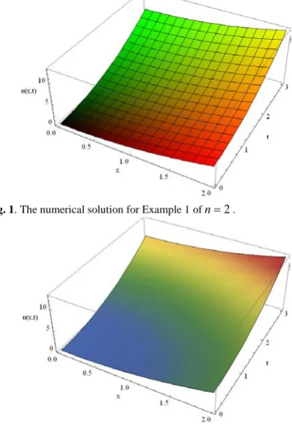
Φ

The numerical solution for n=2and the exact solution are shown in Figure 1 and Figure 2, respectively. The absolute errors between the numerical solution and exact solution are displayed in Figure 3.

Fig. 1. The numerical solution for Example 1 ofn=2.

IAENG International Journal of Applied Mathematics, 46:4, IJAM_46_4_05

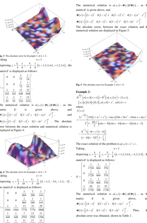
[image:4.595.51.502.46.440.2] [image:4.595.314.524.436.745.2]

(5)

Fig. 3. The absolute error for Example 1 ofn=2_.

Taking n=3 ,

dispersing 1, 1

(

1, 2,3, 4; 1, 2,3, 4

)

4 8 4 8

j i

i j i j

k k

x = − t = − k = k = , the

1 1 0 0

72 24 1 1 0 0

72 24 1 1 13 31 162 162 648 648

1 1 7 13

54 54 216 216

 

 

=  

 

 

U .

The numerical solution is u x t

( )

, =Φ

( )

x UΦ

( )

t , as the

matrix U is given above, and

( ) (

)

3

(

)

2

(

)

2 3

2 3 2 3 2 ,

T

x =_ −x −x x −x x x _

Φ and

( ) (

)

3

(

)

2

(

)

2 3

3 3 3 3 3

T

t =_ −t −t t −t t t _

Φ . The absolute

error between the exact solution and numerical solution is displayed in Figure 4:

Taking n=4 ,

dispersing 1, 1

(

1, 2, 5; 1, 2, 5

)

5 10 5 10

j i

i j i j

k k

x = − t = − k =  k =  ,

the matrixUis displayed as follows:

1 1 1

0 0

864 288 144

1 1 1

0 0

864 288 144

1 1 13 31 29

. 1944 1944 7776 7776 3888

1 1 7 13 11

648 648 2592 2592 1296

1 1 11 17 13

324 324 2592 2592 1296

 

 

=

 

 

U

( )

, =Φ

( )

x UΦ

( )

t , as the matrixUis given above, and

( ) (

)

(

)

(

)

(

)

( ) (

)

(

)

(

)

(

)

4 3 2 2 3 4

1 4 2 6 2 4 2 ,

3 4 3 6 3 4 3 .

T

x x x x x x x x x

t t t t t t t t t

 

=_ − − − − _

 

=_ − − − − _

Φ

The absolute errors between the exact solution and the numerical solution are displayed in Figure 5.

Example 2:

( )(

)

( )

[ ] [ ] [ ]

( )

sin

3 2

3

, , , ,

, 0, 4 0,3 , ,0 , 0, .

t x

D u x t x t D u x t xt f x t

x t u x x u t t

+ + =

   

   

∈ × = =

where

( )

(

)

(

)

(

)(

)

(

)

(

)(

)

sin 1

2 3 2 2

2

1 ₃

3

2 192 sin 104 24 18sin sin sin

1 sin 8 sin 6 sin 4 sin 2 2

3 6

,

6 .

6 3 1

3

x

t

x t tx x t x x x x

x

x x x x

t x t x t

t

t t

f x t

−

 + + − + − + 

 

 

Γ −_ _ − − − −

 

− + − 

 

−

 

− − Γ −_ _

 

=

The exact solution of the problem is

( )

3

,

u x t =x +t.

Taking n=3 ,

dispersing 1, 1

(

1, 2,3, 4; 1, 2,3, 4

)

4 8 4 8

j i

i j i j

k k

x = − t = − k = k = , the

1 1 1

0

1728 864 576

1 1 1

0

1728 864 576

1 1 1

0

1728 864 576 1 65 11 67 27 1728 288 1728

 

 

=  

 

 

U

( )

, =Φ

( )

x UΦ

( )

t , as the

matrix U is given above, and

( ) (

)

3

(

)

2

(

)

2 3

4 3 2 3 4 T,

x =_ −x −x x −x x x _

Φ

( ) (

)

3

(

)

2

(

)

2 3

3 3 3 3 3 .

T

t =_ −t −t t −t t t _

Φ Thus, the

absolute error was obtained, shown in TableⅠ.

IAENG International Journal of Applied Mathematics, 46:4, IJAM_46_4_05

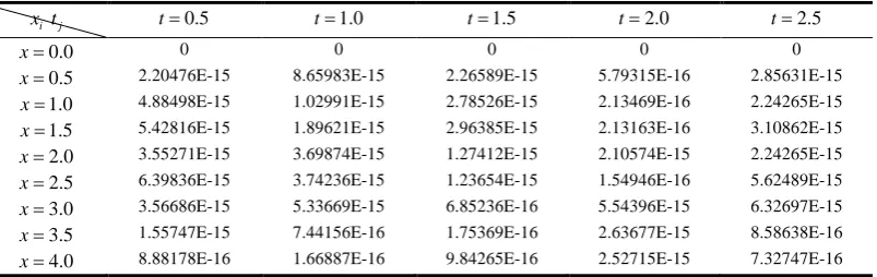
[image:5.595.52.541.40.778.2] [image:5.595.49.286.44.457.2] [image:5.595.319.526.149.318.2]

(6)

Taking n=4 ,

dispersing 1, 1

(

1, 2, 5; 1, 2, 5

)

5 10 5 10

j i

i j i j

k k

x = − t = − k =  k =  ,

the matrixUis displayed as follows:

1 1 1 1

0

27648 13824 9216 6912

1 1 1 1

0

27648 13824 9216 6912

1 1 1 1

0

27648 13824 9216 6912

1 67 35 73 19

1296 82944 41472 82944 20736 1 259 131 265 67 324 82944 41472 82944 20736

 

 

=

 

 

U

The absolute error was obtained, shown in Table Ⅱ. Example 3:

( )

[ ] [ ] [ ]

( )

2 2

3 2

2 2

, , , ,

, 0, 2 0, 2 , ,0 , 0, .

x t

D u x t D u x t f x t

x t u x x u t t

 +  =

   

∈ × = =

where

( )

(

)(

)

(

)(

)

(

)(

)

(

)(

)

2 ₂ ₂

2

2 2

3

16 24 8 6

8 6 4 2 1

2

36 12 9 54

.

12 9 6 3 1

3 ,

t

x

t t t t x

t

t t t t

x t x x x

f x t

x

x x x x

−

+ − −

 

− − − − Γ −_ _

 

− − +

+

 

− − − −

 

 

=

 



−  



Γ _

 The exact solution is

( )

2 2

,

u x t =x +t .

Taking n=2 ,

dispersing 1, 1

(

1, 2,3; 1, 2,3

)

3 6 3 6

j i

i j i j

k k

x = − t = − k = k = ,

1 0 0

4 1 0 0

4 1 1 1 4 4 2

 

 

 

U =

( )

, =Φ

( )

x UΦ

( )

( ) (

)

(

)

( ) (

)

(

)

2 2

2 2 2 ,

2 2 2 .

T

x x x x x

t t t t t

 

=_ − − _

 

=_ − − _

Φ

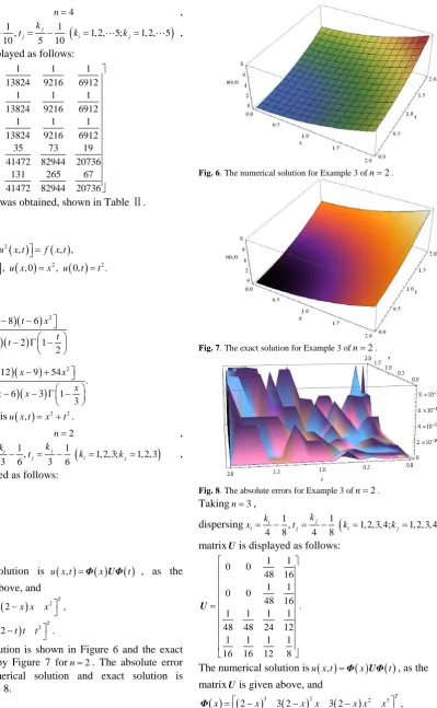
The numerical solution is shown in Figure 6 and the exact solution is given by Figure 7 forn=2. The absolute error between the numerical solution and exact solution is displayed in Figure 8.

Fig. 6. The numerical solution for Example 3 ofn=2.

Fig. 7. The exact solution for Example 3 ofn=2.

Fig. 8. The absolute errors for Example 3 ofn=2_.

Takingn=3,

dispersing 1, 1

(

1, 2,3, 4; 1, 2,3, 4

)

4 8 4 8

j i

i j i j

k k

x = − t = − k = k = , the

1 1 0 0

48 16 1 1 0 0

48 16 . 1 1 1 1 48 48 24 12

1 1 1 1 16 16 12 8

 

 

=  

 

 

U

The numerical solution isu x t

( )

, =Φ

( )

x UΦ

( )

( ) (

)

(

)

(

)

( ) (

)

(

)

(

)

3 2 ₂ ₃

3 2 2 3

2 3 2 3 2 ,

2 3 2 3 2 .

T

x x x x x x x

t t t t t t t

 

=_ − − − _

 

=_ − − − _

Φ

IAENG International Journal of Applied Mathematics, 46:4, IJAM_46_4_05

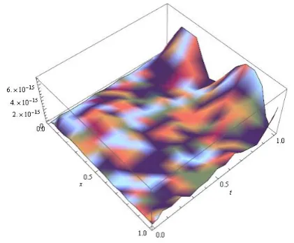
[image:6.595.123.523.46.694.2] [image:6.595.46.286.53.223.2] [image:6.595.42.294.259.627.2]

(7)

The absolute error between the exact solution and the numerical solution is displayed as Figure 9.

Figures1-9 and TablesⅠandⅡ illustrated the absolute error was very small and only a small number of Bernstein polynomials were needed to obtain satisfactory results.

Examples 1-3conveyedthe conclusion that the approach proposed in this paper could be effectively used to identify the numerical solution of the generalised variable order fractional partial differential equation. At the same time, it also proved the feasibility of the method. From the aforementioned examples, numerical solutions were in good agreement with the exact solution. Furthermore, the proposed method was more convenient in computation than the method in [27].

VI. CONCLUSION

This research derived the fractional operational matrix with variable x and t of Bernstein polynomials, which were utilised to identify the numerical solution of generalised fractional partial equations. The operational matrix transformed the initial equation into products of matrices, which could also be viewed as the system of algebraic equations after dispersing the variable. Solving the algebraic equations, the numerical solutions could be obtained.

There are many methods to solve fractional differential equations. The method proposed in this article is simple in theory and easy in computation. Therefore, this method has deserving applications in solving various fractional differential equations.

ACKNOWLEDGMENT

The authors thank the referees for their careful reading of the manuscript and insightful comments, which helped to improve the quality of the paper. We would also like to acknowledge the valuable comments and suggestions from the editors, which vastly contributed to the improvement of the presentation of the paper.

REFERENCES

[1] Leda Galue, S.L. Kalla, B.N. Al-Saqabi, “Fractional extensions of the temperature field problems in oil strata,” Appl. Math. Comput., 186 (2007) 35–44.

[2] Yan Zuomao, Lu Fangxia, “Existence of a new class of impulsive Riemann-Liouville fractional partial neutral functional differential

equations with infinite delay,” IAENG International Journal of Applied Mathematics, vol. 45, no. 4, pp.300-312, 2015.

[3] A. M. A., EI-Sayed, “Nonlinear functional differential equations of arbitrary orders,” Nonliear Analysis, 33(1998) 181-186.

[4] Z. Odibat, “A study on the convergence of variational iteration method,” Mathematical and Computer Modelling, 51(2010) 1181-1192.

[5] Z. Odibat, S.Momani, “Generalized differential transform method: Application to differential equations of fractional order,” Applied Mathematics and Computation, 197(2008) 467-477.

[6] Li, Y. L., Sun, N., “Numerical solution of fractional differential equations using the generalized block pulse operational matrix,”

Computers and Mathematics with Application, 62(2011)1046 -1054. [7] Yi, M. X., Chen, Y. M., “Haar wavelet operational matrix method for

solving fractional partial differential equations,” Computer Modeling in Engineering &Sciences, 88(3) (2012) 229-244.

[8] Asgari M, “Numerical Solution for Solving a System of Fractional Integro-differential Equations”, IAENG International Journal of Applied Mathematics, vol. 45, no. 2, pp.85-91, 2015.

[9] Z. Diethelm, N.J. Ford, “Multi-order fractional differential equations and their numerical solution,” Appl. Math. Comput., 154 (2004) 621–640.

[10] Shang Nina, Zheng Bin, “Exact solutions for three fractional partial differential equations by the (G'/G) method”, IAENG International Journal of Applied Mathematics, vol. 43, no. 3, pp.114-119, 2013. [11] Z. Odibat, S. Momani, “Modified homotopy perturbation method:

application to quadratic Riccati differential equation of fractional order,” Chaos, Solitons & Fractals, 36 (2008) 167–174.

[12] C.F. Lorenzo, T.T. Hartley, Initialization, conceptualization, and application in the generalized fractional calculus, NASA Technical Publication 98–208415, NASA Lewis Reseach Center, 1998. [13] C.F. Lorenzo, T.T. Hartley, “Variable order and distributed order

fractional operators,” Nonlinear Dynamics, 29 (2002) 57–98. [14] C.F.M. Coimbra, “Mechanics with variable-order differential

operators,” Ann. Phys., 12 (11–12) (2003) 692–703.

[15] S.G. Samko, B. Ross, “Intergation and differentiation to a variable fractional order,” Integral Trans. Special Func., 1 (4) (1993) 277–300. [16] S.G. Samko, “Fractional integration and differentiation of variable

order,” Anal. Math., 21 (1995) 213–236.

[17] C.M. Soon, F.M. Coimbra, M.H. Kobayashi, “The variable viscoelasticity oscillator,” Ann. Phys., 14 (6) (2005) 378–389. [18] S.A. Yousefi, M. Behroozifar, Mehdi Dehghan, “The operational

matrices of Bernstein polynomials for solving the parabolic equation subject to specification of the mass,” Journal of Computational and Applied Mathematics, 235 (2011) 5272–5283.

[19] S.A. Yousefi, M. Behroozifar, “Operational matrices of Bernstein polynomials and their applications,” Internat. J. Systems Sci., 41 (6) (2010) 709–716.

[20] S.A. Yousefi, M. Behroozifar, Mehdi Dehghan，“Numerical solution of the nonlinear age-structured population modelsby using the operational matrices of Bernstein polynomials,” Applied Mathematical Modelling, 36 (2012) 945–963.

[21] Chen, Y. M., Yi, M. X., Chen, C., Yu, C. X., “Bernstein polynomials method for fractional convection-diffusion equation with variable coefficients,” Computer Modeling in Engineering & Sciences, 83(6) (2011) 639-653.

[22] E.H. Doha, A.H. Bhrawy, M.A. Saker, “Integrals of Bernstein polynomials: an application for the solution of high even-order differential equations,” Appl. Math. Lett., 24 (2011) 559–565. [23] K. Maleknejad, E.Hashemizadeh, R. Ezzati, “A new approach to the

numerical solution of Volterra integral equations by using Bernsteins approximation,” Communications in Nonlinear Science and Numerical Simulation, 16(2011) 647–55.

[24] BN. Mandal, S. Bhattacharya, “Numerical solution of some classes of integral equations using Bernstein polynomials,” Appl Math Comput., 190(2007) 1707–16.

[25] K. Maleknejad, E. Hashemizadeh, B. Basirat, “Computational method based on Bernstein operational matrices for nonlinear Volterra–Fredholm–Hammerstein integral equations,” Commun. Nonlinear Sci. Numer. Simul., 17 (1) (2012) 52–61.

[26] Mingxu Yi, Jun Huang, Jinxia Wei, “Block pulse operational matrix method for solving fractionalpartial differential equation,” Applied Mathematics and Computation, 221 (2013) 121–131.

[27] Chang-Ming Chen, F.Liu, K. Burrage, “Numerical analysis for a variable-order nonlinear cable equation,” Journal of Computational and Applied Mathematics, 236 (2011) 209–224.

IAENG International Journal of Applied Mathematics, 46:4, IJAM_46_4_05

[image:7.595.63.274.48.222.2]

(8)

TABLE Ⅰ The absolute error of different values of

(

x ti, j

)

whenn=3. i

x t_j t=0.5 t=1.0 t=1.5 t=2.0 t=2.5

0.0

x= 0 0 0 0 0

0.5

x= 7.87476E-14 3.55271E-14 6.68754E-14 3.13163E-14 9.30926E-14 1.0

x= 4.89498E-15 1.77636E-14 4.26485E-14 4.79776E-14 5.94209E-14 1.5

x= 1.66316E-15 7.10543E-14 9.30926E-14 4.93099E-14 1.10862E-14 2.0

x= 8.78271E-15 1.46549E-14 7.73195E-14 4.13163E-14 7.24265E-14 2.5

x= 5.29856E-14 7.99361E-15 6.15463E-14 6.46549E-14 5.50990E-14 3.0

x= 2.76636E-14 5.32907E-15 5.21725E-15 9.10543E-15 3.32747E-15 3.5

x= 9.34527E-14 3.55271E-15 1.77636E-15 5.77636E-15 8.88178E-16 4.0

x= 6.88178E-16 2.13658E-15 3.66454E-15 6.55271E-15 2.44089E-16 TABLE Ⅱ The absolute error of different values of

(

x ti, j

)

whenn=4.

i

x tj t=0.5 t=1.0 t=1.5 t=2.0 t=2.5

0.0

x= 0 0 0 0 0

0.5

x= 2.20476E-15 8.65983E-15 2.26589E-15 5.79315E-16 2.85631E-15 1.0

x= 4.88498E-15 1.02991E-15 2.78526E-15 2.13469E-16 2.24265E-15 1.5

x= 5.42816E-15 1.89621E-15 2.96385E-15 2.13163E-16 3.10862E-15 2.0

x= 3.55271E-15 3.69874E-15 1.27412E-15 2.10574E-15 2.24265E-15 2.5

x= 6.39836E-15 3.74236E-15 1.23654E-15 1.54946E-16 5.62489E-15 3.0

x= 3.56686E-15 5.33669E-15 6.85236E-16 5.54396E-15 6.32697E-15 3.5

x= 1.55747E-15 7.44156E-16 1.75369E-16 2.63677E-15 8.58638E-16 4.0

x= 8.88178E-16 1.66887E-16 9.84265E-16 2.52715E-15 7.32747E-16

IAENG International Journal of Applied Mathematics, 46:4, IJAM_46_4_05

[image:8.595.95.500.68.195.2] [image:8.595.101.503.222.349.2]