Abstract—This paper deals with the estimation of stress strength model R=P(X<Y) when X and Y are two independent inverse Weibull distributions with different parameters. The maximum likelihood estimator and the Bayesian estimate of R are proposed, and the corresponding confidence intervals are obtained. Monte Carlo simulations are performed to compare the different proposed methods.
Index Terms—Maximum likelihood estimator, approximate
confidence interval, bootstrap confidence interval
I. INTRODUCTION
HE problem of making inference about the stress strength model R=P(Y<X) has received a considerable attention. For example, in a reliability study, let X be the strength of a component and Y be the stress applied to the component, then R can be considered as a measure of the component performance. The component fails if and only if at any time the applied stress is greater than its strength. Because R represents a relation between the stress and strength of a component, it is popularly known as the stress-strength model.
Up to now, the stress-strength model R=P(Y<X) has been intensively studied. Various different lifetime distributions are considered to estimate R, such as normal distribution, exponential distribution, Weibull distribution, Burr type X distribution, Laplace distribution, beta distribution, gamma distribution et al. Kotz et al. (2003) collected these choices and presented a review of all methods on a book in the last decades. Mokhlis (2005) studied Burr type III distribution. Saracoglu et al. (2007) studied Gompertz distribution. Kundu et al. (2005, 2006, 2009) studied generalized exponential and three parameter Weibull. Raqab et al. [8-9] studied Burr type X and three parameter generalized exponential. Rezaei et al. (2010) studied generalized Pareto distribution.
In this article, we focus on the estimation of R=P(Y<X), where X and Y follow the two parameters inverse Weibull (IW) distribution. First, the maximum likelihood estimator and its asymptotic distribution are obtained. Based on the asymptotic distribution, the confidence interval of R can also be obtained. Then, the Bayesian estimate and corresponding confidence
Manuscript received October 11, 2016; revised January 13, 2017. This work was supported by the Humanity and Social Science Youth Foundation of Ministry of Education of China (No. 15YJCZH055), the key project of Hubei provincial education department (No.D20172701).
C. P. Li is with the Department of Mathematics, Hubei Engineering University, Hubei, 432000, China. e-mail: [email protected].
H. B. Hao is the corresponding author with the Department of Mathematics, Hubei Engineering University, Hubei, 432000, China. e-mail: [email protected].
interval is obtained. At last, Monte Carlo simulations are performed to compare the different proposed methods.
II. INVERSEWEIBULLDISTRIBUTIONS Due to the convenient structure of its distribution function, the Weibull distribution was used very effectively in analyzing various lifetime data. We know that the hazard function of Weibull is decreasing or increasing depending on the shape parameter. When the data has a non-monotone hazard function, the Weibull distribution cannot be used, and the inverse Weibull (IW) distribution may be an appropriate model (see Kundu D. and Howlader H (2010)).
If a random variable Z has a Weibull distribution with a probability density function (pdf) as
1
( )
exp(
)
f z
=
αλ
z
α−−
λ
z
α ,z
>
0
then, the random variable T=1/Z has an IW distribution with the pdf as
( 1)
( )
exp(
)
f t
=
αλ
t
− +α−
λ
t
−α ,t
>
0
where λ>0 and α>0 are scale and shape parameter respectively. For convenience, we denote the inverse Weibull distribution as IW(α,λ).
In addition, the IW distribution plays some important roles in other areas, such as describing the degradation phenomena of mechanical components, describing the context of a load strength relationship for a component and providing the good fit to survival data. Recently, many authors has been studied this distribution, such as Kundu et al.(2010) Calabria et al.(1994), Murthy et al.(2004), and Gusmao et al. (2009).
III. RELIABILITYMODEL
In this article, we will consider the reliability R when X and Y are independent but not identically IW distributed random variables. Let X be the strength of a component with a stress Y, and suppose X~IW(α,λ1) and Y~IW(α,λ2), respectively,
1
1 1
( )
exp(
)
X
f
x
=
αλ
x
α−−
λ
x
α ,x
>
0
and
1
2 2
( )
exp(
)
Y
f
y
=
αλ
y
α−−
λ
y
α ,z
>
0
where λ1 and λ2 are unknown parameters, and αis a known common parameter.
Therefore, the stress-strength structural reliability model can be expressed as follow
R=P Y( <X) ( 1)
1 1 2
0 x exp[ ( )x ]dx
α α
αλ λ λ
+∞ − + −
=
∫
− +1
1 2
λ λ λ
=
+ (1)
Reliability of a Stress
–
Strength Model with
Inverse Weibull Distribution
Chunping Li, Huibing Hao
T
IAENG International Journal of Applied Mathematics, 47:3, IJAM_47_3_10
From the expression of R, if we get the estimator of the λ1 and λ2, then we can get the estimator of R.
IV. POINTESTIMATIONOFR A. Maximum likelihood estimation of R
To compute the MLE of R, suppose X1, X2,…, Xn is a random sample from IW(α,λ1), and Y1, Y2,…, Ym is a random sample from IW(α,λ2). Based on the observations X and Y, the log-likelihood function will be
1 2 1 1
1 1
( ,
, )
ln
ln
(
1)
ln
n n
i i
i i
L
λ λ α
n
α
n
λ α
x
λ
x
−α= =
=
+
− +
∑
−
∑
∑
∑
= − =−
+
−
+
+
m j j m j jy
y
m
m
1 2 12
(
1
)
ln
ln
ln
α
λ
α
λ
α (2)The MLE’s of λ1 , λ2 and α can be obtained by solve the following equations
0
1 1 1=
−
=
∂
∂
∑
= − n i ix
n
L
αλ
λ
(3)0
1 2 2=
−
=
∂
∂
∑
= − m j jy
m
L
αλ
λ
(4)+
−
−
+
=
∂
∂
∑
∑
= = m j j n i iy
x
m
L
1 1ln
ln
n
α
α
0
ln
ln
1 i 2 1 i1
∑
+
∑
=
= − = − n i j n i
i
x
y
y
x
αλ
αλ
(5)From (3) and (4), we can get 1 1 n ˆ i i
n
ˆ
x
αλ
− ==
∑
(6)and 2 1 m ˆ j j
m
ˆ
y
αλ
− ==
∑
(7)Then αˆ can be obtained as a solution of the non-linear equation as follow
+
−
−
+
=
∑
∑
= = m j j n i iy
x
m
g
1 1ln
ln
n
)
(
α
α
0
ln
ˆ
ln
ˆ
1 i 2 1 i1
∑
+
∑
=
= − = − n i j n i
i
x
y
y
x
αλ
αλ
(8)Here, αˆ can be obtained from the non-linear equation
α
α
)
=
(
h
where1 2
1 1 i 1 i 1
( )
ˆ
ˆ
ln
ln
ln
ln
n m n n
i j i i j i
i j
n m
h
x
y
x
αx
y
αy
α
λ
−λ
−= = = =
+
=
+
−
−
∑
∑
∑
∑
(9)From the non-linear equation (9), we can find that αˆis a fixed point solution and it can be acquired by using a iterative scheme as follow
) 1 ( ) (j
)
(
=
j+h
α
α
(10)whereα( )j is the jth iterate of αˆ.
The iteration procedure should be stopped whenα α( )j − ( 1)j+ is sufficiently small. If we obtainαˆ , thenλˆ1andλˆ2can be obtained from equation (6) and equation (7), the MLE of R can be easily obtained as
2 1 1
ˆ
ˆ
ˆ
ˆ
λ
λ
λ
+
=
R
(11)B. Bayes estimator of R
In this subsection, the Bayes estimation of R under the squared error loss can be obtained. It is assumed that λ1, λ2 and α have independent gamma prior with λ1~GA(a1,b1) and λ2~GA(a2,b2) and α~GA(a3,b3). Based on the above assumptions, we can get the likelihood function as
( 1) ( 1)
1 2 1 2
1 1
(
| ,
,
)
n m
n m n m
i j
i j
l data
α λ λ
α
+λ λ
x
− +αy
− +α= =
=
∏
∏
−
−
×
∑
∑
= − = − m j j n i iy
x
1 2 1 1exp
exp
λ
αλ
αTherefore, we can get the joint density of the data, λ1, λ2 and αas
1 2 1 2 1 2
(
, ,
,
)
(
| ,
,
) ( ) (
) ( )
l date
α λ λ
=
l date
α λ λ π λ π λ π α
where π( )⋅ is the prior distribution.
So the joint posterior density of λ1, λ2 and α given the data is 1 2
1 2
1 2 1 2 0 0 0
(
, , ,
)
( , ,
|
)
(
, , ,
)
l data
l
data
l data
d d d
α λ λ
α λ λ
α λ λ α λ λ
∞ ∞ ∞
=
∫ ∫ ∫
1
(
1,
1 3)
2(
2,
2 4)
GA n a b
λs
GA m a b
λs
∝
+
+ ×
+
+
3 3 1 2
( , ) ( )
GA n m a bα s s Wα
× + + + + × (12)
where
∑
==
n i ix
s
11
ln
,∑
=
=
m j jy
s
12
ln
,∑
= − = n i i x s 1 3
α ,
∑
= − = m j j y s 1 4 α , 1 2
1 3 2 4
( n a ) ( m a ) W(α) ( b= +s )− + ( b +s )− +
Because equation (12) cannot be obtained analytically, therefore, we considered Markov Chain Monte Carlo (MCMC) Method to compute the Bayes estimates. For more details about the MCMC methods, see Upadhyaya et al.[16].
From equation (12), the posterior pdfs of λ1 ,λ2 and α are obtained as follows
(
)
1| 2, ,data~Gamma n a b1, 1 s3
λ λ α + +
(
)
2
|
1, ,
data
~
Gamma m a b
2,
2s
4λ λ α
+
+
and
31 ( 1) ( 1)
1 2 3
1 1
( | , ,
)
exp(
)
n m
n m a
i j
i j
f
αα λ λ
data
α
+ + −b
α
x
− +αy
− +α= =
∝
−
∏
∏
Unfortunately, the posterior pdf α is unknown, but its plots show that it is similar to normal distribution. So the Metropolis–Hastings method can be used.
Therefore, the following MCMC procedure is proposed to compute Bayes estimators of R as follows:
Step 1: Start with initial guess (0) (0) (0)
1 2
(α λ λ, , ), and set t=1.
IAENG International Journal of Applied Mathematics, 47:3, IJAM_47_3_10
Step 2: Using Metropolis–Hastings, generate α(t)
from
f
αwith the
N
(
α
(t−1),
1
)
proposal distribution. Step 3: Generate ( )1 t
λ
from(
)
1, 1 3
G A n+a b + s , and Generate
λ
2( )t from GA m a b(
+ 2, 2+s4)
.Step 4: Compute
R
( )t from equation (11). Step 5: Sett
=
t
+
1
.Step 6: Repeat steps 2–5, Mtimes.
Note that in step 2, we use the Metropolis–Hastings algorithm with
q
~
N
(
α
(t−1),
1
)
proposal distribution as following:a. Let
x
=
α
(t−1).b. Generate
y
from the proposal distributionq
. c. Letp
(
x
,
y
)
=
min{
1
,
[
f
α(
y
)
q
(
x
)]
[
f
α(
x
)
q
(
y
)]
}
. d. Accepty
with probabilityp
(
x
,
y
)
or acceptx
withprobability
1
−
p
(
x
,
y
)
.Now the approximate posterior mean and posterior variance of R become
( )
1
1
ˆ( | ) M t t E R data R
M =
=
∑
,( ) 2
1
1
ˆ( | ) M ( t ˆ( | ))
t
V R data R E R data M =
=
∑
−and
ˆ ˆ
( | ) ( | ) ( | )
MSE R data) =E R data +V R data respectively.
The credible interval of R can be obtained by using numerical integration method. The importance sampling method proposed by Chen et al. (1999) can be used to compute the approximate highest posterior density (HPD) interval. It is not pursued here.
V. INTERVALESTIMATIONOFR A. Approximate confidence interval
In this section, the asymptotic distributions of
θ
ˆ
=
(
λ
ˆ
1,
λ
ˆ
2,
α
ˆ
)
and Rˆ can be obtained. Based on the asymptotic distribution of Rˆ , the asymptotic confidence interval of R can be obtained.
Let us denote the expected Fisher information matrix of
) , , (λ1λ2α
θ= as J(θ)=E(I(θ)), where
I
(
θ
)
=
(
I
ij)
i,j=1,2,3 is the observed information matrix, andI
ij= −∂
2L
∂ ∂
λ λ
i j. It is easy to get that2
11 1
I
=
n
λ
,I
22=
m
λ
22 ,∑
= −
− =
= n
i
i i x x I
I
1 31
13 ln
α ,
∑
= −
−
=
=
mj
j j
y
y
I
I
1 32
23
ln
α ,
0
21 12
=
I
=
I
,2 2 2
33 1 2
1 1
( ) (ln ) (ln )
n m
i i j j
i j
I n m α λ x−α x λ y−α y
= =
= + +
∑
+∑
Theorem 1. As
n
→
∞
,m
→
∞
andp
m
n
→
, then))
,
,
(
,
0
(
)]
ˆ
(
),
ˆ
(
),
ˆ
(
[
1 1 23 2
2 1
1
λ
λ
λ
α
α
λ
λ
α
λ
−
m
−
n
−
→
N
U
−n
where U( ,λ λ α1 2, )=J( )θ is the Fisher information matrix
)) ( ( ) (θ EIθ J = .
Proof: By using the asymptotic normality of MLE and the central limit theorem, the proof is complete.
Theorem 2 As
n
→
∞
andm
→
∞
andp
m
n
→
, then)
,
0
(
)
ˆ
(
R
R
N
B
n
−
→
where
1 1 2
1 2 3 1 2 3
(
R
,
R
,
R
)
( ,
, )(
R
,
R
,
R
)
B
U
λ λ α
λ λ
λ
−λ λ
λ
∂
∂
∂
∂
∂
∂ ′
=
∂
∂
∂
∂
∂
∂
Proof : By using Theorem 1 and Delta method, the proof is complete.
Using Theorem2, we can obtain the asymptotic confidence interval of R is
1 2 1 2
ˆ
ˆ
,
ˆ
ˆ
R
z
−γB n
R
z
−γB n
−
+
It is clear that the asymptotic confidence interval do not perform very well for small sample sizes. So, the bootstrap confidence interval main for small sample sizes is proposed, which might be computationally for large samples.
B. Bootstrap confidence interval
In this section, a percentile bootstrap method (see Efron (1982)) is used to obtain the confidence intervals of R as follows:
Step1: Generate random samples
x x
1, , ,
2L
x
n andy y
1, , ,
2L
y
m from IW(α,λ1) and IW(α,λ2), then compute maximumlikelihood estimators λˆ1,λˆ2 and
α
ˆ
.Step2: Generate a bootstrap sample
x x
1*, , ,
*2L
x
n* from IW(αˆ,λˆ1)and similarly generate a bootstrap sample
y y
1*, , ,
*2L
y
*m from )ˆ , ˆ
IW(α λ2 . Based on these bootstrap samples compute bootstrap estimate of R using equation (11), sayˆ*
R . Step3: Repeat step2 N boots.
Step4: Let H(x)=P(Rˆ*≤x) be the cumulative distribution function of ˆ*
R . Define ˆ ( ) 1( )
x H x RBoot
−
= for a given
x
. The approximate100(1−γ)%bootstrap confidence interval of R is(
ˆ ( 2), ˆ (1 2))
Boot BootR γ R −γ
VI. SIMULATIONRESULTS
In this section, we give some Monte Carlo simulation results to compare the performance of the different methods under the different sample sizes and different parameter values. We mainly compare the performances of the MLE and the Bayes estimates under the squared error loss function in terms of biases, and mean squares errors (MSE). We also compare different confidence intervals, namely the confidence intervals obtained by using asymptotic distributions of the MLE, and the bootstrap confidence intervals in terms of the average confidence lengths, and coverage percentages.
In order to obtain the simulation results, we assume that the sample sizes (n, m) = (5, 5), (10, 10), (15, 15), (20, 20), (25, 25) and (30, 30). From the simulation samples, we compute
IAENG International Journal of Applied Mathematics, 47:3, IJAM_47_3_10
the estimate ofα by using the iterative algorithm equation (10). We have used the initial estimate to be 1(α=1) and the iterative process stops when the difference between the two consecutive iterates are less than 10-6. Once we estimate α, we can get the estimation of λ1 and λ2 by using equation (6) and equation (7). Finally, by using equation (11), we can obtain the MLE of R.
We report the average biases and mean square error (MSE) of Rˆ over 1000 replications. We also report the average biases and MSE of the MLE and Bayes estimators over 1000
replications. The results are reported in Table I and Table II.
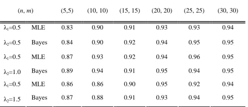
We compute the 95% confidence intervals based on the asymptotic distributions of the MLE. We compute Bootstrap confidence intervals. We also obtain the average confidence credible lengths, and the corresponding coverage percentages. The results are reported in Table IIIand Table IV.
From the above simulation study results, we can get the following conclusions:
(i) Even for small sample sizes, the performance of the MLE and Bayes estimator are quite satisfactory in terms of biases and MSE. Interestingly, the MSE of the MLE are smaller than the MSE of the Bayes estimators in most of the cases. It is observed that when
m
andn
increase, then MSE and biases decrease for all the estimators.(ii) The confidence intervals based on the MLE do not work very well when the sample size is very small, but when
m
andn
greater than 20, the results work quite well. Non-parametric bootstrap methods work quite well, it is observed that bootstrap confidence intervals perform better than the asymptotic confidence intervals, at least for small sizes.(iii) The coverage probability of confidence intervals is slightly below when sample sizes are small.
VII. CONCLUSION
In this paper, we have addressed the problem of estimating R for the inverse Weibull distributions with different shape parameters. Firstly, the maximum likelihood estimator is obtained. Even for small sample sizes, we found that the maximum likelihood estimator works quite well. By using the asymptotic distribution, the asymptotic confidence interval is obtained. It is clear that the asymptotic confidence interval do not perform very well for small sample sizes. So, the bootstrap confidence interval main for small sample sizes is proposed. Based on the simulation results, we recommend using the non-parametric Bootstrap percentile method, when the sample size is very small. Further more, we obtain the Bayes estimate of R under the square error loss function. It is observed that their performances are quite similar, and the performances of the MLE are marginally better than Bayes estimator.
REFERENCES
[1] S. Kotz, Y. Lumelskii and M. Pensky, “The stress strength model and its generalizations: theory and applications”, Singapore: world
scientific. 2003.
[2] N.A. Mokhlis, “Reliability of a stress–strength model with Burr type III distributions,” Commun. Statist. Theor. Meth., vol.34, no.7, pp. 1643-1657, 2005.
[3] B. Saracoglu and M. F. Kaya, “Maximum likelihood estimation and confidence intervals of system reliability for Gompertz distribution
in stress–strength models”, Selcuk J. Appl. Math., no.8, pp.25-36, 2007.
[4] D. Kundu and R.D. Gupta, “Estimation of P(Y<X) for generalized exponential distribution”, Metrika, vol.61, no.3, pp.291-308, 2005. TABLEI
BIAS OF THE MLE AND BAYES ESTIMATION
(n, m) (5,5) (10, 10) (15, 15) (20, 20) (25, 25) (30, 30)
MLE 0.0122 0.0060 0.0013 0.0066 0.0019 0.0006 λ1=0.5
λ2=0.5 Bayes -0.0582 -0.0608 -0.0648 -0.0677 -0.0693 -0.0697
MLE 0.0065 0.0044 0.0046 0.0045 0.0042 -0.0024 λ1=0.5
λ2=1.0 Bayes 0.0110 0.0035 -0.0018 -0.0023 -0.0104 -0.0011
MLE 0.0133 0.0102 0.0072 0.0015 -0.0002 -0.0003 λ1=0.5
λ2=1.5 Bayes -0.0331 -0.0591 -0.0598 -0.0588 -0.0574 -0.0618
TABLEII
MSE OF THE MLE AND BAYES ESTIMATION
(n, m) (5,5) (10, 10) (15, 15) (20, 20) (25, 25) (30, 30)
MLE 0.0267 0.0128 0.0082 0.0059 0.0045 0.0037 λ1=0.5
λ2=0.5 Bayes 0.0414 0.0269 0.0197 0.0158 0.0133 0.0128
MLE 0.0347 0.0151 0.0095 0.0063 0.0053 0.0044 λ1=0.5
λ2=1.0 Bayes 0.0376 0.0223 0.0189 0.0112 0.0081 0.0078
MLE 0.0329 0.0139 0.0084 0.0062 0.0049 0.0041 λ1=0.5
λ2=1.5 Bayes 0.0358 0.0208 0.0161 0.0125 0.0112 0.0103
TABLEIII
AVERAGE CONFIDENCE LENGTHS FOR DIFFERENT ESTIMATION
(n, m) (5,5) (10, 10) (15, 15) (20, 20) (25, 25) (30, 30)
MLE 0.5689 0.3966 0.3263 0.2866 0.2590 0.2308 λ1=0.5
λ2=0.5 Bayes 0.5090 0.3835 0.3190 0.2795 0.2504 0.2295
MLE 0.6234 0.4525 0.3674 0.3171 0.2804 0.2559 λ1=0.5
λ2=1.0 Bayes 0.5538 0.4204 0.3480 0.3040 0.2732 0.2498
MLE 0.5959 0.4225 0.3542 0.3039 0.2748 0.2521 λ1=0.5
[image:4.595.50.298.654.761.2]λ2=1.5 Bayes 0.5369 0.4065 0.3382 0.2952 0.2652 0.2421
TABLE IV
COVERAGE PERCENTAGES FOR DIFFERENT ESTIMATION
(n, m) (5,5) (10, 10) (15, 15) (20, 20) (25, 25) (30, 30)
MLE 0.83 0.90 0.91 0.93 0.93 0.94 λ1=0.5
λ2=0.5 Bayes 0.84 0.90 0.92 0.94 0.95 0.95
MLE 0.87 0.93 0.92 0.94 0.96 0.95 λ1=0.5
λ2=1.0 Bayes 0.89 0.94 0.91 0.95 0.94 0.95
MLE 0.86 0.86 0.90 0.95 0.92 0.94 λ1=0.5
λ2=1.5 Bayes 0.87 0.88 0.91 0.93 0.94 0.95
IAENG International Journal of Applied Mathematics, 47:3, IJAM_47_3_10
[5] D. Kundu and R.D. Gupta, “Estimation of P(Y<X) for Weibull distributions”, IEEE Trans. Reliab, vol.55, pp.270-280, 2006. [6] D. Kundu and M.Z. Raqab, “Estimation of R=P(Y<X) for three
parameter Weibull distribution”, Statist. Probab. Lett, vol.79, pp.1839-1846, 2009.
[7] M.Z. Raqab and D. Kundu, “Comparison of different estimators of P(Y<X)for the Burr Type X distribution”, Commun. Statist. Simul. Computat, vol.34, pp.465-483, 2005.
[8] M.Z. Raqab, M.T. Madi and D. Kundu, “Estimation of P(Y<X) for the 3-parameters generalized exponential distribution”, Commun. Statist. Theor. Meth , vol. 37, pp. 2854-2864, 2008.
[9] S. Rezaei, R.Tahmasbi and M. Mahmoodi, “Estimation of P(Y<X) for the generalized Pareto distribution”, J. Statist. Plan. Infer., vol.140, pp. 480-494, 2010.
[10] D. Kundu and H. Howlader, “Bayesian inference and prediction of the inverse Weibull distribution for Type-II censored data”, Comput Stat Data Anal., vol.54, pp. 1547-1558, 2010.
[11] R. Calabria and G. Pulcini, “Bayesian sample prediction for the inverse Weibull distribution”, Commun. Statist. Theor. Meth., vol.23, pp. 1811-1824, 1994.
[12] D.N.P. Murthy, M. Xie and R. Jiang, “Weibull Models”, New York: Wiley, 2004.
[13] F.R.S. Gusmao, E.M.M. Ortega and G.M. Cordeiro, “The generalized inverse Weibull distribution”, Stat.Pap., vol.50, pp.291-308, 2009. [14] S. K. Upadhyaya, N. Vasishta and A. F. M. Smith, “Bayes inference
in life testing and reliability via Markov chain Monte Carlo
simulation”, Sankhya A, vol.63, pp.15-40, 2001.
[15] M. H. Chen and Q. M. Shao, “Monte Carlo estimation of Bayesian credible and HPD intervals”, J. Computat. Graphic. Statist. vol.8, pp.69-92, 1999.
[16] B. Efron, “The jackknife, the bootstrap and other re-sampling plans”, Philadelphia, PA: SIAM, CBMS-NSF Regional Conference Series in
Applied Mathematics. vol. 38, 1982.
[17] J. Lai, L. Zhang, C.F. Duffield and L. Aye, “Engineering reliability analysis in risk management framework: development and application
in infrastructure project”, IAENG International Journal of Applied Mathematics, vol.43, no.4, pp. 242-249, 2013.
[18] H. Assareh and K. Mengersen, “Bayesian estimation of the time of a decrease in risk-adjusted survival time control charts”, IAENG International Journal of Applied Mathematics, vol.41, no.4, pp.
360-366, 2011.