Multiple Parameter Based Clustering (MPC): Prospective Analysis for Effective Clustering in Wireless Sensor Network (WSN) Using K Means Algorithm

Multiple Parameter Based Clustering (MPC): Prospective

Analysis for Effective Clustering in Wireless Sensor

Network (WSN) Using K-Means Algorithm

Asif Khan, Israfil Tamim, Emdad Ahmed, Muhammad Abdul Awal Department of EECS , North South University, Dhaka, Bangladesh

Email: alaxwest@yahoo.com, israfiltamim@hotmail.com, {emdad, abdulawal}@northsouth.edu

Received October 15, 2011; revised November 24, 2011; accepted December 21,2011

ABSTRACT

In wireless sensor network cluster architecture is useful because of its inherent suitability for data fusion. In this paper we represent a new approach called Multiple Parameter based Clustering (MPC) embedded with the traditional k-means algorithm which takes different parameters (Node energy level, Euclidian distance from the base station, RSSI, Latency of data to reach base station) into consideration to form clusters. Then the effectiveness of the clusters is evaluated based on the uniformity of the node distribution, Node range per cluster, Intra and Inter cluster distance and required energy level of each centroid. Our result shows that by varying multiple parameters we can create clusters with more uniformly distributed nodes, minimize intra and maximize inter cluster distance and elect less power consuming cen-troid.

Keywords: K-Means Algorithm; Energy Efficient; Uniform Distribution; RSSI; Latency

1. Introduction

Wireless sensor networks (WSN) are highly distributed networks of autonomous small, lightweight sensors (nodes) in large numbers to monitor physical or environmental conditions by the measurement of, temperature, sound, vibration, pressure, motion or pollutants and to coopera- tively pass their data through the network to a main loca- tion (often called a sink).

It has already made its way in military object, habitat monitoring [1] and object tracking because of the char-acteristics such as feasibility of rapid deployment, self- organization (different from Infrastructure Mode or ad hoc network [2]) and fault tolerance. But limited compu- tation capability, limited power and small memory size has made designing the WSNs is very difficult [3]. The energy consumption is the most important factor among these three factors, because the battery is not changeable if once the sensor nodes are deployed. The energy is also the major consideration in designing the routing of the WSNs. Hierarchical protocols reduce energy consump- tion in the networks by clustering. Clustering algorithms partition data objects (patterns, entities, instances, obser- vances, units) into a certain number of clusters (groups, subsets, or categories).

Several available operational definitions [4] summa- rized by Everitt (1980) are as follows:

“A cluster is a set of entities which are alike, and enti-ties from different clusters are not alike.”

A cluster is “an aggregate of points in the test space such that the distance between any two points in the cluster is less than the distance between any point in the cluster and any point not in it.”

“Clusters may be described as continuous regions of this space (d-dimensional feature space) containing a rel- atively high density of points, separated from other such regions by regions containing a relatively low density of points.”

In these protocols, nodes are divided into some clus-ters and some nodes based on some parameter are the selected as cluster heads (CH). These cluster heads ex-change data with the Base station (BS) which costs the most energy of the nodes. Even though this concept has similarity with the Basic Service set (BSS) of Infrastruc-ture mode where there is an Access point (AP) [5] (here the CH) and few cells communicate via this access point, the method in WSN is much more dynamic and energy efficient. Due to these advantages, sensor nodes can re- markably save their own energy.

In this paper by we have proposed a new method called MPC (Multiple Parameter based Clustering) using k-means clustering algorithm and variation of parameter and thus made four contributions:

distribu-tion by considering various parameter combinadistribu-tions. Thus we can avoid clusters with poor distribution of node or highly dense clusters. The base station can centrally de- sign the network with Good clusters by our given criteria.

2) A good cluster can be defined in a new way with the following property:

a. Node distribution is approximate uniform b. Inter-cluster distance is high

c. The intra-cluster distance is low and thus

d. The ratio of intra and inter cluster distance called validity is low

3) Minimum and maximum range of nodes in each cluster varies with parameters.

4) By adding valid parameter we can choose low en-ergy consuming centroid and thus make a low enen-ergy consumed network.

The remainder of the paper is organized as follows. In the following section, related work is discussed. We, then briefly describe k-means algorithm in Section 3. Imple- mentation of scheme is described in Section 5 followed by the experimental results in Section 6. Section 7 pre- sent our conclusion and direction for future works.

2. Related Work

For clustering various parameters have been taken into consideration. The most popular clustering mechanism LEACH [6,7] along with LEACH-C has taken residual energy level of the nodes for cluster head selection for creating clusters. It has been achieved by setting the probability of a node, becoming a cluster-head as a function of nodes energy level relative to the aggre- gate energy remaining in the network rather than purely as a function of the number of times the node has been cluster-head:

 

i

P t

 

 

_{ }

total

E t

P t k

E t



Where Ei(t) is the current energy of node i, and

 

 

1

N

total i

i

E t E t





_

The main drawback of LEACH is that the number of cluster heads is uncertain and there is a chance of poor clustering while LEACH-C requires the position of the entire sensors to avoid this problem. On the Other hand instead of considering node energy level ACE [8] has considered node degree for clustering by using an expo-nentially decreasing function for fmin:

1

min 2

t k

cI f _e k _

 d

In this formula, t is the time passed since the protocol began and cI is the duration of the protocol as described earlier. d is the estimated average degree (number of

neighbors) of a node in the network, and is pre-calculated prior to deployment. k1 and k2 are chosen constants that determine the shape of the exponential graph.

Clustering using Genetic Algorithm [9] distance be- tween nodes and number of cluster heads has been taken into account While Gupta [10] in their method selected residual energy of the nodes, the number of neighbor nodes and centrality for clustering.

Scott Fazackerley [11] proposed a cluster head selec- tion algorithm that uses RF signal strength for head se- lection which is widely implemented in many commer- cial radios. A cluster head is selected based on its per- ceived RF signal strength of its neighbors. This approach has several advantages. First, unlike relying on Euclidean distance which requires localization or network knowl- edge, using RF signal strength compensates for the net- work properties. Nodes closed by distance may not be closed by signal requiring more power for transmissions. This also compensates for dead spots, uneven propaga- tion, and changing RF propagation characteristics. Addi- tionally, cluster heads located in areas of higher node density are expected to have a lower average distance between end nodes and the cluster head. So, it is clear that various parameters are chosen for different cluster- ing algorithm.

Based on above studies we wanted to investigate the effect of taking all these parameters into consideration together while clustering.

3. A Brief Description of K-Means

Algorithm

K-Means clustering is an algorithm to classify or to group given objects based on attributes or parameters, into K number of groups. K is a positive integer number. The K-Means clustering algorithm was developed by J. Mac- Queen (1967) and then by J. A. Hartigan and M. A. Wong around 1975. The grouping is done by minimizing the sum of squares of distances between data and the corre- sponding cluster centroid

Given k, the k-means algorithm is implemented [12] in 4 steps:

1. Partition objects into k nonempty subsets and Com-pute seed points as the centroids z1 (1), z2 (1), z3 (1),….,zK (1) of the clusters of the current partition.

2. At the k-th iterative step, distribute the object {x} among the K clusters using the relation,

 

 

 

j j i

x C k if x z k   x z k

For all i = 1,2,…., K; i ≠ j; where Cj(k) denotes the set of samples whose centre is zj(k).

3. Compute the new cluster centers zj(k+1), j =1, 2, …,

The measure which minimizes this is simply the sample mean of Cj(k). Therefore, the new cluster centre is given

by





 

1 1

j k

j

x C j

Z k x

N 

 

_

where j= 1,2,3...K and Njis the number of samples in Cj(k). 4. Go back to Step 2, stop if zj(k+1) = zj(k) for j = 1, 2, …, K then the algorithm has converged and the pro-cedure is terminated. Otherwise go to Step 2.

4. Parameters

Selecting appropriate parameter for any given WSN is another challenge. But here we wanted to put forward those parameters which are common for almost all WSN. For that most of the parameters we have chosen are re-lated to basic hardware level. They are [13] residual en-ergy level of the nodes, Transmission range (often char-acterized by RSSI), Modulation type, Distance (among the nodes, from the BS etc), Node density, Node angel, Centrality, bit rate, Turn on & wake up time, Processing power, Latency. We have selected Nodes energy. Dis-tance from the BS, RSSI and Latency for our experiment which we think cover most of the real life scenarios and application.

4.1. Nodes Energy

W. heinzelmann et al. [3,4] used node energy level 2J where other research has used range varying from 1J to 5 J [14] In our experiment the energy of node is varied between 1J to 3J.

4.2. Distance

One of the most significant factors for WSN is distance. The position of the base station in the wireless sensor network has great impact on the transmission and the receiving signal strength.

For our experiment we have considered the Euclidian distance from the base station (BS) to each node. It var-ied from 85 m to 175 m. The higher the distance more energy is required to data interchange

Euclidian distance =



 



4.3. Received Signal Strength Indication (RSSI)

The relationship between RSSI (Received Signal Streng- th Indication) values and distance is the foundation and the key of ranging and positioning technologies in wire- less sensor networks [15].

As the use of RSSI ranging need less communication overhead, lower implementation complexity, and lower cost, so it is very suitable for the nodes in wireless sensor network which have limited power.

The principle of RSSI ranging describes the

relation-ship between transmitted power and received power of wireless signals and the distance among nodes. This rela-tionship is:

 

P P (1) Where Pr is the received power of wireless signals, Pt is the transmitted power of wireless signal, d is the dis-tance between the sending nodes and n is the transmis-sion factor whose value depends on the propagation en-vironment.

Take 10 times the logarithm of both sides on (1) then Equation (1) is transformed to Equation (2).

10 lg 10 lg 10 P_r P_t n log d (2)

Pr, the transmitted power of nodes, is given 10 log P is the expression of the power converted to dBm. Equation (2) can be directly written as Equation (3).





R

P Bm  A n g d (3)

By Equation (3), we can see that the values of pa-rameter A and papa-rameter n determine the relationship between the strength of received signals and the distance of signal transmission.

For our experiment we have taken the RSSI value from 0 to 100 dB converting the dbm value collected by the nodes by the BS [14].

RSSI (dB) = 10 log t

r

P P

4.4. Latency

Clustering in WSN should take into account the latency [16]. Latency is an important factor for system reliability such as the case of emergency response, and accuracy of data reporting in case of high frequency periodical data updates. On the other hand, energy consumption is essen- tial to ensure survivability of sensor nodes and hence the lifetime of the system. In a Multihop network, significant delay occurs at each hop due to contention for the wireless channel, packets processing and queuing delay. The latency is therefore a function of the number of communication hops between the source and the gateway (CH). Latency is also a dependent on distance. For our experiment our net-works latency is a function of distance. As the distance increases the latency increases and vice versa.

5. Implementation of Scheme

Assumptions:

1) All nodes have same and adequate amount initial energy.

2) Each node or sink has ability to transmit message to any other node and sink directly.

4) Each sensor node has location information and fixed after deployment.

Then the effectiveness of the clusters is evaluated based on the uniformity of the node distribution, Node range per cluster, Intra and Inter cluster distance and re-quired energy level of each centroid.

5.1. Average Node Distribution

Assume that there are N nodes distributed uniformly in an M × M region. If there are k clusters there are on average N/k nodes per cluster (one cluster head and (N/k)—1 non cluster head nodes). As we have tested with 21 nodes,

Table 1 shows the required nodes per cluster below.

5.2. Intra-Cluster Distance

This is the distance between a point and its cluster centre [9] to determine whether the clusters are compact. We take the average of all of these distances, defined as

2

1

1 K

i i x Ci

intra x z

N  





where N is the number of nodes in the network, K is the number of clusters, and zi is the cluster centre of cluster Ci.

We obviously want to minimize this measure.

5.3. Inter-Cluster Distance

This is the distance between clusters [9]. We calculate this as the distance between cluster centers, and take the minimum of this value, defined as





;

i j

intermin z z

i = 1, 2,…., K–1 and j = i+1, ….., K

we take only the minimum of this value as we want the smallest of this distance to be maximized, and the other larger values will automatically be bigger than this value.

5.4. Distribution Policies:

For the use in simulation the generated random numbers must be transformed to random variables using suitable distribution method.

Uniform Process Generator:

Let X be a uniformly distributed random variable with probability density function

 

f x b a 

 , a < x < b

 

y x a

f X

b a b a



 

 



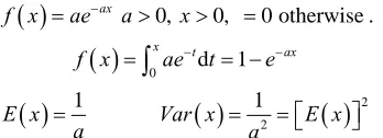
and X = a + (b–a) r Is the required process generator Exponential Process Generator:

 

f x _ae a_ x_{ }

.

 

f x _ ae t_{ }e



 

E x a

 Var x

 

 

a

  _ _

By inverse technique, R = 1–e–ax or 1–R = 1–e–ax X = –(1/α) ln R, since R is likely to occur as 1–R = –E(x). ln R where R is IID (Independent Identically Distributed). For our experiment we have chosen Uniform Process Generator but future work can investigate more with negative Exponential Process Generator.

6. Experimental Results

In our work we carry out our simulation with 21 sensors deployed randomly assuming that they are deployed in clusters with inter-clusters communication will happen only through cluster heads of the respective clusters. Ta-ble 2 shows the simulation parameters.

6.1. Uniform Distribution

When we compare the effect of multiple parameters in two clustered network, we see that (Figure 1) about 83% of the clusters based on the various combinations of two pa- rameters are uniformly distributed to the theoretical value while 50% of clusters are uniform for one parameter.

When we observe the node distribution in the three clustered network, we find that a combination of two pa- rameters (Node energy level & Euclidian distance from BS) results 100% uniform node distribution in each clus- ter which reveals a significant intersection point of three lines on the theoretical value base line (Figure 2).

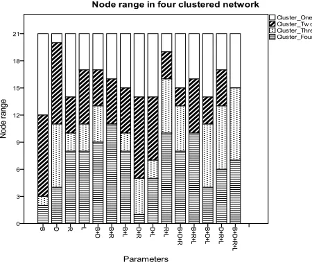
6.2. Maximum and Minimum Range of Node

We see in the four clustered network that change in the parameter combination results in an alternation in the range (maximum to minimum) of nodes per cluster. Our experiments show that (Figure 3) by increasing or de-creasing we can alter node range in any specific cluster.

Table 1. Average nodes per cluster for our experiment.

Number of clusters Average nodes/cluster

2 10.5 3 7 4 5.3 5 4.2

Table 2. Parameters used in simulation study.

Parameter Value

Node energy (B) 1J - 3J

Distance from the Base Station (D) 85 m - 175 m

RSSI (R) 0 to 100 dBm

Latency (L) Depends on the distance

Figure 1. Comparison of node distribution in two clustered network based on multiple parameter.

Figure 2. Achieving uniform node distribution in three clustered network based on multiple parameter.

6.3. Intra Cluster Distance

One of the significant observations of our experiment is that the goal of minimizing the intra cluster distance can be achieved by choosing the right combination of the pa-rameters. For example, in two clustered network combina-tion of three parameters results in minimum intra cluster distance (0.253125 m) while for five clustered network two parameters results the least (0.350227 m). Table 3

represents the results we got from the experiments below:

6.4. Inter Cluster Distance

We can see that minimizing the inter cluster distance results maximization in the intra cluster distance (Figure 4). High Inter cluster distance reduces the cross talk or interference and high power consumption [17].

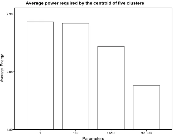
6.5. Centroids with Low Power Requirement

If the clusters that we choose have centroids with high energy that will results in a less energy efficient. From our experiment we see that the increase in the number of pa- rameter in five clustered network (Figure 5) results in centroids with low power requirement for the same cluster.

Table 3. List of intra cluster distance for multiple parame-ters for different cluster size.

Cluster

size Parameter 1

Parameter 1 + 2

Parameter 1 + 2 + 3

Parameter 1 + 2 + 3 + 4

2 0.599375 0.363571 0.253125 0.3375

3 0.356653 0.40558 0.463931 0.466716

4 1.322795 0.358161 0.735257 0.344215

5 0.504306 0.350227 0.746725 0.437796

Figure 4. Relationship between intra and inter cluster distance.

7. Conclusions and Future Works

7.1. Parameter Combination

For our experiment we have chosen 4 parameters which leads to a variation of 24 = 16. Now if the number of pa-rameters increases the number of combination will in-crease exponentially, which will eventually lead to NP complete problem. Various techniques can be applied to solve this kind of problems. For instance In LEACH-C [6] the BS finds clusters using the simulated annealing algo-rithm to solve the NP-hard problem of finding k optimal clusters.

7.2. Which Parameter to Choose?

Different WSN is made up for different purposes. So the effect of parameters will vary from network to network. In out experiment we tried to work with those parameters which are common for almost all the sensors. But finding the right combination of parameters and their optimum value for specific WSN is a great challenge.

7.3. Data Type

For our experiment we have worked with uniform dis-tributed data type. Further experiment can be done by choosing exponential, Negative exponential distribution.

7.4. Platform

We have used python for our experiment because of its robustness and efficiency to deal with huge number of data. But while conducting this experiment we were not aware of any tools that can perform the same functional-ity. Experiments our concept using different program-ming language and compare our data with the output can pave the way to further research field.

REFERENCES

[1] A. Cerpa, et al., “Habitat Monitoring: Application Driver for Wireless Communications Technology,” Science, Vol. 31, No. 2, 2001, pp. 20-41.

[2] K. S. Arefin and E. Ahmed, “Cross-Layer Design of Wireless Networking for Parallel Loading of Access Points (PLAP),” 10th International Conference on Com- puter and Information Technology, 2007, pp. 1-5. doi:10.1109/ICCITECHN.2007.4579444

[3] M. A. Mehr, “Design and Implementation a New Energy Efficient Clustering Algorithm Using Genetic Algorithm for Wireless Sensor Networks,” Engineering and Tech- nology, Vol. 53, No. 2, 2011, pp. 430-433.

[4] R. Xu, I. Donald and C. Wunsch, “Clustering,” IEEE Press, New Jersey, 2009.

[5] K. S. Arefin, E. Ahmed and Z. Alom, “Cross-Layer De- sign of Wireless Networking for Parallel Loading of Ac- cess Points and Mirrored Servers (APMS ),” Access, pp. 2-5.

[6] W. B. Heinzelman, P. Chandrakasan and H. Balakrishnan, “An Application-Specific Protocol Architecture for Wireless Microsensor Networks,” IEEE Transactions on Wireless Communications, Vol. 1, No. 4, 2002, pp. 660- 670.doi:10.1109/TWC.2002.804190

[7] W. Heinzelman and A. Chandrakasan, “Energy-Efficient Communication Protocol for Wireless Microsensor Net- works,” Proceedings of the 33rd Hawaii International Conference on System Sciences, 2002, pp. 1-10.

[8] H. Chan and A. Perrig, “ACE: An Emergent Algorithm for Highly Uniform Cluster Formation,” Wireless Sensor Networks, Vol. 2920, 2004, pp. 55-67.

doi:10.1007/978-3-540-24606-0_11

[9] S. Jin, M. Zhou and A. S. Wu, “Sensor Network Optimi- zation Using a Genetic Algorithm,” Direct, Vol. 4, No. 0, 2001, pp. 1-6.

[10] I. Gupta, D. Riordan and S. Sampalli, “Cluster-Head Election Using Fuzzy Logic for Wireless Sensor Net- works,” 3rd Annual Communication Networks and Ser- vices Research Conference (CNSR’05), Halifax, 2005, pp. 255-260.

[11] S. Fazackerley, P. Alan and R. Lawrence, “Cluster Head Selection Using RF Signal Strength,” Discovery, Univer- sity of British Columbia, Okanagan, 2011.

[12] S. Ray and R. H. Turi, “Determination of Number of Clusters in K-Means Clustering and Application in Col- our Image Segmentation,” Image, In: N. R. Pal, A. K. De and J. Das, Eds., Proceedings of the 4th International Conference on Advances in Pattern Recognition and Dig-ital Techniques, Calcutta, 27-29 December, 1999. [13] J. L. Hill, “System Architecture for Wireless Sensor

Networks by,” PhD Thesis, 2003.

[14] A. Depedri, A. Zanella and R. Verdone, “An Energy Effi- cient Protocol for Wireless Sensor Networks,” Energy, Vol. 134, 2011, pp. 1-6.

[15] J. Xu, “Distance Measurement Model Based on RSSI in WSN,” Wireless Sensor Network, Vol. 2, No. 8, 2010, pp. 606-611.doi:10.4236/wsn.2010.28072

[16] B. Aoun and R. Boutaba, “Clustering in WSN with La- tency and Energy Consumption Constraints,” Journal of Network and Systems Management, Vol. 14, No. 3, 2006, pp. 415-439.doi:10.1007/s10922-006-9039-4