Approximate dynamic programming algorithms for multidimensional flexible production inventory problems

(1)

Approximate dynamic programming algorithms for

multidimensional flexible production-inventory problems

∗

Mustafa C

¸ imen

a†

and Chris Kirkbride

b

a_{Hacettepe University Business Administration Department, 06800 Beytepe, Ankara, Turkey}

b_{Department of Management Science, Lancaster University Management School, Lancaster,}

LA1 4YX, UK

Abstract

An important issue in the manufacturing and supply chain literature concerns the optimization of inventory decisions. Single-product inventory problems are widely stud-ied and have been optimally solved under a variety of assumptions and settings. How-ever, as systems become more complex, inventory decisions become more complicated for which the methods/approaches for optimizing single inventory systems are inca-pable of deriving optimal policies. Manufacturing process flexibility provides an exam-ple of such a comexam-plex application area. Decisions involving the interrelated product inventories and production facilities form a highly multidimensional, non-decomposable system for which optimal policies cannot be readily obtained. We propose the method-ology of Approximate Dynamic Programming (ADP) to overcome the computational challenge imposed by this multidimensionality. Incorporating asample backup simula-tion approach, ADP develops policies by utilizing only a fracsimula-tion of the computasimula-tions required by classical Dynamic Programming. However, there are few studies in the lit-erature that optimize production decisions in a stochastic, multi-factory, multi-product inventory system of this complexity. This paper aims to explore the feasibility and rel-evancy of ADP algorithms for this application. We present the results from numerical experiments that establish the strong performance of policies developed via temporal difference ADP algorithms in comparison to optimal policies and to policies derived from a deterministic approximation of the problem.

Keywords: approximate dynamic programming; machine learning, dynamic program-ming, flexible manufacturing; process flexibility; inventory control

1 Introduction

Manufacturing flexibility is a widely used practice to cope with environmental uncertainty. Technological developments and evolving market requirements over time have resulted in a long history of research in flexibility that is broad and varied (see, for example, Gustavsson (1984); Sethi and Sethi (1990)). Many manufacturing flexibility applications have been

(2)

[image:2.612.74.509.48.194.2]

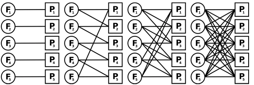
Figure 1: Example system designs for a 5-product, 5-factory system. From left to right: dedicated design, 2-chain design, 3-chain design and full flexibility design.

studied including routing inventory, training labour, contracting, pricing and machinery. For a recent review see Jain et al. (2013). The focus of this paper is process flexibility. This can be categorized as a type of machine flexibility with the ability to produce more than one product in a single factory. Best practice, in terms of production capacity utilization, is having full flexibility where each factory can produce all products. However, full flexibility requires a large degree of investment that includes machinery, training, spare parts, raw materials, etc. Early studies focussed on having either a dedicated system (no flexibility) or full flexibility. A key development by Jordan and Graves (1995) showed that a fraction of this investment, through limited flexibility, could be almost as beneficial as full flexibility when the system is designed appropriately. They suggest a chaining design, which links every product and factory with each other by forming a chain of production abilities across the system (Figure 1). Hence, production can be moved along the chain to match excess demand with unutilised capacity. Limited flexibility via 2- or 3-chain designs are shown to provide the majority of the benefits of full flexibility in terms of demand coverage.

The study of Jordan and Graves increased the interest in this field from both the aca-demic and practical point of view and a significant literature on the benefits and outcomes of limited process flexibility has emerged since 1995. See Chou et al. (2008) for a review of the process flexibility literature. More recently see, for example, Francas et al. (2009); He et al. (2012); Tanrisever et al. (2012); Deng and Shen (2013); Simchi-Levi and Wei (2015); Rafiei et al. (2016); Soysal (2016a). Despite the interest in limited process flexibility, little attention is given to the challenge of optimizing production decisions over time in such sys-tems. Although providing the ability to handle demand variation more efficiently, process flexibility substantially complicates production decisions made in response to inventory levels and ongoing demands. The indirect and direct linkage of all factories and products requires production decisions to be made with respect to the overall production of the system. The interrelated nature of inventory levels to production decisions results in a complex, non-decomposable decision problem, which cannot be solved by classical Dynamic Programming (DP) methods due to the associated computational limitations. A proposition is Approxi-mate Dynamic Programming (ADP) algorithms for optimizing production decisions in this complex production-inventory problem (see Sutton and Barto (1998); Powell (2007)).

(3)

of only a fraction of states based on past events in the simulation. ADP methods have been applied to various inventory problems and settings. Van Roy et al. (1997) introduced an “online temporal-difference method” with approximated policy values, to optimize a two-echelon inventory system. Topaloglu and Kunnumkal (2006) studied a single-product, multi-location inventory system with multiple production plants. Kunnumkal and Topaloglu (2008) introduced ADP methods to find optimal base-stock levels for newsvendor problems and also an inventory purchasing problem assuming that price is unknown, and concluded that using these methods guarantee that iterations will converge to the optimal solution. Wu et al. (2016) consider a multi-product, multi-machine two-stage production system with value function estimation via Artificial Neural Networks (ANN).

The aim of this paper is to investigate the feasibility of ADP algorithms in developing effective policies for optimizing production decisions in process flexibility systems. This requires the tuning of the parameter settings required for ADP algorithms in this complex inventory optimization problem. To this end, we will consider tractable inventory problems which are small enough to be solved by DP value iteration, yet are rich enough to retain the flexibility challenges of large-scale problems. The paper is organized as follows. In Section 2, we describe the process flexibility inventory problem. In Section 3, the ADP approaches utilised are introduced and the parameter settings of the ADP algorithms are explained. Section 4 presents the results of the numerical experiments conducted under different ADP parameter settings and compares the performance of these derived policies to the performance of an optimal policy. The ADP algorithm performance is additionally compared to that of a policy derived from a deterministic approximation of the problem. Finally, in Section 5, a conclusion of the study is provided and directions for future research are outlined.

2 A production-inventory control problem with

pro-cess flexibility

We focus upon a single-echelon, periodic review, capacitated stochastic inventory problem under assumed process flexibility operations. This problem design corresponds to continuous production systems in which multiple products may be produced at each of the available fa-cilities. Given that we shall establish process flexibility operations in a continuous production environment, set-up costs and lead times are assumed to be negligible. A frequently cited example of such systems arises in the automotive industry. However, this can be adapted to other industries which utilise process flexibility in their production systems such as the textile industry, the semiconductor/electronics industry or in service industries such as call centres. See, for example, Chou et al. (2010).

The production-inventory system comprises P products andF factories. Inventory stor-age and factory production capacities limit the amount of products stocked in each warehouse and produced at each factory respectively. Each factory is assumed to have a total produc-tion capacity, Cf, 1 ≤ f ≤ F, and the inventory capacities of each product is given by Ip, 1≤p≤P. The ability of factoryf to produce product p is described as a link between f and p; and is defined as lf,p = 1 (conversely, lf,p = 0 implies no production capability).

The set of states for product p is Ωp = {0, . . . , Ip} with the set of system states given by

I =XP

p=1Ωp.

(4)

each product across all factories. The state of the system at the beginning of a period is denoted i ∈ I where i = (i1, i2, ..., iP) and ip ∈ Ωp is the inventory level of product p. In

state i, the set of feasible actions, A, comprises all allowable factory production capacity allocation combinations. Each element of set A is given by

a= ( qf,p; P X p=1 qf,p Cf

≤1; 1 ≤f ≤F; 1≤p≤P

)

where qf,p are the units of total production capacity allocated to product p at factory f.

Clearly, qf,p = 0 when lf,p= 0.

Production is make to stock and stochastic demand, Dp, for product p is assumed to

be Poisson with mean ηp each period. Any stock held at the end of a period generates

holding cost hp per item. In a stock-out situation, excess demand will be lost with penalty cost θp per item. The unit factory production cost of a product is denoted uf,p. We ignore

production lead times and assume that holding inventory does not induce holding costs until the end of the period which are common assumptions in inventory literature (e.g., Tarim and Kingsman, 2004; Soysal, 2016b). Under action a in inventory state i the expected (one-period) production-inventory costs are given by

Ra_i =

P X p=1 F X f=1

uf,pqf,p

+

P X

p=1

ip+PFf=1qf,p

X

dp=0

P(Dp =dp)

(

hp ip+

F X

f=1

qf,p−dp

!) + P X p=1 ∞ X

dp=ip+PFf=1qf,p

P(Dp =dp)

(

θp dp−ip−

F X f=1 qf,p !) . (1)

The three terms on the r.h.s. of (1) represent the production costs under action a, the expected holding costs paid for any outstanding stock held at the end of the period and the expected penalty costs paid for any unmet demand, respectively.

The optimization objective is to determine a stationary policy π ∈ Π governing the actions taken that minimizes the expected long-run discounted inventory costs over an infinite horizon,

min

π∈ΠE

π

( _∞

X

t=0

γtRa_i )

,

whereγis a discount rate. This optimization problem presents a considerable challenge. The non-decomposable nature of the system means that state and action spaces are highly mul-tidimensional. For a system withP products, with each product having I units of inventory capacity, the state space comprises (I + 1)P _{states. The action space grows exponentially}

with the number of links. In a X-flexibility design there are

F Y

f=1

Cf +X

X !

(5)

so-called curse of dimensionality renders classical DP infeasible. This motives a requirement for the development of approaches that can produce strongly performing heuristics for the problem.

3 Approximate dynamic programming algorithms

DP and ADP algorithms utilise thevalue function(orcost-to-gofunction),V(i), representing the minimum expected long-run discounted costs for a system starting in statei. In classical DP value iteration, value function estimates are stored in a so-calledlook-up table for use in the DP recursion

V(i) = min

a∈A (

Ra_i +γX

i0

β_i,ia0V(i0)

)

, (2)

where Ra

i is the expected one-period cost defined in (1) andβi,ia0 =QP_p₌₁β_ia

p,i0p is a transition

probability from state i to successor state i0 under action a, where

β_ia_p_,i0

p =                                    P∞

dp=ip+PFf=1qf,pP(Dp =dp), i

0

p = 0,

P(Dp =ip+PF_f₌₁qf,p−i0p), 0< i

0

p < Ip ≤ip+PF_f₌₁qf,p,

Pip+PFf=1qf,p−Ip

dp=0 P(Dp =dp), i

0

p =Ip ≤ip+

PF

f=1qf,p,

P(Dp =ip+

PF

f=1qf,p−i0p), 0< i0p ≤ip+

PF

f=1qf,p< Ip,

0, otherwise.

A classical DP value iteration algorithm requires the enumeration of the entire state space, a minimisation over all feasible actions for each state and, for each action, an expectation is calculated. This process, called full backup, continues iteratively until the value functions converge which, for the problem described in Section 2, becomes computationally burden-some for even small problems.

Look-up table ADP algorithms use the same storage of value function estimates and the functions are updated iteratively. However, rather than a full backup viabackward iteration, ADP uses a sample backup approach with forward iteration. Starting from an initial state (or states), a typical ADP approach is to simulate the system and observe realizations of the random outcomes. The simulated information is used to learn about and improve estimates of the value functions, here denoted ˆV(i). The benefit of ADP algorithms in this setting is to be able to develop strongly performing heuristic production policies with significant reductions in the computation time over classical DP.

(6)

Algorithm 1 ADP Pseudo-algorithm

1: STEP 1: Initialization

2: Initialize value functions ˆV(i) ∀i∈ I

3: Choose an initial state i∈ I

4:

5: for (each iteration of the simulation) do

6: STEP 2: Action Selection

7: Choose action ˆa∈A

8:

9: STEP 3: Observe System Feedback

10: Observe exogenous information dp ∀ p∈P

11: Observe successor state i0 ∈ I and immediate return ˆr

12:

13: STEP 4: Value Function Update and Learning

14: Update ˆV(i) by

15: Vˆ(i)←αrˆ+γVˆ(i0)+ (1−α) ˆV(i)

16:

17: STEP 5: Move to Next Iteration

18: i←i0

19:

20: end for

selecting an action greedily by substituting the current estimates of the value functions ˆV(i) in (2) and taking the minimising action; or selecting the action randomly using a probability function over the action space A in state i that accords a higher selection probability to actions promising lower expected future costs. In Step 3 we observe the results of taking action ˆa in state i. As a result of the exogenous information, a sample realisation of the stochastic demand for products, dp, and action ˆa the system will evolve to a new inventory

state i0 and a return

ˆ

r=

P X

p=1

F X

f=1

uf,pqf,p+

P X

p=1

hp ip+

F X

f=1

qf,p−dp

!+

+

P X

p=1

θp dp−ip−

F X

f=1

qf,p

!+

(3)

from the system is generated. Where in (3) (x)+ _{= max[0}_{, x}_{]. In Step 4 the system feedback}

is incorporated by updating the current value function estimate with the new information gained. Again, as with other aspects of developing ADP algorithms, a range of approaches are available. Here the observed return from the system along with the current estimate of ongoing returns from the successor state is combined with the current estimate of the value function via a learning rate (or step-size) parameter α. A common choice is for a dynamic step-size, for example, indexing to the number of visits, n, made to a state in the simulation such as α= 1/n. Value function estimates are then the average of the observed returns from that state throughout the simulation. An alternative is for a staticα∈(0,1] which results in new information having a continuing influence on value function estimates and hence do not converge, but are practical in non-stationary problems. From Step 5 we continue iteratively until some stopping criterion is observed or time limit reached.

(7)

our purpose in this study is not revealing the convergence properties of ADP algorithms, but investigating the effects of various settings for ADP algorithms on the costs of resultant policies. For a broad discussion on the convergence of ADP algorithms in general please refer to, for instance, Lewis and Liu (2013); Nascimento and Powell (2013); Liu et al. (2013); Yang et al. (2014); Ni et al. (2015) or Sharaf (2016). We now expand upon our brief overview of an ADP algorithm to develop the settings and parameter choices for a TD ADP algorithm application. Specifically we discuss Step 1, the initialization of the algorithm, in Section 3.1. In Section 3.2 we overview algorithm choices of simulation length and policies for action selection in Step 2. Sections 3.3 and 3.4 describe step-size parameter choices and the use of eligibility traces in value function updating for Step 4 respectively. In Section 3.5 we detail the control methods that determine the policy learning approach across Steps 2 and 4. We conclude this section with an exemplar Q-learning TD(λ) ADP algorithm with -greedy exploration and exploring starts, applications of which are considered in the numerical study of Section 4 and described below. While specific to its particular application of TD ADP algorithms, it general enough to support the following discussion of algorithmic and parameter settings.

3.1 Value function initialization

The ADP algorithm begins with the initialization of the value function estimates (Step 1, Algorithm 1). Best practice involves finding a good approximation of the value functions and using these for initialization. With good initial estimates, ADP algorithms will derive good policies more quickly and build on these initial values more accurately. However, for large problems, finding a good quality approximation may be difficult and require significant time to be practically evaluated. The approximation itself may be sufficient as a solution to the problem.

A simpler initialization of the value function estimates is to assign a fixed value k to each (k = 0, say). However, this results in a longer learning phase which may cause early convergence of the value functions. Setting a higher value of k may reduce the gap between initial estimates, ˆV, and true value functions, V. Algorithm 2 presents an application of fixed value initialization. Three cases of fixed value initialization (k = 0; 0 < k < V; and

V < k) are considered in our numerical experiments.

3.2 Path and policy selection

The production-inventory control problem is not episodic in nature and hence consideration must be made with respect to employing a single simulation episode of length T or M

episodes of length N (where M ×N =T). i.e., a single-start orexploring-starts algorithm. The former is natural to the problem but may result in visiting a limited number of states, depending upon other parameter settings. The latter is appropriate to problems with a defined termination but may aid with exploring the state space. TD algorithms are amenable to both approaches and are evaluated in the numerical study of Section 4 with an exploring-starts version presented in Algorithm 2.

(8)

current value function estimates, restricting the simulation to a subset of states and actions.

Soft policies include an element of random action exploration which force consideration of

alternative actions and visits to less frequently visited states as a result. -greedy policies are widely used examples of soft policies in the ADP literature. A greedy action is selected with probability 1− and, with probability , an action is chosen randomly from all feasi-ble actions. This policy selection will prevent (up to some point) having a myopic control procedure where an early selected action can dominate the system preventing the algorithm utilising actions that may reduce costs in the long run. The appropriate choice of soft policy is not straightforward due to the exploration-exploitation trade-off. Higher implies more exploration of the action space which may be useful for discovering undervalued actions (or states). However, this also means less exploitation which can lead to slower convergence of value functions. An application of -greedy action selection is presented in Algorithm 2.

3.3 Learning rate

After the action is taken and immediate cost ˆr and successor state i0 are determined, this new information is utilised to update value function estimates. In classical TD learning, the impact of simulated outcomes on value function estimates is governed by the step-size parameter α as follows

ˆ

V(i)←αhrˆ+γVˆ(i0)i+ (1−α) ˆV(i). (4)

The resulting value function estimate represents a weighted average of past information. Re-arranging (4) highlights the naming of the approach. The current estimate is changed towards the new information by a fraction of the temporal difference between the new infor-mation and the current estimate

ˆ

V(i)←Vˆ(i) +αhrˆ+γVˆ(i0)−Vˆ(i)i. (5)

Note that we shall refer to the temporal difference asδ=hrˆ+γVˆ(i0)−Vˆ(i)iin Algorithm 2. The choice of α ∈(0,1] is problem dependent with respect to the transience of the learning phase and if the problem is stationary or non-stationary. We consider both constant and dynamic step sizes in our evaluation.

Constant step-sizes are appropriate to non-stationary problems where recent observations carry more information about value functions, but can be deployed in stationary problems using a small α. Large α would result in the most recent (noisy) simulation observation having constant weight over estimates and cause fluctuations in the updates. Smallα suffer less from this but require a longer convergence of estimates. Dynamic step-sizes are usually preferred, for example, settingα = 1/n. The potential issue in the dynamic step-size setting lies in problems with a long transient learning phase resulting in early convergence of the value function estimates before reaching near-optimal levels. A review of setting the step-size parameter α may be found in George and Powell (2006).

3.4 Value function update

(9)

visited states. In TD(λ) algorithms eligibility traces determine the states for which value function estimates should be updated with the newly observed immediate cost information, ˆ

r, and by how much this information should affect each estimate. In current state i∗ the eligibility traces are updated in the replacing traces method by

e(i)←

(

1, i=i∗,

γλe(i), i6=i∗, (6)

whereλ∈[0,1] is the trace-decay parameter which reduces the impact of the new information for states visited earlier in the simulation. Hence, the e(i) reduce by a factor of γ and λ

if they were not the most recently visited state. The trace value for a state that has not been visited for a long time will fade gradually, while more frequently visited states will have higher eligibility values. An alternative method is accumulated traces given by

e(i)←

(

γλe(i) + 1, i=i∗,

γλe(i), i6=i∗. (7)

Under this method trace values are not bounded above by 1. Rather than updating a single value function estimate as in (5), the estimates of all states are updated in each iteration using

ˆ

V(i)←Vˆ(i) +αδe(i).

If λ is set to 0, the algorithm will be a simple one-step TD algorithm, as only the one-step return will be incorporated. If λ is set to 1, the above formulation will be a more general way of implementing a Monte Carlo ADP approach. Anyλ value between 0 and 1 will form a complexn-step return algorithm (see Sutton and Barto (1998) for an in-depth discussion).

3.5 Control method

ADP algorithms gather information about the system by simulation. In each iteration, actions are decided based on the value functions, and value functions are updated based on the actions selected. The questions of which information will be used while the action is selected and value functions are updated is answered by the chosen control method.

Although various control methods are available in the literature, here we will mention two frequently cited approaches: Q-learning and SARSA.Q-learning is anoff-policy method, which means that the information is not gathered by directly following a policy; only the greedy actions suggested by the estimates of most recent value functions are used. LetQ(i, a) be the value function estimate of a system starting in state i, assuming action a is taken. Then, following the previous formulation, we have that

ˆ

V(i) = min

a∈A{Q(i, a)}.

Hence, in Step 2 of Algorithm 1, we can employ ˆ

a= argmin

a∈A

{Q(i, a)} (8)

for selecting the greedy action based on the current value functions. The value function update (Step 4) then becomes

Q(i, a)←α[ˆr+γmin

a0 Q(i

0

(10)

Note that in (8), the greedy action is selected based on the latest value function estimates, and in (9), the expected cost-to-go of the successor state is calculated by mina0Q(i0, a0), the

value of the greedy action suggested by the current value function estimates. In the successor iteration, a greedy or -greedy action will be selected based on the updated value functions, independently of the policy used in the current iteration as a result of off-policy control.

On-policy control methods learn about the policy being followed. In contrast with

off-policy control, on-off-policy control requires value function updates to be calculated based on the current policy,

Q(i, a)←α[ˆr+γQ(i0, a0)] + (1−α)Q(i, a),

where a0 is the actual action to be taken in the successor iteration. Note that on-policy control chooses a0 using the current policy, and takes that action into account for the value function update, rather than the greedy action that current value functions suggest. Based on the current policy, a0 may be the greedy action suggested by the current value functions, or a randomly chosen action suggested by an -greedy policy. Either way, the action to be taken in the successor state has to be selected before updating the value function estimates of the current state. This requires that Step 2 in Algorithm 1 is placed between observing system feedback and value function update (Steps 3 and 4 currently), now calculating the action to be taken in the successor state rather than current state. This approach, called SARSA, ensures that the information processed (i.e., both immediate cost observed, and cost-to-go of successor state) is a result of current policy while continuously improving that policy.

These two control methods are defined for Q-functions in the literature, as described above. Use of such Q-functions in place of V-functions results in a state space expansion to include both state and action information. The corresponding memory requirement for a multidimensional problem as considered here is infeasible. Hence, we introduce equivalent formulations using V-functions for SARSA and Q-learning methods given by

V(i)←α[ˆr+γ(ˆr0+γV(i00))] + (1−α)V(i) (10) and

V(i)←α[ˆr+γV(i0)] + (1−α)V(i), (11) respectively. Where, in (10),V(i00) is the successor state of the successor iteration and hence the term ˆr0+γV(i00) represents the cost-to-go of taking actiona0 in the successor state. Note that, (11) is the same as the update procedures stated in Algorithm 1 and Algorithm 2 (with the addition of eligibility traces). Hence, they present implementations of V-functions in a

Q-Learning method. An exemplar algorithm for aV-function implementation of the SARSA control method is available from the authors on request.

4 Numerical study

(11)

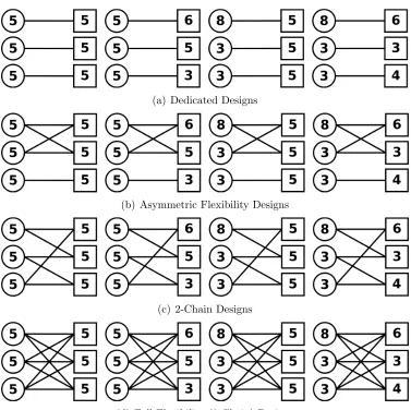
settings. Within each flexibility design setting four problems are considered, each defined by the production capacities of factories,Cf, given in each circle and the inventory capacities of

products, Ip, given in each square. The one-period expected demand, ηp, is set equal to Ip.

Holding costs and penalty costs are set to hp = 1 and θp = 7, respectively, for 1≤ p ≤ P.

Unit factory production costs production costs are set to

uf,p =



 

1.0 1.1 1.21 1.21 1.0 1.1

1.1 1.21 1.0





. (12)

Production costs differ for each factory-product pair due to different technologies, space capabilities and employees at each factory and include variations in transportation costs

Algorithm 2 Q-learning TD(λ) ADP algorithm with -greedy exploration and exploring starts

1: STEP 1: Initialization

2: Initialize ˆV(i) =k ∀ i∈ I

3: Initializee(i) = 0 ∀ i∈ I

4:

5: for m = 1 to M do

6: Choose an initial state i

7: for n= 1 to N do

8: STEP 2: Action Selection

9: Generate random numberx from Uniform[0,1]

10: if x <1−then

11: aˆ←argmin

a n

Ra

i +γ

P

i0β_i,ia0Vˆ(i0) o

12: else

13: aˆ←a random action

14: end if

15:

16: STEP 3: Observe System Feedback

17: Observe random demand, dp ∀ p∈P

18: Observe successor state i0 and immediate cost ˆr

19:

20: STEP 4: Value Function Update

21: v ←rˆ+γVˆ(i0)

22: δ←v−Vˆ(i)

23: e(i)←1

24: Update ˆV(i), e(i) ∀i∈ I by

25: Vˆ(i)←Vˆ(i) +αδe(i)

26: e(i)←γλe(i)

27:

28: STEP 5: Move to Next Iteration

29: i←i0 ∀ p∈P

30:

31: end for

(12)

(a) Dedicated Designs

(b) Asymmetric Flexibility Designs

(c) 2-Chain Designs

[image:12.612.104.481.44.420.2]

(d) Full Flexibility (3-Chain) Designs

Figure 2: Flexibility designs and problem settings used for numerical computations. At each design level problems are distinguished by their production capacities (circles) and inventory capacities (squares).

from factories to each product depot or market.

(13)

Problem Design

C1-C2-C3 I1-I2-I3 Dedicated 2-Chain Full Asymmetric

5-5-5 5-5-5 292.664 278.266 277.820 285.579 5-5-5 6-5-3 294.827 257.737 257.611 280.447 8-3-3 5-5-5 433.580 293.813 293.568 355.562 8-3-3 6-3-4 279.217 243.919 243.895 274.406 Computation times of

[image:13.612.83.493.52.206.2]

DP 0.5 hrs 30 hrs 16 days 20 hrs ADP 4 - 5 mins 2 - 4 hrs 10 - 14 hrs 2 - 3.5 hrs

Table 1: Optimal costs of each flexibility design for each problem setting with typical com-putation times for DP and ADP algorithms

requirements and expected lost sales and that, as shown here, optimal production plans can realise such benefits over time.

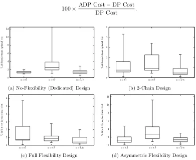
In the main part of the study we wish to identify strongly and poorly performing settings in ADP algorithms. We directly compare the results of the simulated policy performance against DP using the percentage difference in the expected long-run discounted costs via

100× ADP Cost−DP Cost

DP Cost .

0 2 4 6 8 10 12

α = 0.1 α = 0.5 α = 1/n

% difference from optimal cost

No-Flexibility (Dedicated) Design

(a) No-Flexibility (Dedicated) Design

0 1 2 3 4 5

α = 0.1 α = 0.5 α = 1/n

2-Chain Design

(b) 2-Chain Design

0 1 2 3 4 5 6

α = 0.1 α = 0.5 α = 1/n

Full Flexibility Design

(c) Full Flexibility Design

0 2 4 6 8 10 12

α = 0.1 α = 0.5 α = 1/n

Asymmetric Flexibility Design

(d) Asymmetric Flexibility Design

[image:13.612.90.481.371.689.2]

(14)

0 2 4 6 8 10 12

λ = 0 λ = 0.2 λ = 0.5 λ = 0.8 λ = 1

0 1 2 3 4 5

λ = 0 λ = 0.2 λ = 0.5 λ = 0.8 λ = 1

2-Chain Design

(b) 2-Chain Design

0 1 2 3 4 5 6

λ = 0 λ = 0.2 λ = 0.5 λ = 0.8 λ = 1

0 2 4 6 8 10 12

λ = 0 λ = 0.2 λ = 0.5 λ = 0.8 λ = 1

[image:14.612.89.482.50.314.2]

Figure 4: Boxplots of percentage difference in costs between ADP policies and optimal policies for λ={0,0.2,0.5,0.8,1}.

Due to the large number of settings required in the evaluation of the ADP algorithms we split the following analyses into two sections to better focus on the various settings considered. To do so effectively we fix certain settings that have been found to perform well from an earlier study. In the first experiments we fix the initialization of values functions to zero (k = 0), utilise theQ-learning control method with -greedy action selection (= 0.05) and the ADP algorithm runs for 2,000 iterations. With these set we present the results for choices of the step-size parameter α = {0.1,0.5,1/n} (Figure 3); eligibility trace decay

λ = {0,0.2,0.5,0.8,1} (Figure 4); and eligibility traces update method: accumulating or replacing traces (Figure 5). A total of 3×5×2 = 30 setting combinations applied to the 16 problems.

As would be expected, in Figure 3, constant step-sizes exhibit weaker performance in general than the dynamic step-size rule. High constant α = 0.5 is the most inappropriate in this domain with low constant α= 0.1 performing consistently in problems with no flex-ibility structure. The performance under constant step-sizes highlights the influence of the most recent demand samples on the value function updates and, ultimately, the resulting policy. The dynamic step-size rule exhibits the most consistent performance. Strongly per-forming settings for the eligibility trace decay are for low-medium settings, λ={0,0.2,0.5}

(15)

0 2 4 6 8 10 12

Replacing Traces Accumulated Traces

0 1 2 3 4 5

2-Chain Design

(b) 2-Chain Design

0 1 2 3 4 5 6

0 2 4 6 8 10 12

[image:15.612.89.480.50.316.2]

Figure 5: Boxplots of percentage difference in costs between ADP policies and optimal policies for two eligibility trace update rules.

function update than costs incurred later in the simulation. This problem consequence also impacts the choice of eligibility trace update method with the replacing traces method seen to provide more reliable performance than accumulating traces (Figure 5). Many visits to a zero inventory position from high demand for products, for accumulating traces, will result in a high eligibility trace value. If the simulation (randomly) experiences a low cost realisa-tion in that state a negative temporal difference δ will occur. Compounded with the high eligibility trace the update significantly reduces the value function estimate for that state. Greedy action selection will then be attracted to that state which can be accomplished by producing nothing. Even with-greedy action selection an ADP algorithm can struggle move away from a limited number of actions with accumulated traces.

In the second set of experiments we fix to settings with reliable performance from the first experiments and explore other setting choices. We fix to the dynamic step-size parameter

α = 1/n, a low-medium eligibility trace decay λ = 0.2 with the replacing traces method. Again, the ADP Algorithms are run for 2,000 iterations. We present the results for choices of value function initialization k = {0,200,400} (Figure 6); policy selection setting =

{0,0.05,0.1} (Figure 7); control method: Q-learning or SARSA (Figure 8); and simulation path choice: single episode or 20 episodes of 100 iterations each (Figure 9). A total of 3×3×2×2 = 36 setting combinations applied to the 16 problems.

(16)

0 2 4 6 8 10 12

k = 0 k = 200 k = 400

0 5 10 15 20

k = 0 k = 200 k = 400

2-Chain Design

(b) 2-Chain Design

0 5 10 15 20

k = 0 k = 200 k = 400

0 2 4 6 8 10 12

k = 0 k = 200 k = 400

[image:16.612.92.480.49.316.2]

Figure 6: Boxplots of percentage difference in costs between ADP policies and optimal policies for three function initialization choices k ={0,200,400}.

0 0.5 1 1.5 2 2.5

ε = 0 ε = 0.05 ε = 0.1

0 0.2 0.4 0.6 0.8 1 1.2 1.4 1.6 1.8

ε = 0 ε = 0.05 ε = 0.1

2-Chain Design

(b) 2-Chain Design

0 0.5 1 1.5 2

ε = 0 ε = 0.05 ε = 0.1

0 0.5 1 1.5 2 2.5

ε = 0 ε = 0.05 ε = 0.1

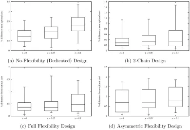
Figure 7: Boxplots of percentage difference in costs between ADP policies and optimal policies for = {0,0.05,0.1} settings. High value function initialization cases (k = 400) excluded.

[image:16.612.90.480.369.636.2]

(17)

0 0.5 1 1.5 2 2.5 SARSA Q-Learning

0 0.2 0.4 0.6 0.8 1 1.2 1.4 1.6 1.8 SARSA Q-Learning

2-Chain Design

(b) 2-Chain Design

0 0.5 1 1.5 2 SARSA Q-Learning

0 0.5 1 1.5 2 2.5 SARSA Q-Learning

[image:17.612.90.481.50.317.2]

Figure 8: Boxplots of percentage difference in costs between ADP policies and optimal policies forQ-Learning and SARSA control policies. High value function initialization cases (k = 400) excluded.

0 0.5 1 1.5 2 2.5

Single Path Exploring Starts

0 0.2 0.4 0.6 0.8 1 1.2 1.4 1.6 1.8

2-Chain Design

(b) 2-Chain Design

0 0.5 1 1.5 2

0 0.5 1 1.5 2 2.5

[image:17.612.90.480.384.649.2]

(18)

Problem Myopic Deterministic ADP

C1-C2-C3 I1-I2-I3 Ded. 2-Chain Full Asymm. Ded. 2-Chain Full Asymm.

[image:18.612.58.522.52.154.2]

5-5-5 5-5-5 14.35 20.47 20.43 17.16 0.70 0.14 1.38 0.68 5-5-5 6-5-3 13.17 22.45 22.46 15.96 0.63 0.32 0.26 0.78 8-3-3 5-5-5 5.68 16.67 16.83 11.83 1.30 0.57 1.64 1.93 8-3-3 6-3-4 14.54 22.82 22.84 16.46 0.75 0.23 0.20 0.27 Table 2: Percentage cost suboptimalities of the myopic-deterministic policy and the resultant policy of the ADP algorithm.

as they move towards their optimal values. Attractive decisions are then to visit such low-cost estimated states (by producing nothing) restricting action exploration by focussing on a limited number of actions, which results in poor policies. Hence, although requiring a longer learning phase, the zero value setting has a more robust performance compared to the positive valued initializations. Presentation of the remaining results will exclude the

k = 400 setting. In Figure 7 we see that high exploration (= 0.1) typically results in higher costs. We comment here that this setting performs the best comparatively for k = 400 where the need to explore the action space is required to overcome the high value function intialisation. However, with an appropriately configured initialization the need to explore actions is lessened. A balanced approach here would be utilise some exploration = 0.05 rather than resort to purely greedy actions (= 0). Figure 8 shows that the control method employed in the problems has little impact in the outcome implying that ease or speed of implementation of the control would be the factor to consider here. Q-learning algorithms, which require smaller number of computations whenV-functions are used, are observed to be slightly faster in these experiments. Similarly, in Figure 9, single or multiple episodes have little impact on performance. The impact of the random demand within the capacitated system, combined with the problem scale, leads to an even distributed state occurrence frequency minimising the need to employ multiple episodes.

We conclude the study with a comparison of the performance of policies derived from an ADP algorithm and a simple myopic deterministic policy. From the experiments above a sensible setting of the ADP algorithm would be a Q-learning algorithm with a replacing traces update method using a single-start simulation path, with parameters set as α= 1/n,

λ= 0.2,k = 0,= 0.05. The myopic deterministic policy is derived by solving a single period optimization problem with deterministic demand for each product set to its mean, ηp. This

(19)

5 Conclusions

An important aspect of the investigative study of the previous section is that implications of problem design and structure greatly affect appropriate settings and choices in the construc-tion of ADP algorithms. Such findings can drive the extension of ADP algorithms to similar problems of greater size and complexity. From inspection of optimal policies resulting from DP value iteration we can confirm that, as one might think naturally, production decisions are (dynamically) of threshold-type. The capacity requirements of production and inventory also have a strong influence. The nature of state aggregation this engenders results in re-generative states at these limits, which implies that an average cost per unit time objective would also be viable and therefore worthy of consideration.

Our numerical study reveals relations between a number of settings (value function initial-ization, eligibility trace decay value and eligibility trace update method) and the assumptions of capacitated production and no back-ordering in our process flexibility problem. This pro-vides an important insight on how to adjust these settings for any problem size. Without foreknowledge of optimal value functions a zero-value function initialization (k = 0) is shown to perform well. Complimentary to that is the use of low eligibility trace settings (λ) and the application of replacing traces. Inappropriate choices for these settings in any problem size may result in poorly performing algorithms due to the state aggregation effects.

For the remaining settings investigated, our numerical study provides valuable clues on how ADP algorithms performed compared to optimal under different parameter settings and where to search for appropriate settings in larger scale problems. With the stationary problem setting and implied state aggregation a simple dynamic step-size setting (α= 1/n) is observed to work well. To balance the issue of ADP algorithms possibly restricting to a limited number of actions and states some small amount of exploration is recommend through -greedy exploration with = 0.05, say. For the tractable look-up table problems considered here, the choice between using a single-start simulation path and exploring starts or which policy control method has little impact on the performance of the resulting policy. Hence, such a decision can be restricted to the ease or speed of implementation.

The ADP look-up table approach still requires allocating memory for the entire state space and can involve calculating cost-to-go expectations of actions for a given state to find the best action amongst them. We note that, although requiring less computational time, allocating memory for the state space and calculating expectations even for a single action is still not feasible for large multidimensional systems. The challenge to a broader implementation is in extending to problems for which the memory constraints render a look-up table approach infeasible. One could clearly adapt the work of Wu et al. (2016) to develop effective solutions to this problem. The black-box nature ANN results in a functional form of value function that still requires the optimization of the ADP equivalent of the r.h.s. of (2) to realise the resulting action. Evaluation of such could require recourse to heuristic optimization techniques which will add an additional computational burden. An alternative approach would be to consider a parametric representation of the value functions, utilising knowledge of the threshold-type optimal policies and the impact of ongoing costs resulting from high and low inventory states respectively. Design of a parametric form that is tractable to exact optimization techniques for (greedy) action selection would be valuable due to both the speed of implementation and transparency of the value function estimations.

(20)

costs, treating them as separate entities may yield useful managerial insights. Another chal-lenging progression would be to investigate the effects of positive production lead times and stochastic production output in process flexibility problems. With respect to the change in inventory costs, (close to) optimal policies and benefits of investing in process flexibility could be developed.

Acknowledgements

The authors would like to thank the two anonymous reviewers for their constructive com-ments that helped to improve the presentation of this paper.

Disclosure statement

No potential conflict of interest was reported by the authors

References

C¸ imen, M. and C. Kirkbride (2013). Approximate dynamic programming algorithms for multidimensional inventory optimization problems. IFAC Proceedings Volumes 46(9), 2015 – 2020.

Chou, M. C., G. A. Chua, and C.-P. Teo (2010). On range and response: Dimensions of process flexibility. European Journal of Operational Research 207(2), 711 – 724.

Chou, M. C., C. P. Teo, and H. Zheng (2008). Process flexibility: Design, evaluation, and applications. Flexible Services and Manufacturing Journal 20, 59–94.

Deng, T. and Z. J. M. Shen (2013). Process flexibility design in unbalanced networks.

Manufacturing & Service Operations Management 15(1), 24–32.

Francas, D., M. Kremer, S. Minner, and M. Friese (2009). Strategic process flexibility under lifecycle demand. International Journal of Production Economics 121(2), 427–440. George, A. P. and W. B. Powell (2006). Adaptive stepsizes for recursive estimation with

applications in approximate dynamic programming. Machine Learning 65(1), 167–198. Gustavsson, S. O. (1984). Flexibility and productivity in complex production processes.

International Journal of Production Research 22(5), 801–808.

He, P., X. Xu, and Z. Hua (2012). A new method for guiding process flexibility investment: Flexibility fit index. International Journal of Production Research 50(14), 3718–3737. Jain, A., P. K. Jain, F. T. S. Chan, and S. Singh (2013). A review on manufacturing

flexibility. International Journal of Production Research 51(9), 5946–5970.

(21)

Kunnumkal, S. and H. Topaloglu (2008). Using stochastic approximation methods to com-pute optimal base-stock levels in inventory control problems.Operations Research 56(3), 646–664.

Lewis, F. L. and D. Liu (2013). Reinforcement learning and approximate dynamic

program-ming for feedback control, Volume 17. John Wiley & Sons.

Liu, D., X. Yang, and H. Li (2013). Adaptive optimal control for a class of continuous-time affine nonlinear systems with unknown internal dynamics. Neural Computing and

Applications 23(7-8), 1843–1850.

Nascimento, J. and W. B. Powell (2013). An optimal approximate dynamic programming algorithm for concave, scalar storage problems with vector-valued controls.IEEE

Trans-actions on Automatic Control 58(12), 2995–3010.

Ni, Z., H. He, D. Zhao, X. Xu, and D. V. Prokhorov (2015). Grdhp: A general utility function representation for dual heuristic dynamic programming. IEEE transactions on

neural networks and learning systems 26(3), 614–627.

Powell, W. B. (2007). Approximate Dynamic Programming: Solving the Curses of

Dimen-sionality (1 ed.). John Wiley and Sons, Inc.

Rafiei, H., M. Rabbani, H. Vafa-Arani, and G. Bodaghi (2016). Production-inventory analy-sis of single-station parallel machine make-to-stock/make-to-order system with random demands and lead times. International Journal of Management Science and Engineering

Management To Appear(doi: 10.1080/17509653.2015.1113393).

Sethi, A. K. and S. P. Sethi (1990). Flexibility in manufacturing: A survey.The International

Journal of Flexible Manufacturing Systems 2, 289–328.

Sharaf, I. M. (2016). A projection algorithm for positive definite linear complementarity problems with applications. International Journal of Management Science and

Engi-neering Management To Appear(doi: 10.1080/17509653.2015.1132643).

Simchi-Levi, D. and Y. Wei (2015). Worst-case analysis of process flexibility designs.

Oper-ations Research 63(1), 166–185.

Soysal, M. (2016a). Closed-loop inventory routing problem for returnable transport items.

Transportation Research Part D To Appear(doi: 10.1016/j.trd.2016.07.001).

Soysal, M. (2016b). A research on non-stationary stochastic demand inventory systems.

International Journal of Business and Social Science 3(7), 153–158.

Sutton, R. S. and A. G. Barto (1998). Reinforcement Learning: An Introduction (1 ed.). Cambridge, Masachusetts, MIT Press.

Tanrisever, F., D. Morrice, and D. Morton (2012). Managing capacity flexibility in make-to-order production environments. European Journal of Operational Research 216(2), 334–345.

Tarim, S. A. and B. G. Kingsman (2004). The stochastic dynamic production/inventory lot-sizing problem with service-level constraints. International Journal of Production

(22)

Topaloglu, H. and S. Kunnumkal (2006). Approximate dynamic programming methods for an inventory allocation problem under uncertainty. Naval Research Logistics 53(8), 822–841.

Van Roy, B., D. P. Bertsekas, D. P. Lee, and J. N. Tsitsikilis (1997). A neuro-dynamic programming approach to retailer inventory management. In Proceedings of the 36th

IEEE Conference on Decision and Control,, Volume 4, pp. 4052–4057.

Wu, H., G. Evans, and K.-H. Bae (2016). Production control in a complex production system using approximate dynamic programming. International Journal of Production

Research 54(8), 2419–2432.

Yang, X., D. Liu, and Q. Wei (2014). Online approximate optimal control for affine non-linear systems with unknown internal dynamics using adaptive dynamic programming.