Boundedly rational expected utility theory
Daniel Navarro-Martinez1,2&Graham Loomes3&Andrea Isoni3,4& David Butler5&Larbi Alaoui1,2
Published online: 28 December 2018 #The Author(s) 2018
Abstract
We build a satisficing model of choice under risk which embeds Expected Utility Theory (EUT) into a boundedly rational deliberation process. The decision maker accumulates evidence for and against alternative options by repeatedly sampling from her underlying set of EU preferences until the evidence favouring one option satisfies her desired level of confidence. De-spite its EUT core, the model produces patterns of behaviour that violate standard EUT axioms, while at the same time capturing systematic relation-ships between choice probabilities, response times and confidence judgments, which are beyond the scope of theories that do not take deliberation into account.
Keywords Expected utility . Bounded rationality . Deliberation . Probabilistic choice . Confidence . Response times
JEL Classifications D03 . D81
Electronic supplementary materialThe online version of this article ( https://doi.org/10.1007/s11166-018-9293-3) contains supplementary material, which is available to authorized users.
* Daniel Navarro-Martinez [email protected]
* Graham Loomes
1
Department of Economics and Business, Pompeu Fabra University, Ramon Trias Fargas 25-27, 08005 Barcelona, Spain
2 Barcelona Graduate School of Economics, Barcelona, Spain
3
Warwick Business School, University of Warwick, Coventry CV4 7AL, UK
4
University of Cagliari, Cagliari, Italy
5
1 Introduction
Economics is often said to be the study of the allocation of scarce resources, of how human beings decide to combine their time and skills with physical resources to produce, distribute and consume. However, economic models may sometimes ignore the fact that arriving at decisions is itself an economic activity and that the hardware and software involved—that is, the human brain and its mental processes—are themselves subject to constraints. Herbert Simon emphasised this point in his 1978 Richard T. Ely lecture, in which he discussed the implications of attention being a scarce resource.1 In a world where there are many (often complex) choices to be made, spending time on any one decision entails an opportunity cost in terms of the potential fruits of other decisions that might have been considered instead. Being unable to devote unlimited time and attention to every decision they encounter, humans generally have to satisfice rather than optimise.
Simon bemoaned the lack of interest among economists in the processes that individuals use when deciding how to allocate their scarce mental resources, and he advocatedBbuilding a theory of procedural rationality to complement existing theories of substantive rationality^. He suggested thatBsome elements of such a theory can be borrowed from the neighboring disciplines of operations research, artificial intelligence, and cognitive psychology^, but noted that Ban enormous job remains to be done to extend this work and to apply it to specifically economic problems^ (Simon1978, pp.14–15).
Although there have been some developments along these lines (e.g., Gilboa and Schmeidler 1995; Rubinstein 1988; Gigerenzer and Selten 2001), the decades that followed Simon’s lecture saw the mainstream modelling of indi-vidual decision making—especially with respect to choice under risk and uncertainty—take a different direction. Stimulated by experimental data that appeared to violate basic axioms of rational choice, a number of models appeared at the end of the 1970s and in the early 1980s that sought to provide behavioural alternatives to standard Expected Utility Theory (EUT)—see Starmer (2000) for a review. Typically, these were deterministic models that relaxed a particular axiom and/or incorporated various additional features—e.g., reference points, loss aversion, probability weighting, regret, disappointment—to try to account for certain regularities in observed decisions. While such models provided more elaborate descriptive theories of choice, little or no consideration was given to the mental constraints referred to by Simon. His invocation to build boundedly rational procedural models largely fell by the wayside in the field of risky decision making.
Thus we now have an impressive array of alternative deterministic models, each of which can claim to accommodate some (but not all) of the observed departures from EUT. However, these models have no intrinsic explanation for
at least three other pervasive empirical regularities in the data, which may arise from features of the decision-making process: first, the probabilistic nature of most people’s decisions2; second, the systematic variability in the time it takes an individual to respond to different decision tasks of comparable complexity3; and third, the degree of confidence decision makers (DMs) express about their decisions.4
In this paper, we propose to explore the direction Simon advocated and investigate the potential for applying a boundedly rational deliberative process to the ‘industry standard’ model of decision making under risk and uncertainty, EUT. We start by identifying in general terms what is required of a procedural model of preferential choice. We then consider how the various components of such a model might be specified in ways that are in keeping with conventional economic assumptions while at the same time allowing for scarcity of time and attention. The resulting model—which we call Boundedly Rational Expected Utility Theory (BREUT)—generates a number of implications, not just about choice probabilities, but also about process measures such as response times and confidence in the decisions made.
One striking result is that, despite being based upon EU preferences, the model produces some choice patterns that deviate from EUT in line with several well-known decision-making phenomena. This highlights the influence of the processes that lead from the ‘core’ assumptions about preferences to observable choices. At the same time, there are other choice patterns that are not accommodated by BREUT. So we are not proposing BREUT as a descrip-tive model that can account for all known empirical regularities; nor is it intended to provide a literal representation of the way the mind actually operates. Rather, this paper may be understood as a‘proof of concept’ exercise, which demonstrates the implications of embedding a deterministic core in a simple boundedly rational apparatus to generate decisions. As we shall explain in due course, our broad modelling strategy has the potential to be extended to many non-EU core theories, some of which may accommodate more or other known regularities.
In the next section, we present our instantiation of BREUT, focusing upon the kind of binary choices between lotteries with monetary outcomes that have been the staple diet of many decision-making experiments. In Section 3, we demonstrate how BREUT provides a parsimonious account of the systematic relationship between choice probabilities, decision time and confidence. We show that the model entails respect for first order stochastic dominance and weak stochastic transitivity, but allows patterns of choice that violate strong
2When participants are presented with exactly the same decision task displayed in exactly the same way on two or more separate occasions within the same experiment, they often give different responses on different occasions. See Mosteller and Nogee (1951) for an early example; Luce and Suppes (1965) for a review of the early theoretical literature; and Rieskamp et al. (2006), Bardsley et al. (2010, Chapter 7), and Baucells and Villasís (2010) for more recent discussions.
3See, for example, Tyebjee (1979), Birnbaum and Jou (1990), Busemeyer and Townsend (1993), Wilcox (1993), Moffatt (2005), Rubinstein (2007,2013), Spiliopoulos and Ortmann (2016), Achtziger and Alós-Ferrer (2014).
4
stochastic transitivity, independence and (to some extent) betweenness. In the final section, we consider the relationship between our model and others in the psychology and economics literature. We discuss some limitations of the model in its current form, together with what we see as the most promising directions for extending this approach. Some theorems and their proofs can be found in the online appendix.
2 The model
Bounded rationality has often been characterised in terms of the difficulties DMs may encounter when they are faced with complex problems or environ-ments involving information that is hard to obtain and compute. However, we suggest that bounded rationality may play a role even for relatively simple decisions. Even when there are just two options, the DM will need to identify and evaluate the arguments pulling in opposing directions. Because the DM cannot dwell on a decision indefinitely, she will need some mechanism to decide when to terminate her deliberation and move to a different task. It is the process underlying the allocation of time and attention between different decisions that we regard as fundamental to the characterisation of bounded rationality.
Behavioural scientists have invested substantial effort in developing various approaches for modelling decision-making processes: see, for example, elimi-nation by aspects (Tversky 1972); the adaptive decision maker framework (Payne et al. 1993); the priority heuristic (Brandstätter et al. 2006); and query theory (Johnson et al. 2007), to name only a few. An influential stream of literature has developed an accumulator or sequential-sampling framework (for reviews, see Ratcliff and Smith 2004; Otter et al. 2008). Most such accumulator models have been developed in the context of perceptual tasks (e.g., judging the relative numbers of dots in different areas of a screen or the relative lengths of lines). The application of these models to preferential choice has been less common, although Busemeyer and Townsend’s (1993) Decision Field Theory (DFT) and its extensions constitute a notable exception. BREUT draws on this accumulator framework, and we will discuss its relationship with DFT in more detail in Section 4.
Such models typically consist of three components:
(i) some representation of the sources of evidence from which samples are drawn—in this context, the underlying stock of subjective values or judgments;
(ii) some account of the way the sampled evidence is accumulated;
(iii) a stopping rule which terminates the accumulation process and triggers a decision.
In the next three subsections, we explain how BREUT models these three components. In each case, we try to make the simplest possible assumptions.
2.1 The structure of underlying subjective values
We will be concerned with choices between pairs of lotteries of the formL= (x1,p1;x2,
p2; …; xn, pn), where consequence xi occurs with probability pi, ∑ni¼1pi¼1. In
deterministic EUT, DMs are assumed to choose the lottery for which∑ni¼1piu xð Þi is
higher, whereu(.) is a von Neumann-Morgenstern (vNM) utility function.
Let us start with the following seemingly simple decision. A DM is asked to choose between lotteryA, which (omitting any currency symbol) offers the certainty of 30, and lotteryB, which offers a 0.8 chance of 40 and a 0.2 chance of 0. Using standard EUT notation, with≽denoting weak preference, the decision can be written as:
A≽B⟺uð Þ30 ≥ 0:8uð Þ þ40 0:2uð Þ0 : ð1Þ
Deterministic EUT supposes that it is as if each DM acts according to a single utility function that gives an exact answer to this question (and gives the same answer every time that this question is presented to her). But cognitive psychology and neuroscience suggest that there is no unique and instantly accessible subjective value function—see, for example, Busemeyer and Townsend (1993), Gold and Shadlen (2007), Stewart et al. (2006,2015). Rather, a typical DM will have many experiences and impressions of what 30 and 40 represent in subjective terms, and it may not be immediately obvious exactly where the subjective value of 30 is located in the range between the subjective values of 0 and 40, nor precisely how the differences, weighted by the probabilities, balance out. So arriving at a decision may involve deliberating about the balance of evidence obtained by sampling from those experiences and impressions.
Since we are investigating the effects of embedding EUT in a boundedly rational deliberation process, we represent the underlying stock, orcore, of past experiences and impressions by a distribution of vNM utility functions, u(.), normalised so that u(0) = 0.
2.2 Modelling the sampling and accumulation of evidence
Adapting the general framework of accumulator models to the specific context of binary choice between lotteries, BREUT models each sample as an independent random draw of a utility function from the core distribution ofu(.), which is then applied to both of the lotteries under consideration. Using probabilities as weights, as EUT entails, this yields a subjective value difference which we denote byV(A,B), and which takes some positive value when au(.) is drawn that strictly favoursA, takes a value of zero when the two options are exactly balanced, and takes a negative value when the sampledu(.) strictly favours B. We can represent this difference as a difference between the monetary certainty equivalents (CEs) of the two options. Formally, for anyu(.) sampled,
V Að ;BÞ ¼CEA−CEB¼u−1ðEUAÞ−u−1ðEUBÞ: ð2Þ
We use differences inCEs rather than in utilities becauseCEs are measures that can be legitimately compared and aggregated across utility functions. It is well known in economics that comparisons of utilities (or their aggregation) across different utility functions are theoretically questionable and lead to problematic results (e.g., Hammond
1993; Binmore2009). For this reason, we putV(A,B) in a‘common metric’that can be legitimately aggregated. The use ofCEs is a straightforward way of achieving that and has a number of precedents in the literature (e.g., Luce1992; Luce et al.1993; Cerreia-Vioglio et al.2015).
For each sampledu(.), theCEdifference provides a signal not only about which option is better, but also about how much better it is. Repeated sampling (with replacement) produces a series of independently and identically distributed realisations
of V(A,B), which are accumulated by progressively updating their mean and sample
standard deviation, denoted respectively byV Að ;BÞandsV(A,B).
Let E[V(A,B)] denote the mean of the distribution ofCEdifferences for the pair of lotteries {A, B} implied by the individual’s underlying population of u(.). If the individual takes a sample of sizekfrom this distribution, that sample will have a mean which we denote byVkðA;BÞ. Taking sufficiently many samples of sizekwill result in
some distribution forVkðA;BÞ. Askbecomes larger, the distribution ofVkðA;BÞwill
be increasingly similar to a normal distribution with a variance inversely related tok. If the individual were to deliberate indefinitely—that is, ifkwere allowed to tend towards infinity—the variance of the distribution ofVkðA;BÞwould tend towards zero and the
2.3 Modelling the stopping rule
Unlike other accumulator models in which the process of evidence accumulation terminates when an arbitrary threshold is reached, we propose an approach which sets thresholds that are responsive both to the evolving pattern of the evidence as it accumulates and to the DM’s wish to limit the time spent deliberating about any particular decision. The key to our stopping rule is the DM’sdesired level of confi-dence: the DM deliberates until she concludes that the accumulated evidence gives her sufficient confidence to make a choice. In BREUT, confidence is represented as the probability that the DM picks the option that she would choose after unlimited deliberation—i.e., the option implied by the sign of E[V(A,B)].
We suggest that the notion of an individual attempting to achieve a personal desired level of confidence is a simple and intuitive way of building a satisficing model, and also one for which there is some empirical support (see Hausmann and Läge2008). In contrast with the optimal stopping tradition (see, e.g., Stigler1961; Shiryaev1978), this approach does not require us to assume that the individual has detailed knowledge about the opportunity cost of additional sampling in terms of forgone benefits from potential future activities.
We denote the DM’s desired level of confidence asConf. Because deliberation is costly in terms of the opportunity costs associated with each extra draw, we allow the DM to progressively reduceConfas the amount of sampling increases. The idea here is that the longer she spends trying to discriminate between options, the more likely she is to conclude that there is not much between them, so that she has less to fear from choosing the wrong option. Specifically, we assume that the desired level of confidence afterkdraws is given by:
Conf ¼max 0½ :5;1−d kð −1Þ; ð3Þ
wherek≥2 and whered(with 0 <d≤0.5) is a parameter that captures the rate at which the DM reduces herConfaskincreases, subject to the constraint thatConf≥0.5.
dmay vary from one individual to another, reflecting different tastes for the trade-off between more input into the current decision and turning attention to something else. A person with a very lowdis someone who wants to be very confident in her decisions, and therefore is willing to invest more time deliberating. The limiting case is whend→ 0, in which the individual wants to be absolutely sure of making the right decision and deliberates indefinitely. On the other hand, someone with a high value ofdis ready to make decisions with less confidence and spends relatively less time deliberating. Thus whend has the maximum value of 0.5, the DM makes her decision after just two samples, choosing the option favoured by the mean of the two sampledCEdifferences. Modellingdas a personal characteristic provides a degree of within-person consistency with just one parameter, while allowing for heterogeneity between people. It would be possible to construct a more complicated function for Conf, but the linear form in Expression3is sufficient for our‘proof of concept’purposes.
well with the idea of achieving some personal level of confidence. What we try to capture is the idea that when the choice is initially presented—i.e., before any delib-eration has occurred—it is as if the DM starts with the null hypothesis that there is no significant difference between the subjective values of the two options. However, as the evidence accumulates, it is as if she continually updates V Að ;BÞ and sV(A,B) and
combines them to form a test statisticTk:
Tk¼
V Að ;BÞ sV Að ;BÞ=
ffiffiffi
k
p : ð4Þ
This statistic is then used to determine whether the null hypothesis of zero difference can be rejected at the level ofConfcorresponding tok. This occurs if the following condition is met:
Fk−1½absð ÞTk ≥Conf; ð5Þ
whereFk–1[·] is the c.d.f. of the t-distribution withk–1 degrees of freedom. If the
weak inequality in Expression 5 is not satisfied, the DM is assumed to continue sampling and to progressively reduce Conf until the hypothesis of zero difference between the options is rejected in favour of one of the alternatives—at which point, she chooses whichever option is favoured by the evidence according to the sign of V Að ;BÞ. The value ofkwhen sampling stops and a choice is made is denoted byk*, the level of confidence at that point isConf* and the value of the test statistic at that point isTk*.
2.4 Behavioural variables generated by BREUT
Because of its procedural nature, BREUT gives a richer description of decision making than process-free models, as captured by the following three variables: choice proba-bilities, confidence and response times. We now consider each of these in more detail.
2.4.1 Choice probabilities
In BREUT, the probability of choosingAoverB, denoted by Pr(A≻B), is the probability that the null hypothesis is rejected with a positiveTk*. The complementary probability
thatBis chosen is the probability that the null hypothesis is rejected with a negativeTk*.
In the classic RP model, it is as if an individual samples just once per decision and chooses on the basis of the singleu(.) sampled on that occasion. In that one-shot model, the probability of choosingAoverBis given by the proportion of utility functions that favourAoverBin the underlying core distribution. We denote this probability by Pr
Core(A≻B). However, BREUT supposes that an individual samples more than once, so
B)] askbecomes larger. As a consequence, askincreases, the DM becomes increas-ingly likely to choose the option favoured by the sign of E[V(A,B)]. In the limit, the probability of choosingAoverBasktends towards infinity, denoted by PrLim(A≻B), is either 0 (if E[V(A,B)] is negative) or 1 (if E[V(A,B)] is positive). This means that:
0¼PrLim Að ≻BÞ≤PrðA≻BÞ≤PrCore Að ≻BÞ ifE V A½ ð ;BÞ<0
PrCore Að ≻BÞ≤PrðA≻BÞ≤PrLim Að ≻BÞ ¼1 ifE V A½ ð ;BÞ>0: ð6Þ
That is, Pr(A≻B) always lies between the core probability in the one-shot RP model and the limiting probability (0 or 1) implied by the sign of the mean of the distribution of CEdifferences.
Expression6has some important implications. First, if one of the lotteries is never favoured by the individual’s core utility functions (i.e., PrCore(A≻B) is either 0 or 1), then there will be no amount of sampling for which that lottery will be chosen with positive probability (i.e., it will always be the case that Pr(A≻B) = PrCore(A≻B) = Pr Lim(A≻B)). Since dominated lotteries are never chosen in EUT, this entails that BREUT satisfies first-order stochastic dominance. Second, since (other things being equal) lower values ofd imply larger values ofk*, Pr(A≻B) will tend towards PrLim(A≻B) asd decreases: in other words, with more deliberation, choice probabilities become more extreme. Third, if PrLim(A≻B) and PrCore(A≻B) are on different sides of 0.5 for some core, then BREUT allows for one lottery to be the modal choice even though the majority of the DM’s core utility functions favour the other lottery (see Section3.3and Theorems 1 and 3 in theonline appendix).
2.4.2 Confidence
In BREUT, the degree of confidence in a decision,Conf*, is the level ofConfused in the test that rejects the null hypothesis and triggers a choice in favour of one of the alternatives afterk*samples.
While a substantial literature has investigated and modelled confidence judgments in decision tasks that have a correct answer (see Pleskac and Busemeyer 2010, and references therein), there are only a few isolated exceptions of studies investigating confidence judgments in preferential choice (e.g., Butler and Loomes1988; Sieck and Yates1997). Whereas response times and choice probabilities are directly observable, confidence is a latent variable that is typically elicited by asking people about it, which can be done in a variety of ways (e.g., Koriat et al.1980; Koehler1991; Griffin and Tversky1992). To the best of our knowledge, there are no other decision models that explicitly address confidence in preferential decisions, although confidence is clearly regarded as an important factor in various areas of economics (e.g., Acemoglu and Scott1994; Ludvigson2004; Dominitz and Manski2004; Barsky and Sims2012).5
5
2.4.3 Response time
Since deliberation is modelled through sequential sampling, BREUT can make predic-tions about the length of time that it takes to make a decision—theresponse time(RT). It is reasonable to assume thatRTis an increasing function of the number of samples, k*, required to reject the null hypothesis. In addition,RTcan also be expected to be positively related to the complexity of the decision problem. As there is no generally agreed index of complexity for such choices, for the purposes of this paper we make the simple assumption that complexity is reflected by the total number of consequences (NC) appearing in any pair.6This is a straightforward way of capturing the intuition that, if there are more items to consider, each deliberation step will take longer. So we propose the following basic specification forRT:
RT ¼k*∙NC: ð7Þ
Sincek*is a stochastic variable,RTis also stochastic, implying that the DM is liable to take different amounts of time to reach a decision for the same pair of alternatives on different occasions. Given Expression3and the definition ofk*, it follows thatRT= [(1–
Conf*)/d+ 1]NC. That is,RTandConf*are inversely related. Also, we assume thatRT
only depends on the other parameters of the model and is not directly affected by any other contextual features. In practice, the magnitude of response times is likely to be affected by other factors, such as the particular ways in which the alternatives are displayed, the time needed to scan the stimuli, the respondent’s familiarity with the nature and format of the task, her degree of fatigue and so on. More elaborate expressions could be constructed to allow for such considerations, including a scaling factor that mapsRTs to real time if the model is to be fitted to data, but Expression7is adequate for our immediate purposes.
3 Exploring the predictions of BREUT
To explore the predictions of BREUT as a function of its parameters, we conducted simulations in which the utility functions are assumed to be drawn from a fixed population of power functions of the following form (some theorems for the limiting case ofd→0 can be found in theonline appendix):
U xð Þ ¼x1−r; ð8Þ
withr< 1. ris a random variable that varies from trial to trial, is independently and identically distributed, and can produce risk seeking (r< 1), risk neutrality (r= 0) and risk aversion (0 <r< 1).7
6If the same consequence appears in both alternatives, it is counted twice inNC. If it appears twice in the same alternative, it is counted once.
7
We assume that each time the DM samples from her core preferences, it is as if an r is extracted from a transformed beta distribution of risk attitude parameters, such that:
r∼Beta 3ð ;3Þ∙βþ α−β 2
: ð9Þ
This means that herrvalues are drawn from a symmetric and bell-shaped distribution with meanαand rangeβ, which is bounded below and above atα–β/2 andα+β/2 respectively. Ifβ= 0, the specification reduces to deterministic EUT withr=α.
Using this core structure, we implement the model by making independent random draws of values ofr, each of which entails aCEdifference between the two lotteries under consideration, and we accumulate those differences according to Expression4
until the condition in Expression 5 is met. We simulate this process 20,000 times (unless otherwise stated) for each binary choice to generate choice probabilities, mean RTs and averageConf*.8
In the rest of the section, we examine how the model behaves in three respects. First, we show the results of comparing a fixed lottery to a monotonic sequence of sure alternatives when we hold the parameters of the model constant. Second, we explore how changes in each ofα, β and d affect BREUT’s predictions when we hold the alternatives constant. Third, we use more specific sets of decision problems to illustrate how BREUT behaves in scenarios involving stochastic dominance, transitivity, inde-pendence, and betweenness.
3.1 Fixed lottery vs. variable sure amounts
Table1shows how choice probabilities, confidence and response times vary in choices between a fixed lottery and a series of sure amounts of money when we set the parameters atα= 0.35,β= 1.0 andd= 0.1. The fixed lotteryB(shown in the heading of the table) offers a payoff of 40 with probability 0.8 and zero with probability 0.2, represented as (40, 0.8;0, 0.2). The sure amountsA(shown in the first column) increase from 20 to 32 in steps of 2.
As should be expected, increasing the value ofA raises the proportion of utility functions favouringAoverB, so that PrCore(A≻B) rises from 0.04 (whenAis 20) to 0.97 (whenAis 32). For the values ofAfrom 20 to 26 inclusive, the mean of the core distribution ofCEdifferences is negative, as shown in the E[V(A,B)] column, so that Pr
Lim(A≻B) = 0.9 In these cases, repeated sampling moves Pr(A≻B) away from Pr
Core(A≻B) towards 0, as entailed by Expression6. Even when 26% ofu(.) favourA,
as in the fourth row whereA= 26, repeated sampling results inAbeing picked on only 13% of occasions.
However, when A increases to 28, E[V(A, B)] becomes positive, so that Pr Lim(A≻B) = 1 for this and all higher values ofA. This means that for the remaining
8
All simulations and calculations were implemented using R. The code is available from the authors on request.
9
rows in the table, repeated sampling moves Pr(A≻B) above Pr Core(A≻B). As a consequence, even though just 45% ofu(.) favourAwhenA= 28,Ais chosen more often—in this example, in slightly more than 50% of the simulation runs, resulting in
Pr(A≻B) and Pr Core(A≻B) being on different sides of 0.5. When A= 30 and is
favoured by 73% ofu(.), the deliberative process results inAbeing chosen in 92% of runs.
The next two columns show the average RTand the average levels of Conf*. In the rows towards the top and bottom of the table, where one or the other option is strongly favoured, RTs are shorter and Conf* is higher. In the middle rows, where the two options are more finely balanced, more sampling is required to reject the null hypothesis of zero difference, so that RTs become longer and Conf* decreases. This pattern in the RTs is in line with existing empirical evidence for choices between lotteries (see, e.g., Mosteller and Nogee
1951; Jamieson and Petrusic 1977; Petrusic and Jamieson 1978; Moffatt
2005).10 The confidence pattern is in line with the evidence found in perceptual tasks (see Pleskac and Busemeyer 2010, for a review of this literature).
3.2 Changing the free parameters of the model
We illustrate the effect of changingα,βandd, in turn, by simulating choices for the pair {A,B}, withA= (30, 1) andB= (40, 0.8;0, 0.2).
Table2shows that whenα(the mean value ofr) is progressively increased so that the DM becomes more risk averse overall, Pr(A≻B) and Pr Core(A≻B) both increase monotonically, with Pr(A≻B) tending to be more extreme than Pr Core(A≻B), as implied by Expression 6. RTs tend to increase for more finely balanced decisions, while theConf*values show the opposite pattern.
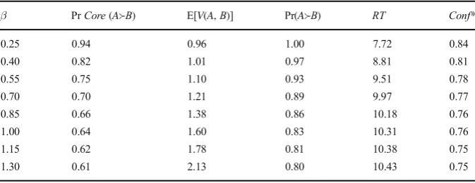
Table 3 shows that, as β is increased (widening the range of r), more sampling is required to trigger a decision, which results in longer RTs and lower confidence.
10
[image:12.439.52.389.81.197.2]The overall distribution ofRTs tends to be positively skewed. This is often observed in experiments (e.g., Ratcliff and Smith2004), even though this evidence typically comes from tasks in which there is a correct answer, as opposed to preferential choice.
Table 1 Choice between a fixed lotteryB= (40, 0.8;0, 0.2) and increasing sure amounts of moneyA(α=
0.35,β= 1.0,d= 0.1)
A PrCore(A≻B) E[V(A,B)] Pr(A≻B) RT Conf*
(20, 1) 0.04 −7.58 0.00 7.02 0.87
(22, 1) 0.08 −5.60 0.00 7.56 0.85
(24, 1) 0.15 −3.60 0.02 8.46 0.82
(26, 1) 0.26 −1.58 0.13 9.90 0.77
(28, 1) 0.45 0.42 0.50 10.99 0.73
(30, 1) 0.73 2.41 0.92 9.63 0.78
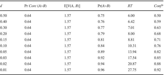
Table4 shows the effect of decreasingd. When d= 0.5 (so that k*= 2), Pr(A≻B) goes from the PrCore(A≻B) level of 0.64 to 0.75 (note that since E[V(A,B)] > 0, Pr
Lim(A≻B) = 1 in this case). At the other extreme, when d= 0.01, Pr(A≻B) is much
closer to the limiting probability of 1. Lower values ofd mean that the DM is less willing to reduce her desired level of confidence, which entails increasing the average amount of sampling and the averageRTs. So in the third row, whered= 0.3, average RTs are 7.01, reflecting the fact that withNC= 3, the averagek*is 2.34; in the sixth row, whered= 0.1,RTs are around 10. TheRTs continue to rise asdfalls further.
3.3 Implications for stochastic dominance, transitivity, independence and betweenness
[image:13.439.51.389.71.201.2]We now apply BREUT to some specific problems which are typical of those used in many experimental studies. We explore the extent to which BREUT’s predictions do or do not correspond with various well-known patterns.
Table 2 Changing the median risk aversion parameterα(β= 1.0,d= 0.1)
α PrCore(A≻B) E[V(A,B)] Pr(A≻B) RT Conf*
0.05 0.20 −1.36 0.05 9.12 0.80
0.10 0.28 −0.87 0.13 10.01 0.77
0.15 0.36 −0.39 0.28 10.73 0.74
0.20 0.45 0.19 0.49 11.01 0.73
0.25 0.55 0.84 0.68 10.84 0.74
0.30 0.64 1.57 0.83 10.32 0.76
0.35 0.73 2.41 0.92 9.65 0.78
0.40 0.80 3.39 0.97 9.01 0.80
A= (30, 1)
[image:13.439.51.388.462.592.2]B= (40, 0.8;0, 0.2)
Table 3 Changing the range of the distribution of risk aversion coefficientsβ(α= 0.30,d= 0.1)
β PrCore(A≻B) E[V(A,B)] Pr(A≻B) RT Conf*
0.25 0.94 0.96 1.00 7.72 0.84
0.40 0.82 1.01 0.97 8.81 0.81
0.55 0.75 1.10 0.93 9.51 0.78
0.70 0.70 1.21 0.89 9.97 0.77
0.85 0.66 1.38 0.86 10.18 0.76
1.00 0.64 1.60 0.83 10.31 0.76
1.15 0.62 1.78 0.81 10.38 0.75
1.30 0.61 2.13 0.80 10.43 0.75
A= (30, 1)
3.3.1 First order stochastic dominance
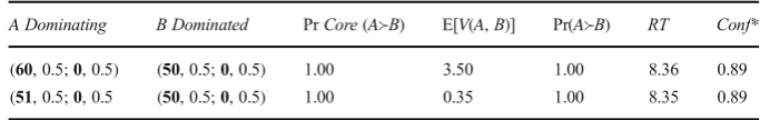
As noted in Section2.4, Expression6entails that whenever one of the lotteries is never favoured by the core utility functions there is no amount of sampling for which that lottery will be chosen with positive probability. This condition is trivially satisfied in the case of first order stochastic dominance (FOSD). Our simulations look at the behaviour of BREUT’s procedural measures,RTandConf*, for different FOSD lottery pairs.
The two pairs in Table 5 involve transparent FOSD. All lotteries offer 50–50 chances of zero or a positive payoff, withAoffering a higher positive payoff thanB in both pairs, 10 more in the first and 1 more in the second, so that PrCore(A≻B), Pr Lim(A≻B) and Pr(A≻B) all equal 1. In spite of the larger payoff difference in favour ofA in the first pair, decisions are reached quickly and with high confidence in both cases, resulting in virtually identicalRTs andConf*.11
3.3.2 Weak and strong stochastic transitivity
In the probabilistic choice literature, a distinction has been made between weak stochastic transitivity (WST) and strong stochastic transitivity (SST). For any three optionsX,Y,Z, WST requires that if Pr(X≻Y)≥0.5 and Pr(Y≻Z)≥0.5, then Pr(X≻Z)≥ 0.5. The stronger requirement in SST is that if Pr(X≻Y)≥0.5 and Pr(Y≻Z)≥0.5, then Pr(X≻Z) must be at least as large as the greater of those two: Pr(X≻Z)≥max[Pr(X≻Y), Pr(Y≻Z)]. As Tversky and Russo (1969) showed, SST is equivalent to anindependence
11
[image:14.439.51.390.70.225.2]Empirically, even when FOSD is transparent, there are occasional violations, and there is no discernible difference in this respect between pairs in which the increment is larger or smaller (see Butler et al.2014a,b). One possibility would be to ascribe these to pure mistakes (e.g., simple lapses of concentration) and capture them by atrembleterm, as in Moffatt and Peters (2001) or Loomes et al. (2002). Substantial rates of violation that cannot be ascribed to such factors (e.g., the violations in Birnbaum and Navarrete1998, which Birnbaum 2008has explained using his TAX model) could be interpreted as evidence against the assumption of an EUT core.
Table 4 Changing the desired level of confidence decrease parameterd(α= 0.30,β= 1.0)
d PrCore(A≻B) E[V(A,B)] Pr(A≻B) RT Conf*
0.50 0.64 1.57 0.75 6.00 0.50
0.40 0.64 1.57 0.76 6.42 0.59
0.30 0.64 1.57 0.77 7.01 0.63
0.20 0.64 1.57 0.79 8.00 0.68
0.15 0.64 1.57 0.81 8.81 0.71
0.10 0.64 1.57 0.84 10.31 0.76
0.05 0.64 1.57 0.89 13.94 0.82
0.03 0.64 1.57 0.92 17.54 0.85
0.02 0.64 1.57 0.94 20.87 0.88
0.01 0.64 1.57 0.96 27.75 0.92
A= (30, 1)
between alternativescondition, whereby Pr(X≻Z)≥Pr(Y≻Z) if and only if Pr(X≻W)≥ Pr(Y≻W) for anyX,Y,ZandW. That is, the relationship between the probabilities that each of two lotteries is chosen over a common alternative should not be reversed if that alternative is changed.
Rieskamp et al. (2006) concluded that the empirical evidence of violations of WST was thin, whereas there was plentiful evidence of violations of SST. In this subsection we show that BREUT is consistent with WST—i.e., the only instances of violations of WST will be due to random variation rather than to any systematic underlying tendency—but it allows systematic violations of SST of the kinds that have been documented.
For there to be any tendency to violate WST in the limit, it would be necessary to generate a case in which the meanCEdifferences for {X,Y} and {Y,Z} are positive but the meanCEdifference for {X,Z} is negative. However, this is clearly impossible in the limiting case, as E[V(X,Y)] + E[V(Y,Z)] = E[V(X,Z)]. It may be possible to produce sets ofu(.) that give violations of WST under RP’s single-sample conditions, but in BREUT such patterns will be attenuated by repeated sampling.
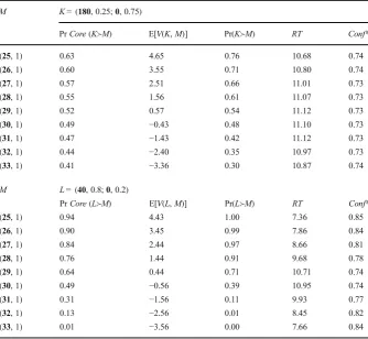
However, violations of SST are a different matter. This can be conveniently illus-trated with an example of the so-called Myers effect (Myers et al. 1965), which constitutes a violation of the independence condition as specified by Tversky and Russo (1969). Table6shows how the probabilities of choosing between each of two lotteries K and L and a series of sure amounts (M) change as the sure sums are progressively increased. The independence condition applied to this case entails that any inequality between Pr(K≻M) and Pr(L≻M) should hold for all values ofM. As Table6shows, this is not the case.
BecauseKhas a wider range of payoffs thanL, PrCore(K≻M) in the top panel of Table 6 changes more slowly than Pr Core(L≻M) in the bottom panel as the sure amountM is increased. For values ofM below 30, PrCore(K≻M) < Pr Core(L≻M), while the opposite is true forMabove 30.
The patterns of RTand Conf* are again closely related to the patterns in choice probabilities. In the top panel, choice probabilities vary less over the range ofMthat we consider, andRTand Conf*also display limited variation. There is more variation in choice probabilities in the bottom panel, matched by more pronounced increases and decreases inRTs and the corresponding opposite patterns inConf*.
3.3.3 Implications for independence and betweenness
[image:15.439.47.389.71.125.2]Many experimental tests of the independence axiom of deterministic EUT have used pairs of lotteries that can be represented in Marschak-Machina (M-M) diagrams such as that shown in Fig.1(Marschak 1950; Machina1982). For any three distinct money
Table 5 Choosing between dominating and dominated lotteries (α= 0.23,β= 1.0, d = 0.1)
A Dominating B Dominated PrCore(A≻B) E[V(A,B)] Pr(A≻B) RT Conf*
payoffs,xh>xm>xl≥0, the vertical axis shows the probability of receivingxhand the
horizontal axis shows the probability of being paidxl, with any residual probability
assigned toxm. Figure1has been drawn forxh= 40,xm= 30 andxl= 0, withA= (30, 1),
B= (40, 0.8;0, 0.2),C= (30, 0.25;0, 0.75),D= (40, 0.2;0, 0.8) andE= (40, 0.2;30, 0.75;0, 0.05).
In any such triangle, deterministic EUT entails that a DM’s preferences can be represent-ed by a set of linear and parallel indifference curves sloping up from south-west to north-east, with the gradient of the lines reflecting her attitude to risk (see Machina1982). The straight and parallel nature of the indifference curves entails that an EU maximiser who choosesA(respectively,B) from pair {A,B} in Fig.1, orA(E) from pair {A,E}, would also chooseC(D) from pair {C,D}. This is an implication of EUT’s independence axiom. In addition, the fact that the indifference curves are linear implies that an EU maximiser choosingA(respectively,B) from pair {A,B}, would also chooseA(E) from pair {A,E} andE(B) from pair {E,B}. This property is known asbetweenness, because the intermediate lotteryEmust lie between the other two in a preference ordering.
[image:16.439.52.387.81.389.2]When applied to the lotteries within an M-M triangle, Becker et al.’s RP form of EUT implies that any pair of lotteries along any straight line of a certain gradient entails
Table 6 ComparingK= (180, 0.25;0, 0.75) andL= (40, 0.8;0, 0.2) against sure amountsMfrom 25 to 33 (α= 0.23,β= 1.0,d= 0.1)
M K =(180, 0.25;0, 0.75)
PrCore(K≻M) E[V(K,M)] Pr(K≻M) RT Conf*
(25, 1) 0.63 4.65 0.76 10.68 0.74
(26, 1) 0.60 3.55 0.71 10.80 0.74
(27, 1) 0.57 2.51 0.66 11.01 0.73
(28, 1) 0.55 1.56 0.61 11.07 0.73
(29, 1) 0.52 0.57 0.54 11.12 0.73
(30, 1) 0.49 −0.43 0.48 11.10 0.73
(31, 1) 0.47 −1.43 0.42 11.12 0.73
(32, 1) 0.44 −2.40 0.35 10.97 0.73
(33, 1) 0.41 −3.36 0.30 10.87 0.74
M L =(40, 0.8;0, 0.2)
PrCore(L≻M) E[V(L,M)] Pr(L≻M) RT Conf*
(25, 1) 0.94 4.43 1.00 7.36 0.85
(26, 1) 0.90 3.45 0.99 7.86 0.84
(27, 1) 0.84 2.44 0.97 8.66 0.81
(28, 1) 0.76 1.44 0.91 9.68 0.78
(29, 1) 0.64 0.44 0.71 10.71 0.74
(30, 1) 0.49 −0.56 0.39 10.95 0.74
(31, 1) 0.31 −1.56 0.11 9.93 0.77
(32, 1) 0.13 −2.56 0.01 8.45 0.82
the same probability of choosing the safer option in the pair (S) over the riskier option (R), with that probability, PrCore(S≻R), reflecting the proportion of the DM’s vNM functions favouringS.12
Experimental work dating back to Allais (1953), Kahneman and Tversky (1979), and many others has shown that these predictions are often systemat-ically violated. While many people are likely to choose the safer option A in pairs such as {A, B} and {A, E}, they tend to choose the riskier option D in pairs such as {C, D} much more frequently, to an extent that the modal choice often reverses. This pattern between pairs {A,B} and {C,D} has come to be known as the common ratio (CR) effect, while significant changes in choice frequencies between {A, E} and {C, D} constitute the common
con-sequence (CC) effect. The betweenness property has also often been found to
be violated, although here the experimental evidence is more variable, some-times showing the intermediate lottery being preferred over each of the two lotteries, other times showing the opposite asymmetry (e.g., Becker et al.
1963b; Coombs and Huang 1976; Bernasconi 1994; see Blavatskyy 2006 for a recent overview).
12
In each pair, the safer option is the one more to the south-west, the riskier the one more to the north-east. So, for example,Ais the safer in {A,B} and {A,E},Cis the safer in {C,D}. Throughout the rest of this section, we will use the convention that the first lottery in any pair {S,R} is the safer and the second is the riskier.
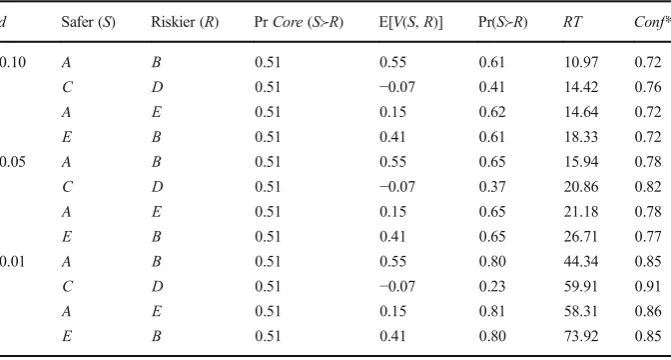
[image:17.439.99.350.50.283.2]The simulations reported in Table7explore the implications of BREUT for the four lottery pairs shown in Fig.1, using three values ofd(0.1, 0.05 and 0.01), and setting α= 0.23, β= 1.0. These parameter values have been chosen to obtain values of Pr Core(S≻R) close to 0.5, allowing us to illustrate how modal preferences can reverse. However, to show that our results are not specific to some special set of parameter values, the online appendix provides three theorems setting out general conditions under which CR, CC and betweenness effects occur.
We start by looking at the E[V(S, R)] column of Table 7. For all pairs except {C, D}, E[V(S, R)] is positive, so we can expect that in each of these pairs the safer option will be chosen with probability 1 with unlimited sampling. The negative value for {C, D} implies that in the limit the riskier option will be chosen with probability 1, in line with both the CR and CC effects. Because of the signs of E[V(S, R)] and the fact that Pr Core(S≻R) = 0.51, Expression6 implies that, with limited sampling, there will be a reversal of modal choice in both the CR and CC scenarios, as we see in all panels of Table 7. As d decreases and the DM samples more, Pr(S≻R) moves further away from 0.5, RTs increase on average and the DM makes her choices with higher confidence.
[image:18.439.52.388.375.555.2]However, whereas BREUT readily produces CR and CC effects, the conditions under which it generates violations of betweenness are much more limited (see Theorem 2 in theonline appendixfor details) and in Table 7 there are no violations of probabilistic betweenness. To the extent that there are substantial systematic viola-tions of betweenness reported in the empirical literature, BREUT does not provide a good account of these.
Table 7 BREUT’s predictions for the independence and betweenness pairs of Fig.1(α= 0.23,β= 1.0)
d Safer (S) Riskier (R) PrCore(S≻R) E[V(S,R)] Pr(S≻R) RT Conf*
0.10 A B 0.51 0.55 0.61 10.97 0.72
C D 0.51 −0.07 0.41 14.42 0.76
A E 0.51 0.15 0.62 14.64 0.72
E B 0.51 0.41 0.61 18.33 0.72
0.05 A B 0.51 0.55 0.65 15.94 0.78
C D 0.51 −0.07 0.37 20.86 0.82
A E 0.51 0.15 0.65 21.18 0.78
E B 0.51 0.41 0.65 26.71 0.77
0.01 A B 0.51 0.55 0.80 44.34 0.85
C D 0.51 −0.07 0.23 59.91 0.91
A E 0.51 0.15 0.81 58.31 0.86
E B 0.51 0.41 0.80 73.92 0.85
A= (30, 1)
B= (40, 0.8;0, 0.2)
C= (30, 0.25;0, 0.75)
D= (40, 0.2;0, 0.8)
4 Discussion and conclusions
In this final section, we consider where BREUT stands in relation to various other models, discuss some of its limitations and identify possible extensions, expand on some broader implications of our findings and offer some conclud-ing remarks.
4.1 BREUT vs. other stochastic models of risky choice
BREUT is quite different in terms of the structure and implications from what is arguably the most standard way of incorporating stochasticity into choice under risk: the Fechnerian version of EUT (e.g., Fechner 1860/1966; Hey and Orme 1994). In Fechnerian models, as applied by economists to EUT, a DM is assumed to have a single vNM utility function which gives a ‘true’ utility difference for one option over another, but her choices are made stochastic by adding some extraneous noise or ‘error’ component. Sometimes this will rein-force her true preference, but sometimes it may work in the opposite direction and—if sufficiently large—may outweigh the true difference, so that on some occasions the DM chooses the truly-less-preferred option. Moreover, the fre-quency with which this occurs may vary from pair to pair, depending on the relationship between the true utility difference and the variance of the error term.
Homoscedastic Fechnerian noise may produce patterns resembling the CR effect, because the utility difference in the {C, D} pair is smaller than in the
{A, B} pair. However, with a zero-median error term, this would not generate
the reversal of modal choice that is so often observed. Moreover, because the EUdifferences for pairs such as {A,E} and {C, D} are of the same magnitude, the model in its simple standard form has no way of producing the CC effect. As shown in Section 3.3, for both the CR and CC effects, BREUT’s implica-tions are clearly different. In addition, the Fechner model would in some cases lead us to expect many more violations of FOSD than are typically observed when dominance is transparent and easy to detect (see Bardsley et al. 2010, Chapter 7, for a discussion).
Some recent refinements of the standard Fechnerian approach have tried to address some of these issues (e.g., Blavatskyy2007,2011; Wilcox2011). However, these more elaborate versions offer no account for the differences in response times and confidence which, as we have seen, are intrinsic to a deliberative process such as the one modelled in BREUT and also consistent with empirical evidence. So, while we do not deny that extraneous noise may have some effect upon the choices we observe, our analysis does not depend on it and all our results are derived as if there were no such additional component.
attention weights and Stage 3 embeds this model in a sequential-sampling framework. At first glance it might seem that Stage 3 DFT is much the same as the model we are proposing, but there are four key differences.
First, in Stage 3 DFT, the specification assumes that the stochastic variability is produced by fluctuations in the probabilities of comparing different pairs of payoffs, rather than fluctuations in the subjective values of those payoffs, which is what BREUT focuses upon. Second, the probabilities are transformed in a way that deviates from EUT. This alone is sufficient to produce non-EU patterns of choice and makes the model unsuitable for exploring the conse-quences of deliberation based strictly upon EU preferences (which is one of the main goals of this paper). Third, the magnitudes being accumulated in Stage 3 DFT are not differences in CEs, but differences between the utilities of the alternative options after they have been weighted by transformed probabilities. Fourth, the sequential-sampling process in DFT takes the form of a Markov process with absorbing thresholds, whereas BREUT uses a stopping rule based on a sequential statistical test. This allows BREUT to make predictions about confidence, which standard DFT (either Stage 3 or the fully-fledged version) is silent about.
After Stage 3, there are various additional stages of elaboration, so that the full (Stage 7) DFT model is considerably more complex than BREUT and involves a larger number of parameters. As a result, this full form of DFT can explain some aspects of decision behaviour that BREUT cannot, such as violations of FOSD for gambles with negatively correlated consequences (see Busemeyer and Townsend1993, p. 447).
4.2 Possible extensions
As stated in the introduction, our objective has not been to reconcile all of the main regularities in risky choice experiments with an EUT core, but rather to explore the implications of embedding a standard deterministic core in a boundedly rational deliberation process. As we indicated, our general modelling approach is not specific to EUT but can be extended to any other core theory that is able to generate CE differences between two options, which makes it potentially very widely applicable.
Humphrey1995) or‘branch-splitting’(Birnbaum2004) effects, which occur when a particular possible outcome of a lottery appears more than once in its description, as well as other so-called paradoxes that have been shown to refute CPT (see Birnbaum
2008).
Our focus in this paper has been upon choices between pairs of risky options, but there have also been many studies reporting anomalies when comparing binary choices with other methods of eliciting preferences. So another direction in which the model-ling of deliberation could usefully be developed concerns the process by which individuals generatematchingorequivalenceresponses. In this context, a task widely used in experiments and surveys is the request to respondents to provide a best estimate of their willingness-to-pay (WTP) or willingness-to-accept (WTA) valuations. In some studies, these are elicited using multiple price lists, which may be regarded as a sequence of pairwise choices. However, asking DMs to work through an ordered list is likely to entail that the choices within the list are not treated independently. Extending sequential sampling models to such tasks would therefore require us to address how this non-independence should be modelled, and what the possible implications might be. In other studies, the elicitation of WTP or WTA is done viaopen-endedquestions, which require the participant to generate a single monetary value as a response. One way of adapting our model to produce responses to this latter procedure might involve sampling utility functions and accumulating the resultingCEs, until an appropriate stopping rule prompts the individual to state a valuation based on the information acquired up to that point. However, there may be other ways of modelling the process behind equivalence judgments,13the exploration of which is a challenge that we leave for future research.
4.3 Concluding remarks
Our analysis shows that deliberative processes may affect the extent to which observed choice probabilities reflect a DM’s underlying distribution of preferences. In BREUT, the DM’s core preferences consist exclusively of vNM utility functions, and in every computation probabilities are applied untransformed, but nevertheless the process of deliberation produces patterns of choice probabilities that systematically depart from those implied by the axioms of EUT.
Our modelling strategy is akin to multiple-selves models (e.g., Elster1987; Alós-Ferrer and Strack2014) in that an individual’s eventual decision may be thought to reflect the aggregate of a sample of certainty equivalents expressed by different inner selves. There is an analogy here with cases in welfare economics where public policy is based on aggregating values over a population of different individuals with heteroge-neous preferences. For example, suppose one were interested in valuing different degrees of risk reduction provided by two alternative interventions using measures of WTP averaged over a sample of individuals. A between-person analogue of our key result (see also Theorem 1 in theonline appendix) would suggest that, even if every person in the sample were a deterministic EU maximiser, there could be a reversal of
13
the aggregate preference over the two interventions simply based on whether the probabilities involved were scaled up or down, even though none of the individual preferences in the population implied such a reversal.
Our results also have implications for experimental investigations of decision making. Recognising the probabilistic nature of choice, one experimental design strategy has involved trying to collect repeated responses to the same decision problems to estimate choice variability. This is a methodology that can lead to complications (e.g., fatigue, boredom, remembering previous decisions, etc.), especially if the number of repetitions is high. However, because response times and confidence judgments are systematically related to choice probabilities, investigators may be able to useRTs and confidence measures in conjunction with fewer repetitions to produce data sets that are less vulnerable to such complications. That implication is not specific to an EUT core,
soRTs may therefore be a useful adjunct to many studies testing a variety of core
theories.
To conclude, the BREUT model set out in this paper can be seen as an illustration of the importance of taking the deliberation process into account when modelling deci-sions, as advocated by Simon many years ago. Allocating theoretical and empirical effort towards exploring the‘production of decisions’ is, we suggest, likely to open fruitful avenues for future research.
Acknowledgements Financial support from the UK Economic and Social Research Council (Grants RES-051-27-0248 and ES/K002201/1), from the Leverhulme Trust‘Value’Programme (RP2012-V-022) and from the Australian Research Council (DP1095681) is gratefully acknowledged.
Open AccessThis article is distributed under the terms of the Creative Commons Attribution 4.0 International License (http://creativecommons.org/licenses/by/4.0/), which permits unrestricted use, distribution, and repro-duction in any medium, provided you give appropriate credit to the original author(s) and the source, provide a link to the Creative Commons license, and indicate if changes were made.
References
Acemoglu, D., & Scott, A. (1994). Consumer confidence and rational expectations: Are agents’beliefs consistent with the theory?Economic Journal, 104(422), 1–19.
Achtziger, A., & Alós-Ferrer, C. (2014). Fast or rational? A response-time study of Bayesian updating.
Management Science, 60(4), 923–938.
Allais, M. (1953). Le comportement de l’homme rationnel devant le risque: Critique des postulates et axiomes de l’ecole Américaine.Econometrica, 21(4), 503–546.
Alós-Ferrer, C., & Strack, F. (2014). From dual processes to multiple selves: Implications for economic behavior.Journal of Economic Psychology, 41, 1–11.
Bardsley, N., Cubitt, R., Loomes, G., Moffatt, P., Starmer, C., & Sugden, R. (2010).Experimental economics: Rethinking the rules. Princeton University Press.
Barsky, R. B., & Sims, E. R. (2012). Information, animal spirits, and the meaning of innovations in consumer choice.American Economic Review, 102(4), 1343–1377.
Baucells, M., & Villasís, A. (2010). Stability of risky preferences and the reflection effect of prospect theory.
Theory and Decision, 68(1-2), 193–211.
Becker, G. M., DeGroot, M. H., & Marschak, J. (1963a). Stochastic models of choice behavior.Behavioral Science, 8, 41–55.
Bernasconi, M. (1994). Nonlinear preferences and two-stage lotteries: Theories and evidence.Economic Journal, 104(422), 54–70.
Binmore, K. (2009). Interpersonal comparison of utility. In D. Ross & H. Kincaid (Eds.),The Oxford handbook of philosophy of economics(pp. 540–559). New York: Oxford University Press.
Birnbaum, M. H. (2004). Tests of rank-dependent utility and cumulative prospect theory in gambles represented by natural frequencies: Effects of format, event framing, and branch splitting.
Organizational Behavior and Human Decision Processes, 95(1), 40–65.
Birnbaum, M. H. (2008). New paradoxes of risky decision making.Psychological Review, 115(2), 463–501. Birnbaum, M. H., & Jou, J. (1990). A theory of comparative response times and‘difference’judgments.
Cognitive Psychology, 22(2), 184–210.
Birnbaum, M. H., & Navarrete, J. B. (1998). Testing descriptive utility theories: Violations of stochastic dominance and cumulative independence.Journal of Risk and Uncertainty, 17(1), 49–79.
Blavatskyy, P. R. (2006). Violations of betweenness or random errors?Economics Letters, 91(1), 34–38. Blavatskyy, P. R. (2007). Stochastic expected utility theory.Journal of Risk and Uncertainty, 34(3), 259–286. Blavatskyy, P. R. (2011). A model of probabilistic choice satisfying first-order stochastic dominance.
Management Science, 57(3), 542–548.
Brandstätter, E., Gigerenzer, G., & Hertwig, R. (2006). The priority heuristic: Making choices without trade-offs.Psychological Review, 113(2), 409–432.
Busemeyer, J. R., & Townsend, J. T. (1993). Decision field theory: A dynamic-cognitive approach to decision making in an uncertain environment.Psychological Review, 100(3), 432–459.
Butler, D., & Loomes, G. (1988). Decision difficulty and imprecise preferences.Acta Psychologica, 68(1-3), 183–196.
Butler, D., Isoni, A., Loomes, G., & Tsutsui, K. (2014a). Beyond choice: Investigating the sensitivity and validity of strength of preference measures.Experimental Economics, 17(4), 537–563.
Butler, D., Isoni, A., Loomes, G., & Navarro-Martinez, D. (2014b). On the measurement of strength of preference in units of money.Economic Record, 90, 1–15.
Cerreia-Vioglio, S., Dillenberger, D., & Ortoleva, P. (2015). Cautious expected utility and the certainty effect.
Econometrica, 83(2), 693–728.
Coombs, C., & Huang, L. (1976). Tests of the betweenness property of expected utility.Journal of Mathematical Psychology, 13(3), 323–337.
Dominitz, J., & Manski, C. F. (2004). How should we measure consumer confidence?Journal of Economic Perspectives, 18(2), 51–66.
Elster, J. (1987).The multiple self. Cambridge: Cambridge University Press.
Fechner, G. T. (1860/1966).Elements of psychophisic. New York: Holt, Rinehart and Winston. Gigerenzer, G., & Selten, R. (2001).Bounded rationality: The adaptive toolbox. MIT Press.
Gilboa, I., & Schmeidler, D. (1995). Case-based decision theory.Quarterly Journal of Economics, 110(3), 605–639.
Gold, J. I., & Shadlen, M. N. (2007). The neural basis of decision making.Annual Review of Neuroscience, 30(1), 535–574.
Griffin, D., & Tversky, A. (1992). The weighing of evidence and the determinants of confidence.Cognitive Psychology, 24(3), 411–435.
Hammond, P. (1993). Interpersonal comparisons of utility: Why and how they are and should be made. In J. Elster & J. Roemer (Eds.),Interpersonal comparisons of well-being. London: Cambridge University Press. Hausmann, D., & Läge, D. (2008). Sequential evidence accumulation in decision making: The individual desired level of confidence can explain the extent of information acquisition.Judgment and Decision making, 3(3), 229–243.
Hey, J. D., & Orme, C. (1994). Investigating generalizations of expected utility theory using experimental data.Econometrica, 62(6), 1291–1326.
Humphrey, S. J. (1995). Regret aversion or event-splitting effects? More evidence under risk and uncertainty.
Journal of Risk and Uncertainty, 11(3), 263–274.
Jamieson, D. G., & Petrusic, W. M. (1977). Preference and time to choose.Organizational Behavior and Human Performance, 19(1), 56–67.
Johnson, J. G., & Busemeyer, J. R. (2005). A dynamic, computational model of preference reversal phenomena.Psychological Review, 112(4), 841–861.
Johnson, E. J., Häubl, G., & Keinan, A. (2007). Aspects of endowment: A query theory of value construction.
Journal of Experimental Psychology: Learning, Memory, and Cognition, 33, 461–474.
Koehler, D. J. (1991). Explanation, imagination, and confidence in judgment.Psychological Bulletin, 110(3), 499–519.
Koriat, A., Lichtenstein, S., & Fischhoff, B. (1980). Reasons for confidence.Journal of Experimental Psychology: Human Learning and Memory, 6(2), 107–118.
Loomes, G., Moffatt, P. G., & Sugden, R. (2002). A microeconometric test of alternative theories of risky choice.Journal of Risk and Uncertainty, 24(2), 103–130.
Luce, R. D. (1992). A theory of certainty equivalents for uncertain alternatives.Journal of Behavioral Decision Making, 5(3), 201–216.
Luce, R. D., & Suppes, P. (1965). Preferences, utility, and subjective probability. In R. D. Luce et al. (Eds.),
Handbook of mathematical psychology(Vol. 3). New York: John Wiley.
Luce, R. D., Mellers, B., & Chang, S. J. (1993). Is choice the correct primitive? On using certainty equivalents and reference levels to predict choices among gambles.Journal of Risk and Uncertainty, 6(2), 115–143. Ludvigson, S. C. (2004). Consumer confidence and consumer spending.Journal of Economic Perspectives,
18(2), 29–50.
Machina, M. (1982).BExpected utility^analysis without the independence axiom.Econometrica, 50(2), 277–323. Marschak, J. (1950). Rational behavior, uncertain prospects, and measurable utility.Econometrica, 18(2),
111–141.
Moffatt, P. (2005). Stochastic choice and the allocation of cognitive effort.Experimental Economics, 8(4), 369–388.
Moffatt, P., & Peters, S. (2001). Testing for the presence of a tremble in economic experiments.Experimental Economics, 4(3), 221–228.
Mosteller, F., & Nogee, P. (1951). An experimental measurement of utility.Journal of Political Economy, 59(5), 371–404.
Myers, J., Suydam, M., & Gambino, B. (1965). Contingent gains and losses in a risk-taking situation.Journal of Mathematical Psychology, 2(2), 363–370.
Otter, T., Johnson, J., Rieskamp, J., Allenby, G. M., Brazell, J. D., Diedrich, A., Hutchinson, J. W., MacEachern, S., Ruan, S., & Townsend, J. (2008). Sequential sampling models of choice: Some recent advances.Marketing Letters, 19(3-4), 255–267.
Payne, J. W., Bettman, J. R., & Johnson, E. J. (1993).The adaptive decision maker. Cambridge: Cambridge University Press.
Petrusic, W. M., & Jamieson, D. G. (1978). Relation between probability of preferential choice and time to choose changes with practice. Journal of Experimental Psychology: Human Perception and Performance, 4, 471–482.
Pleskac, T. J., & Busemeyer, J. R. (2010). Two-stage dynamic signal detection: A theory of choice, decision time, and confidence.Psychological Review, 117(3), 864–901.
Ratcliff, R., & Smith, P. L. (2004). A comparison of sequential sampling models for two-choice reaction time.
Psychological Review, 111(2), 333–367.
Rieskamp, J., Busemeyer, J., & Mellers, B. (2006). Extending the bounds of rationality: Evidence and theories of preferential choice.Journal of Economic Literature, 44(3), 631–661.
Rubinstein, A. (1988). Similarity and decision making under risk: Is there a utility theory resolution to the Allais paradox?Journal of Economic Theory, 46(1), 145–153.
Rubinstein, A. (2007). Instinctive and cognitive reasoning: A study of response times.The Economic Journal, 117(523), 1243–1259.
Rubinstein, A. (2013). Response time and decision making: An experimental study.Judgment and Decision Making, 8(5), 540–551.
Shiryaev, A. N. (1978).Optimal stopping rules. Berlin Heidelberg: Springer-Verlag.
Sieck, W., & Yates, J. F. (1997). Exposition effects on decision making: Choice and confidence in choice.
Organizational Behavior and Human Decision Processes, 70(3), 207–219.
Simon, H. A. (1978). Rationality as process and as product of thought.American Economic Review, Papers and Proceedings, 68(2), 1–16.
Spiliopoulos, L., & Ortmann, A. (2016). The BCD of response time analysis in experimental economics. Available at SSRN:http://ssrn.com/abstract=2401325.
Starmer, C. (2000). Developments in non-expected utility theory: The hunt for a descriptive theory of choice under risk.Journal of Economic Literature, 38(2), 332–382.
Starmer, C., & Sugden, R. (1993). Testing for juxtaposition and event-splitting effects.Journal of Risk and Uncertainty, 6(3), 235–254.
Stewart, N., Chater, N., & Brown, G. D. A. (2006). Decision by sampling.Cognitive Psychology, 53(1), 1–26. Stewart, N., Reimers, S., & Harris, A. J. L. (2015). On the origin of utility, weighting, and discounting functions:
Stigler, G. J. (1961). The economics of information.Journal of Political Economy, 69(3), 213–225. Tversky, A. (1972). Elimination by aspects: A theory of choice.Psychological Review, 79(4), 281–299. Tversky, A., & Russo, J. E. (1969). Substitutability and similarity in binary choices.Journal of Mathematical
Psychology, 6(1), 1–12.
Tversky, A., & Kahneman, D. (1992). Advances in prospect theory: Cumulative representation of uncertainty.
Journal of Risk and uncertainty, 5(4), 297–323.
Tyebjee, T. (1979). Response time, conflict and involvement in brand choice.Journal of Consumer Research, 6(3), 295–304.
Wilcox, N. T. (1993). Lottery choice: Incentives, complexity and decision time.The Economic Journal, 103(421), 1397–1417.