Progressive preference articulation for decision making in multi objective optimisation problems

Progressive Preference Articulation for Decision

Making in Multi-Objective Optimisation Problems

Shahin Rostamia,1, Ferrante Nerib,2and Michael G. Epitropakisc

a_{Faculty of Science and Technology, Bournemouth University, Bournemouth, United Kingdom}

b_{School of Computer Science and Informatics, De Montfort University, Leicester, United Kingdom}

c_{Data Science Institute, Department of Management Science, Lancaster University Management School,} Lancaster University, Lancaster, United Kingdom

Abstract.

This paper proposes a novel algorithm for addressing multi-objective optimisation problems, by employing aprogressivepreference articu-lation approach to decision making. This enables the interactive incorporation of problem knowledge and decision maker preferences during the optimisation process. A novel progressive preference articulation mechanism, derived from a statistical technique, is herein proposed and implemented within a multi-objective framework based on evolution strategy search and hypervolume indicator selection. The proposed algo-rithm is named the Weighted Z-score Covariance Matrix Adaptation Pareto Archived Evolution Strategy with Hypervolume-sorted Adaptive Grid Algorithm (WZ-HAGA).

WZ-HAGA is based on a framework that makes use of evolution strategy logic with covariance matrix adaptation to perturb the solutions, and a hypervolume indicator driven algorithm to select successful solutions for the subsequent generation. In order to guide the search towards interesting regions, a preference articulation procedure composed of four phases and based on the weighted z-score approach is employed. The latter procedure cascades into the hypervolume driven algorithm to perform the selection of the solutions at each generation.

Numerical results against five modern algorithms representing the state-of-the-art in multi-objective optimisation demonstrate that the pro-posed WZ-HAGA outperforms its competitors in terms of both the hypervolume indicator and pertinence to the regions of interest.

Keywords.multi-objective optimisation, many-objective optimisation, evolution strategy, selection mechanisms, preference articulation

1. Introduction

Multi-objective optimisation is the search for solutions that display the best performance in the presence of multiple conflicting objectives, see e.g. [75,61,35]

With the exception of a few trivial problems, these types of problem often do not have a single optimal so-lution. Instead, a (finite or infinite) set of solutions will offer the same level of optimality whereby an increase in the performance of one objective will result in the decrease of another [16,45,38]. Two solutions of this description are said tonot dominate each other and

2_{Corresponding Author: Faculty of Science and Technology,}

Bournemouth University, Fern Barrow, BH12 5BB, Bournemouth, United Kingdom, E-mail: [email protected].

2_{Corresponding Author: School of Computer Science and}

Engi-neering, De Montfort University, The Gateway House, LE1 9BH, Leicester, United Kingdom, E-mail: [email protected].

the set of solutions which do not dominate each other is referred to as a non-dominated front. Conversely, when a solution outperforms another solution in re-spect to all the considered objectives, the solution can be described asdominatingthe other. The theoretical set containing all the solutions which cannot be dom-inated is referred to as thePareto set,Pareto front, or simply thePareto.

im-plementation of the design suggested by the algorithm, see e.g.[1,56,11].

For these reasons, multi-objective problems can be considered to require a two stage approach: during the first stage an approximation of the Pareto is iden-tified, see [48,36], and during the second stage the de-cision regarding which solution must be selected from the approximation set, is made. The second stage is fo-cussed onDecision Makingand the criteria which ar-ticulate the biases of the decision making process are referred to as Decision Maker (DM) preferences.

When solving real-world multi-objective prob-lems, the ideal optimisation algorithm is one which converges to an approximation set consisting of non-dominated solutions which are within the DM’s Re-gion of Interest (ROI). The ideal algorithm would ig-nore solutions which are not of interest to the DM, even if they are non-dominated, and instead focus on areas of the objective space which are of interest to the DM. The integration of DM preferences into the algorithm can be interpreted as a simplification of the complexity of the problem since, effectively, it corre-sponds to a reduction of the search space, similar to what happens in various fields of engineering. This logic is commonly applied in finite element methods, see [60].

Other examples in computational mechanics and engineering are reported in [12] for structural damage detection, in [67] for selecting the most suitable type of foundation, and in [6] for non-linear system param-eter identification and a reduction of the mathematical model. An application to seismic retrofit design with algorithmic distribution over multiple cores and com-puters has been proposed in [39].

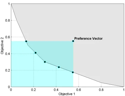
The formalisation of the concept of interest is connected to the concept of thepertinence of an ap-proximation set illustrated in Fig. 1 and 2. An approx-imation set offers good pertinence if most of its solu-tions belong to the ROI, see Fig. 1, and is composed of a small set of solutions. Subsequently, the DM is not overwhelmed with a large set of global trade-off solu-tions (illustrated in Fig. 2) when using expert knowl-edge to select their desired solution [24].

Furthermore, when a ROI is specified through the definition of preferences (i.e. the importance or goal of each objective with respect to the others is defined), this piece of information can be integrated within the

Figure 1. An approximation set containing five solutions with ideal pertinence, i.e., all Pareto Efficient solutions are within the rectangle defined by the DM’s preference vector.

optimisation algorithm to guide the search and pursue only pertinent solutions. An algorithm modified in this way is able to exploit the information about prefer-ences during the search to discard trade-off solutions which do not fall within the desired region, and to pressure the search towards the region by influencing the algorithm’s selection operator, see [37]. This ad-ditional preference information ultimately reduces the area of feasible solutions within the objective space, thus reducing the computational effort needed to pro-duce a diverse set of pertinent solutions.

1.1. Progressive Preference Articulation: A brief review

The action of the DM can occur in three moments of the optimisation, coinciding with the following ap-proaches.

• A priori, in which preferences are defined be-fore the search, see [68,70].

• A posteriori, in which the DM selects a

solu-tion after complesolu-tion of a search, see [41,76, 13].

• Progressive, involving interaction with the DM during execution of the search, see [26].

un-Figure 2. An approximation set containing seven solutions where four of them exhibit undesirable pertinence, i.e., there are four Pareto Efficient solutions that are not within the hyper-rectangle de-fined by the DM’s preference vector.

interesting areas of the search space could be unnec-essarily explored and some areas of the search space which potentially deserve attention could be missed, [70].

Whilst thea posterioriapproach avoids this dis-advantage by only considering preference information after the optimisation process, it does not offer any advantages throughout the optimisation process and causes an extremely high computational cost in com-parison.

The progressive approach, which is the focus of this article, potentially enables the DM to alter their preferences during the optimisation process and incor-porate knowledge that only becomes available during the search [14], such as the exact nature of trade-offs between objectives.

The technique of progressively incorporating preferences into the multi-objective optimisation pro-cess is referred to as progressive preference articu-lation, see [14] and [49]. A comparative analysis of the various approaches of preference articulation is re-ported in [2] and in the talk [25].

One of the first schemes for progressive prefer-ence articulation in population-based meta-heuristics for multi-objective optimisation was introduced by [27], and extended the Pareto-based ranking scheme used in the Multiple Objective Genetic Algorithm (MOGA) [26] to allow preferences to be expressed

throughout the execution of a population-based algo-rithm. Subsequently, in [7] preferences are integrated in the algorithm simplistically by means of linear max-imum and minmax-imum trade-off functions. In [8] two methods based on a biased crowding technique are presented and compared.

The R-Non-dominated Sorted Genetic Algorithm II (R-NSGA-II) presented in [18], combines a pref-erence based strategy with an evolutionary multi-objective algorithm, in order to demonstrate how a preferred set of solutions near a number of reference-points can be found simultaneously. In [17] the ε

Multi Objective Evolutionary Algorithm (ε-MOEA)

has been introduced. The latter algorithm also inte-grated the DM to control the achievable accuracy of non-dominated solutions. A self-adaptive version of theεlogic is proposed in [62]

To overcome the shortcomings of not having preference information in the selection process of the Indicator-Based Evolutionary Algorithm (IBEA) [77], the Preference-Based Evolutionary Algorithm (PBEA) was introduced in [65]. In [3] an approach that integrates the DM’s preferences into an estimation of the dominated portion of the objective space (hy-pervolume) is presented. In [9] two ranking schemes integrating the preference articulation have been pro-posed. However, the calculation of the hypervolume indicator presents the drawback that it depends expo-nentially on the number of objectives and therefore becomes infeasible for multi-objective problems with many objectives, see [4].

To effectively incorporate the DM’s preferences in well-known multi-objective evolutionary algorithms, new variants of Pareto dominance relations have been recently proposed. Popular examples are the r -dominance [55] andg-dominance relations [46]. The r-dominance biases the search procedure towards the ROI by using the weighted Euclidean distance intro-duced in [18] while using a dominance based criterion to select the population for the following generation. The g-dominance biases the search towards the ROI by applying a penalisation criterion to those solutions that are outside (and far away) from the ROI. In [74], the use of a weight vector is made to detect solutions around it (in the objective space).

op-timisation algorithm, also aims to allow the incorpo-ration of preference information. The incorpoincorpo-ration of preferences is implemented by simply providing dif-ferent weightings or “reference-points” when initialis-ing the algorithm. However, there is no way for a de-cision maker to provide a preference vector or “goal”, they must instead design a structure of weights which are distributed to reflect the preferences. Although the NSGA-III implementation appears to have several am-biguities, see [33], the algorithm is an important con-tribution to the field.

Another fundamental and modern algorithm which makes use of structured weights, and enhances its con-vergence performance by decomposing the domain, is the θ-Dominance based Evolutionary Algorithm

(θ-DEA) [71]. The latter algorithm has demonstrated very high performance on a number of diverse prob-lems and is currently one of the state-of-the-art algo-rithms in the field.

Preference articulation is applied to several engi-neering many-objective problems in [43]. Reference-points, similar to those employed in NSGA-III, are also used in [54]. The functioning of the latter is based on the use of an achievement scalarising function and the classification of solutions into several fronts.

In [22] an interactive algorithm based on R-NSGA-II is proposed, and in [23] R-R-NSGA-II is mod-ified by integrating a stochastic local search in a memetic fashion, see [47], [10], [32], and [72].

Since the objectives of the problem are estab-lisheda prioribut their importance is adjusted on-line by human experts, progressive preference articulation can be interpreted as an interactive design method and can be linked to a large and interesting portion of the literature. In [44], a system that interactively collects data and predicts the posture of workers for medical purposes has been proposed. An interactive fuzzy multi-objective algorithm for engineering prob-lems has been proposed in [29]. Interactive design with reference to steel structure design is achieved by integrating fuzzy logic into the constraint handling in [58,57]. In order to handle large steel structures the al-gorithm proposed in [59] expands the previous the two studies above in a parallel fashion.

This paper proposes a novel progressive prefer-ence articulation mechanism for multi-objective op-timisation problems. Furthermore, this mechanism is

incorporated into an optimisation framework recently proposed in the literature, namely the Covariance Matrix Adaptation Pareto Archived Evolution Strat-egy with Hypervolume-sorted Adaptive Grid Algo-rithm (CMA-PAES-HAGA), see [50]. The resulting algorithm has been thoroughly tested and compared against modern algorithms which implicitly and ex-plicitly incorporate preference articulation.

The remainder of the article is arranged in the fol-lowing order: Section 2 describes all the components of the proposed algorithm. Section 3 describes the ex-perimental setup, and presents the results of the mul-tiple comparison between the proposed algorithm and five other many-objective optimisation algorithms, all of which represent the state-of-the-art in the field. Sec-tion 4 concludes the study and offers research direc-tions for future work.

2. Weighted Z-score Covariance Matrix

Adaptation Pareto Archived Evolution Strategy with Hypervolume-sorted Adaptive Grid Algorithm

This section describes the proposed algorithm, named the Weighted Z-score Covariance Matrix Adaptation Pareto Archived Evolution Strategy with Hypervolume-sorted Adaptive Grid Algorithm. The proposed algo-rithm will be referred to as WZ-HAGA hereafter for brevity.

The proposed approach consists of two significant parts, these are:

• the incorporation of DM preferences within the search logic to drive the search towards the ROI: the Weighted Z-score (WZ) preference ar-ticulation,

• the external framework for multi-objective op-timisation that hosts the progressive incorpora-tion of the WZ preference articulaincorpora-tion: CMA-PAES-HAGA.

al-gorithm is then outlined in Section 2.4. Finally, with the purpose of highlighting the differences between a prioriandprogressiveincorporation of DM prefer-ences, Section 2.5 contrasts both the implementations.

2.1. Background – Notation

This section briefly presents some essential notation and background information that is required to clearly define the proposed progressive preference articula-tion approach.

Without loss of generality, let us define a general multi-objective optimisation problem (MOP) withM objective functions(F={f1,f2, . . . ,fM}):D→RM), that are to be optimised (minimised or maximised); in its general form it can be defined as follows:

Optimise fm(x), m=1,2, . . . ,M; subject to gj(x)≥0, j=1,2, . . . ,J;

hk(x) =0, k=1,2, . . . ,K; xLB_i ≤xi≤xU Bi ,i=1,2, . . . ,D,

(1)

wherex is a solution vector of D decision variables:

x=hx1,x2, . . . ,xDi>,in which each decision variable is confined by a lower (xLB_i ) and an upper (xUB_i ) bound. Such bounds constitute the decision spaceD of the problem. Inequality (gj(x)) and equality (hk(x)) con-straints can be also imposed to restrict the feasible de-cision space of the given problem. The corresponding set of all possible values that the solutions can take within the feasible decision space constitutes the ob-jective space (OM_⊆

RM).

Given a population-based search algorithm, let us also define a populationXof N potential solution vec-tors X=hx1,x2, . . . ,xNi, i.e.,X is a matrix of N by D entries. As such, xi j denotes the j-th element of the solution vector xi. LetY be an M by N matrix

that represents the objective values of the population X,Y =F(X) =hy1,y2, . . . ,yNi, whereyi =hf1(xi), f2(xi), . . . ,fM(xi)i>.Clearly,yi j denotes the j-th ob-jective value of the solution vectorxi. Let also P= hρ1,ρ2, . . . ,ρMito be a preference vector in the objec-tive space that can be defined by the DM.

In this paper we work within an evolution strategy framework. In accordance with the notation used in the field, the parent population size is indicated withµ

while the offspring population size is indicated withλ, see [50]. As shown in the following subsections, theµ

parent solutions generateλoffspring solutions at each

generation, andµsolutions must then be selected from

the N=µ+λ solutions in X.

2.2. External Optimisation Framework

The external framework embedding the WZ prefer-ence articulation operator is the CMA-PAES-HAGA framework proposed in [50]. This algorithmic frame-work uses the search exploration of the Pareto Adap-tive Evolution Strategy (PAES) using a random per-turbation aided by a Gaussian distribution, see [41], combined with Covariance Matrix Adaptation logic, see [28]. The selection mechanism is based on the hypervolume indicator by means of a fast algorithm, see [50,51] and is referred to as the HAGA selection scheme. The latter is a selection algorithm that maps a grid within the objective space and uses the grid lo-cation of the solutions to estimate the hypervolume in-dicator, i.e. the portion of objective space dominated by the approximation set. The estimation technique in [51] is almost as reliable as the hypervolume indicator, but is much faster in terms of calculation time.

Although all the implementation details about this framework are reported in [50], a simplified pseudo-code listing describing the working principles of CMA-PAES-HAGA is displayed in Algorithm 1 for the sake of clarity.

2.3. Incorporating Decision Maker Preferences into the Search Logic: Weighted Z-score preference articulation

Weighted Z-score (WZ) preference articulation is a re-cently proposed method for incorporating DM prefer-ences, based around the use of z-scores (or standard scores) from Statistics [52,53]. The purpose of the fol-lowing procedure is to assign a score to each candi-date solution which describes the position of the point (in the objective space) with respect to the ROI. These scores are then used during the selection.

Let us consider a populationXcomposed on N=

µ+λ individuals/vectors. A generic nth individual

is a vector xn associated with its M objectivesyn=

Algorithm 1CMA-PAES-HAGA execution cycle 1: Initialise parent populationXcomposed ofµ

par-ent solutions and corresponding objective values Y

2: whiletermination criteria not metdo

3: forall theλ solutions of the offspring popula-tiondo

4: Generate an offspring solution by variation operators, i.e. perturbation by means of Gaussian distribution and covariance matrix, as in [41,28] 5: Check that the solution is within the

bounds of the decision space. If it is outside the decision space, the solution is saturated to the closest bound.

6: Calculate the objective values of the solu-tion

7: end for

8: Perform the HAGA selection to compose the new parent population (selectµsolutions) by hy-pervolume estimation as in [50,51]

9: Update the covariance matrix adaptive param-eters as in [28]

10: end while

Furthermore, as mentioned above, P=hρ1,ρ2, . . . ,ρMi is a preference vector in the objective space defined by the DM. Let us indicate withρmthe generic goal value set by the DM on themthobjective.

With these values, a matrix, namely the Z-matrix, is calculated. Each matrix elementzmnrepresents the z-score for thenth candidate solution with respect to themthobjective and is calculated according to the fol-lowing equation:

zmn=

(ymn−ρm) r

∑N_j=1(ym j−ρm)2

N

. (2)

Eachzmnvalue will take a positive value when it is outside the ROI, and a negative value when within the ROI.

With the ymn objective function values of theY matrix and the valuesρm of the preference vector P, another matrix, indicated with S is calculated. Each entrysmnofSis calculated as:

smn= (

1, ifymn≤ρm

0, otherwise. (3)

The entries of theS matrix are then used to re-solve whether or not each individual of the population X belongs to the ROI.

Thus, the generic individualxnis associated to the

followingφnvalue:

φn=

M

∏

smn. (4)

Furthermore, φn=1 if the candidate solutionxn

belongs to the ROI andφn=0 otherwise. Subsequently the scalarψis calculated:

ψ=

N

∑

φn. (5)

The scalarψ refers to the number of solutionsxn in the population that have satisfied the preference vec-tor P, i.e. the number of solutions inside the ROI.

Let us indicate with ψthresh the required number of solutions that satisfy the preference vector. This pa-rameter is then used in a two-phase mechanism which aims at guiding the search towards the ROI. The two phases, namely the W-phase and the Z-phase, consist of the following steps.

When the number of solutions within the ROI has satisfied the threshold (ψ≥ψthresh) theZ-phasetakes effect. This phase uses eq. (2) to calculate theZmatrix and then eq. (6) to aggregate the scores into the scalar vn:

vn=∑ M m=1zmn

M . (6)

Thus, each candidate solutionxnis associated a score

vn.

However, ifψ<ψthreshthen theW-phaseof the WZ preference articulation operator takes effect. In or-der to explain the set of operations which occur during the W-phase, let us consider the generic objective fm. Let us indicate withωmthe following scalar:

ωm=

N

∑

It can be observed thatωm refers to the number of solutions in the population that have satisfied the correspondingρm. In the same way, anωmvalue can be calculated for each objective function and a vector Ω=hω1,ω2, . . . ,ωMiis then defined.

With the entries ofω calculated, another matrix, indicated with E, is calculated.

At first, the normalised values (between 0 and 1) z∗_mnandω_m∗ofzmnandωm, respectively, are calculated:

z∗_mn= |zmn| −min(|zm|) max(|zm|)−min(|zm|)

, (8)

where|zmn|is the absolute value ofzmnand|zm|is the mthcolumn vector of theZmatrix where for each ele-ment the absolute value has been calculated, and

ω_m∗=ωm

N . (9)

The entriesεmnof the matrixEare then calculated as:

εmn=

(

z∗_mn 1− 1 M

if ωm−min(Ω)

max(Ω)−min(Ω)=0,

z∗_mn otherwise. (10)

The purpose of eq. (10) is to ensure that those objec-tives that least satisfy the DM requirements must be corrected by the weighting factor 1− 1

M

.

The final scorewnof a single solution is the ag-gregation of the correspondingεmnentries:

wn=

∑Mm=1εmn

M . (11)

Thus, each candidate solutionxn is associated a

scorewn.

This method attempts, when many solutions are outside the ROI, to move the search towards the pro-duction of solutions that are close in proximity to the ROI and within it, but does not attempt to minimise the solutions beyond the edges of the ROI.

For the sake of clarity, the working principles of the weighted Z-score preference articulation selection are highlighted in Algorithm 2.

Algorithm 2Weighted Z-score preference articulation 1: Input the X population (whose candidate solutions arexn), the objectives Y, the preference vector P, and the thresholdφthresh.

2: forall the candidate solutionsn=1 : Ndo

3: forall the objectivesm=1 : Mdo

4: Calculate the Z matrix elementzmn, eq. (2) 5: Calculate the S matrix elementsmn, eq.(3) 6: end for

7: end for

8: forall the candidate solutionn=1 :Ndo

9: Calculateφn, eq. (4) 10: end for

11: Calculateψ, eq. (5)

12: ifψ≥ψthreshthen . Z-phase

13: forall the objectivesm=1 : Mdo

14: Calculatevn, eq. (6), and assign it toxn

15: end for

16: else ifψ<ψthreshthen . W-phase 17: forall the objectivesm=1 : Mdo

18: Calculateωmof the vectorΩ, eq. (7) 19: end for

20: forall the candidate solutionsn=1 : Ndo

21: forall the objectivesm=1 : Mdo

22: Normalisezmnandωm

23: Calculate the elementεmn, eq. (10) 24: end for

25: end for

26: forall the candidate solutionsn=1 : Ndo

27: Calculatewn, eq. (11), and assign it toxn

28: end for

29: end if

2.4. Selection mechanism of WZ-HAGA

Let us consider a population X composed ofµ+λ=N candidate solutions.

The selection of the WZ-HAGA, see Algorithm 1, operates in one of the following four phases to select theµcandidate solutions composing the parent

popu-lation for the following generation.

Phase 1is active when there are no solutions in the current approximation set which are within the ROI, i.e. ψ=0. This phase uses the W-phase of the

Phase 2is active whilst the number of solutions in the ROI is below the thresholdψthreshintroduced in Section 2.3, i.e. 0<ψ <ψthresh. This phase contin-ues to use the W-phase of WZ algorithm described in Section 2.3 whilst explicitly retaining solutions in the archive that are within the DM’s expressed ROI. Then the solutions inside the ROI and those with highestwn score are selected.

Phase 3is active when the number of solutions in the ROI equal or exceedψthresh, i.e.ψthresh≤ψ<µ. This phase uses the Z-phase of Section 2.3 whilst re-taining solutions in the current approximation set that are within the DM’s expressed ROI. This phase aims to populate the current archive entirely with solutions that are within the current ROI.

Phase 4is active when among theµ+λ=N

can-didate solutions, at leastµof them are within the ROI,

i.e.ψ ≥µ. All solutions that are not within the ROI

are automatically discarded. The remaining solutions (which are in the ROI) are subjected to the hypervol-ume based CMA-PAES-HAGA selection mechanism (HAGA selection), refer to [50,51].

By using these four phases, the optimisation pro-cess is able to quickly get as close as possible to the DM’s expressed ROI, produce solutions within it, have a parent population with solutions only within that ROI, and then converge further into that ROI with a diverse approximation set. Finally, it is possible to regress from later phases to earlier ones depending on the optimisation context, i.e. if the DM alters their preferences during the optimisation process.

2.5. A Priori and Progressive Preference Articulation

Although this article proposes aprogressiveapproach to preference articulation, WZ-HAGA can be imple-mented either with onlya prioriarticulation of pref-erences, or Progressive Preference Articulation herein referred to as WZ-HAGA (PPA) in this section.

The pseudocode listing for the execution cycle of WZ-HAGA (PPA) has been illustrated in Algorithm 3. The pseudocode highlights the mechanism for han-dling solutions that are inside or outside the ROI by means of the phases described in Section 2.4. In itsa prioriversion of the same algorithm, the input of the DM is established prior to the beginning of the algo-rithm execution and remains static throughout the

en-tire optimisation process. In the PPA version described in Algorithm 3, the optimisation process can be con-figured to prompt the DM for a new preference point at configured intervals (e.g. every 100 generations). At these intervals, HAGA is used to reduce the ap-proximation set for the DM, such that they are able to use new information about the objective space and the emerging trade-offs, to make an informed decision on a new set of preferences. The optimisation process then continues without discarding the existing solu-tions.

3. Numerical Results

This section presents the results of this study. The ex-perimental setup is described, and then the results are presented and discussed. Finally, a real-world appli-cation of the proposed WZ-HAGA is demonstrated within the field of engineering control systems design.

3.1. Experimental Setup

The performance of the proposed algorithm has been evaluated and compared against five state-of-the-art multi-objective optimisation algorithms. The algo-rithms included in this study are:

1. WZ-HAGA: with reference to Subsection 2.4 the parameterψthresh=M where M is the num-ber of solutions needed within the ROI for the Z-phase to take effect; with reference to the ex-ternal framework in Subsection 2.2, the num-ber of grid-divisions isδ =3 as suggested in [51];

2. NSGA-III: with reference to [15] crossover probability 0.9, crossover distribution index 30, mutation distribution index 20;

3. θ-DEA: with reference to [71],θ=5,div1=

3,div2=0, crossover probability 1, crossover distribution index 30, mutation probability 1, mutation distribution index 20.

Algorithm 3Progressive preference articulation and selection within WZ-HAGA

1: Input the initial preference vector P.

2: Initialise parent population in the search space and the corresponding vectors of objective values 3: whiletermination criteria not metdo

4: (Optional) Input the updated preferences ex-pressed by the DM and consequent modification of vector P and thus the ROI. .Progressive Preference Articulation

5: forall the offspring solutionsλdo

6: Apply CMA-PAES variation operators to the parent population in order to generate an off-spring solution

7: Calculate and store the objective function values

8: Check the objective values and whether or not the solution is within the ROI

9: Merge parent and offspring population into X

10: end for

11: Calculate the numberψof solutions within the

ROI by eq. (5) and perform the selection of the new parent population (µcandidate solutions): . Selection mechanism

12: if ψ=0then

13: Phase 1: Use thewnscore values to select the bestµsolutions (W-phase)

14: else if 0<ψ<ψthreshthen

15: Phase 2: Save theψ solutions inside the ROI and use thewnscore values to select the best remainingµ−ψ solutions (W-phase)

16: else if ψthresh≤ψ<µthen

17: Phase 3: Save theψ solutions inside the ROI and use thevnscore values to select the best remainingµ−ψ solutions (Z-phase)

18: else if ψ≥µthen

19: Phase 4: Discard the solutions outside the ROI and apply HAGA selection scheme [50,51] to selectµcandidate solutions

20: end if

21: end while

5. r-NSGA-II: with reference to [55,66] crossover probability 1, crossover distribution index 30, mutation probability 1/n, mutation distribu-tion index 20, non-r-dominance thresholdδ =

0.1, all required weights for the preference points have been set equal to 1;

6. WV-MOEAP: with reference to [66,74] crossover factorCR=1, mutation factorF=0.5, muta-tion probability 1/n, mutation distribution in-dex 20; and the extent of preference region pa-rameterb=0.05.

All the algorithms have been run with a popula-tion size of 100 individuals (in the WZ-HAGA case,

µ=λ =100) for 30 independent experiments, each

with a budget of 100,000 fitness evaluations.

The competing algorithms belong to two groups: while NSGA-III and θ-DEA are modern algorithm which implicitly use decision making information and represent the state-of-the-art in multi-objective optimi-sation, g-NSGA-II, r-NSGA-II, and WV-MOEAP are algorithms similar to WZ-HAGA, in that they are ex-plicitly designed for progressive preference articula-tion.

The experiments have been designed to allow the fair comparison of the following performance charac-teristics:

• The hypervolume indicator achieved by the final population of each considered algorithm on each considered test-case, see [78,76]. This parameter measures the quality of the approx-imation set. The hypervolume indicator de-scribes the portion of objective space that is dominated by the approximation set detected by the algorithm (thus the higher the hypervol-ume the better the performance).

• The number of solutions within the ROI

achieved by the final population (the non-dominated final approximation set) of each considered algorithm on each considered test-case. This shows how the algorithm is able to focus the search towards the ROI and recover from the changes in the preference vector.

and DTLZ6. Detailed descriptions of the characteris-tics of the benchmark problems can be found in [31, 19,30,34].

All WFG test problems have been configured with the following parameter values: number of objectives M=7, number of variables/problem dimensions N= 30. The other test-bed parameters have been set to their default values:k=6,l=24, see [31] for details.

All DTLZ test problems have been configured with the following: number of objectives M=7, and number of variables/problem dimension N have been set to the default values, i.e for DTLZ1, N=11 while for all the other DTLZ problems N=16.

In order to test the performance of each consid-ered algorithm in the presence of progressive prefer-ence articulation, the initial preferprefer-ence vector has been modified twice during the optimisation process. Thus, there are three preference vectors for each test prob-lem: the first (initial) preference vector is in effect from the first generation, the second preference vector is in effect after 33% of the generations are completed, and the third preference vector is in effect after 66% of the generations are completed.

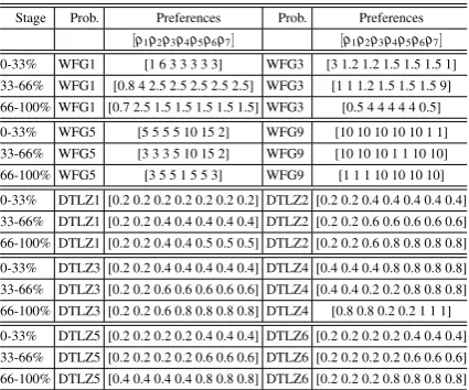
The preference vectors, for each benchmark prob-lem, are displayed in Table 1, wheremrefers to a spe-cific objective for the multi-objective problem.

Table 1. Preference Vectors throughout the optimisation process

Stage Prob. Preferences Prob. Preferences

[ρ1ρ2ρ3ρ4ρ5ρ6ρ7] [ρ1ρ2ρ3ρ4ρ5ρ6ρ7] 0-33% WFG1 [1 6 3 3 3 3 3] WFG3 [3 1.2 1.2 1.5 1.5 1.5 1]

33-66% WFG1 [0.8 4 2.5 2.5 2.5 2.5 2.5] WFG3 [1 1 1.2 1.5 1.5 1.5 9]

66-100% WFG1 [0.7 2.5 1.5 1.5 1.5 1.5 1.5] WFG3 [0.5 4 4 4 4 4 0.5]

0-33% WFG5 [5 5 5 5 10 15 2] WFG9 [10 10 10 10 10 1 1]

33-66% WFG5 [3 3 3 5 10 15 2] WFG9 [10 10 10 1 1 10 10]

66-100% WFG5 [3 5 5 1 5 5 3] WFG9 [1 1 1 10 10 10 10]

0-33% DTLZ1 [0.2 0.2 0.2 0.2 0.2 0.2 0.2] DTLZ2 [0.2 0.2 0.4 0.4 0.4 0.4 0.4]

33-66% DTLZ1 [0.2 0.2 0.4 0.4 0.4 0.4 0.4] DTLZ2 [0.2 0.2 0.6 0.6 0.6 0.6 0.6]

66-100% DTLZ1 [0.2 0.2 0.4 0.4 0.5 0.5 0.5] DTLZ2 [0.2 0.2 0.6 0.8 0.8 0.8 0.8]

0-33% DTLZ3 [0.2 0.2 0.4 0.4 0.4 0.4 0.4] DTLZ4 [0.4 0.4 0.4 0.8 0.8 0.8 0.8]

33-66% DTLZ3 [0.2 0.2 0.6 0.6 0.6 0.6 0.6] DTLZ4 [0.4 0.4 0.2 0.2 0.8 0.8 0.8]

66-100% DTLZ3 [0.2 0.2 0.6 0.8 0.8 0.8 0.8] DTLZ4 [0.8 0.8 0.2 0.2 1 1 1]

0-33% DTLZ5 [0.2 0.2 0.2 0.2 0.4 0.4 0.4] DTLZ6 [0.2 0.2 0.2 0.2 0.4 0.4 0.4]

33-66% DTLZ5 [0.2 0.2 0.2 0.2 0.6 0.6 0.6] DTLZ6 [0.2 0.2 0.2 0.2 0.6 0.6 0.6]

66-100% DTLZ5 [0.4 0.4 0.4 0.4 0.8 0.8 0.8] DTLZ6 [0.2 0.2 0.2 0.8 0.8 0.8 0.8]

At each stage of the optimisation, the preference vector P defined by the DM (each of them specified in Table 1) is the reference point for the hypervolume indicator.

3.2. Experimental Results

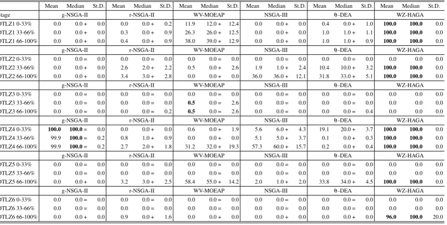
The numerical results for the ten seven-objective op-timisation test-cases have been listed in Table 1, these have been divided according to the two performance characteristics mentioned above.

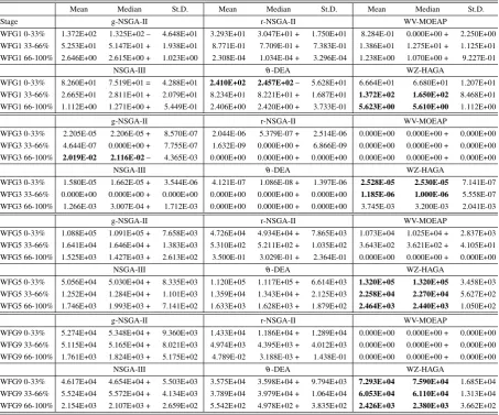
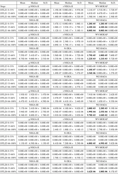
The performance of the algorithms in terms of the hypervolume indicator values is displayed in Tables 2 and 3, for WFG and DTLZ problems respectively, whilst the performance in terms of the number of so-lutions within the ROI is reported in Tables 4 and 5 re-spectively. In each table, mean (Mean), median (Me-dian) and standard deviation (St.D.) values are dis-played. The best results are emphasised in bold.

In order to verify the statistical significance of the results, the Wilcoxon signed-rank test [69] has been performed on the mean values where WZ-HAGA is taken as the reference. The statistical significance is indicated with a “+” when WZ-HAGA outperforms its competitor and with a “–” when WZ-HAGA is outperformed. A “=” indicates that there is no out-performance.

As shown in Table 2, the proposed WZ-HAGA achieves the best performance, regarding hypervolume values on WFG problems, this holds true in the ma-jority of the test-cases (it is outperformed only twice out of twelve times). In all the other test-cases the pro-posed WZ-HAGA significantly outperforms all of its competitors. Specifically,θ-DEA exhibits higher hy-pervolume performance in terms of mean and median values compared to WZ-HAGA in only the first stage of optimisation (0-33%) for the WFG1 test problem. A similar behavior can be observed for the g-NSGA-II in the last stage of evolution (66-100%) for the WFG3 test problem.

Table 2. WFG Test-case Hypervolume Results

Mean Median St.D. Mean Median St.D. Mean Median St.D.

Stage g-NSGA-II r-NSGA-II WV-MOEAP

WFG1 0-33% 1.372E+02 1.325E+02 – 4.648E+01 3.293E+01 3.047E+01 + 1.750E+01 8.284E-01 0.000E+00 + 2.250E+00 WFG1 33-66% 5.253E+01 5.147E+01 + 1.938E+01 8.771E-01 7.709E-01 + 7.383E-01 1.386E+01 1.275E+01 + 1.125E+01 WFG1 66-100% 2.646E+00 2.615E+00 + 1.023E+00 2.308E-04 1.034E-04 + 3.296E-04 1.238E+00 1.070E+00 + 9.227E-01

NSGA-III θ-DEA WZ-HAGA

WFG1 0-33% 8.260E+01 7.519E+01 = 4.288E+01 2.410E+02 2.457E+02– 5.628E+01 6.664E+01 6.680E+01 1.207E+01 WFG1 33-66% 2.665E+01 2.811E+01 + 2.079E+01 8.234E+01 8.221E+01 + 1.687E+01 1.372E+02 1.650E+02 8.468E+01 WFG1 66-100% 1.112E+00 1.271E+00 + 5.449E-01 2.406E+00 2.420E+00 + 3.733E-01 5.623E+00 5.610E+00 1.112E+00

g-NSGA-II r-NSGA-II WV-MOEAP

WFG3 0-33% 2.205E-05 2.206E-05 + 8.570E-07 2.044E-06 5.379E-07 + 2.514E-06 0.000E+00 0.000E+00 + 0.000E+00 WFG3 33-66% 4.644E-07 0.000E+00 + 7.755E-07 1.632E-09 0.000E+00 + 6.866E-09 0.000E+00 0.000E+00 + 0.000E+00 WFG3 66-100% 2.019E-02 2.116E-02– 4.365E-03 0.000E+00 0.000E+00 + 0.000E+00 0.000E+00 0.000E+00 + 0.000E+00

NSGA-III θ-DEA WZ-HAGA

WFG3 0-33% 1.580E-05 1.662E-05 + 3.544E-06 4.121E-07 1.086E-08 + 1.397E-06 2.528E-05 2.530E-05 7.141E-07 WFG3 33-66% 0.000E+00 0.000E+00 + 0.000E+00 0.000E+00 0.000E+00 + 0.000E+00 1.185E-06 1.000E-06 5.558E-07 WFG3 66-100% 1.266E-03 3.007E-04 + 1.712E-03 0.000E+00 0.000E+00 + 0.000E+00 3.745E-03 3.200E-03 2.041E-03

g-NSGA-II r-NSGA-II WV-MOEAP

WFG5 0-33% 1.088E+05 1.091E+05 + 7.658E+03 4.726E+04 4.934E+04 + 7.865E+03 1.073E+04 1.025E+04 + 2.837E+03

WFG5 33-66% 1.641E+04 1.646E+04 + 1.383E+03 5.310E+02 5.211E+02 + 1.035E+02 3.643E+02 3.621E+02 + 4.105E+01 WFG5 66-100% 1.525E+03 1.427E+03 + 2.613E+02 3.500E-01 3.029E-01 + 2.364E-01 0.000E+00 0.000E+00 + 0.000E+00

NSGA-III θ-DEA WZ-HAGA

WFG5 0-33% 5.056E+04 5.030E+04 + 8.335E+03 1.120E+05 1.117E+05 + 6.614E+03 1.320E+05 1.320E+05 3.458E+03 WFG5 33-66% 1.252E+04 1.284E+04 + 1.101E+03 1.359E+04 1.343E+04 + 2.125E+03 2.258E+04 2.270E+04 5.627E+02 WFG5 66-100% 1.746E+03 1.993E+03 + 7.141E+02 1.633E+03 1.628E+03 + 1.879E+02 2.464E+03 2.440E+03 1.050E+02

g-NSGA-II r-NSGA-II WV-MOEAP

WFG9 0-33% 5.274E+04 5.348E+04 + 9.360E+03 1.433E+04 1.186E+04 + 1.289E+04 0.000E+00 0.000E+00 + 0.000E+00 WFG9 33-66% 5.115E+04 5.165E+04 + 8.021E+03 4.974E+03 4.395E+03 + 4.012E+03 0.000E+00 0.000E+00 + 0.000E+00

WFG9 66-100% 1.761E+03 1.824E+03 + 5.175E+02 4.789E-02 3.188E-03 + 1.438E-01 0.000E+00 0.000E+00 + 0.000E+00

NSGA-III θ-DEA WZ-HAGA

WFG9 0-33% 4.617E+04 4.654E+04 + 5.503E+03 3.575E+04 3.598E+04 + 9.794E+03 7.293E+04 7.590E+04 1.685E+04 WFG9 33-66% 5.524E+04 5.572E+04 + 4.134E+03 3.789E+04 3.979E+04 + 1.064E+04 6.053E+04 6.110E+04 1.313E+04 WFG9 66-100% 2.154E+03 2.107E+03 + 2.659E+02 5.542E+02 4.978E+02 + 3.835E+02 2.426E+03 2.380E+03 3.662E+02

The numerical results listed in Table 4, in terms of the number of solutions within the ROI, show that WZ-HAGA outperforms all its competitors in the ma-jority of the WFG problems considered. In the major-ity of the cases, WZ-HAGA is able to maintain its pop-ulation within the ROI. The proposed WZ-HAGA is outperformed only by g-NSGA-II for the WFG1 prob-lem (first two stages: 0-33%, and 33-66%). The results in listed Table 5 show that WZ-HAGA is never outper-formed on the DTLZ problems.

Fig. 3 and 4 show two examples of the trend of average (over the 30 runs) hypervolume indicator val-ues and numbers of solutions within the ROI, during the optimisation process. Fig. 3 shows the evolution

for WFG9, while Fig. 4 shows the performance pa-rameters for DTLZ4. In each figure, the upper three subplots show the hypervolume variation in the three stages of the optimisation, while the lower three sub-plots show the variation of the number of solutions falling within the ROI.

Table 3. DTLZ Test-case Hypervolume Results

Mean Median St.D. Mean Median St.D. Mean Median St.D.

Stage g-NSGA-II r-NSGA-II WV-MOEAP

DTLZ1 0-33% 0.00E+00 0.00E+00 + 0.00E+00 1.19E-08 0.00E+00 + 5.97E-08 3.21E-07 4.51E-08 + 3.72E-07 DTLZ1 33-66% 0.00E+00 0.00E+00 + 0.00E+00 6.93E-06 0.00E+00 + 2.18E-05 6.81E-05 6.67E-05 + 1.61E-05 DTLZ1 66-100% 0.00E+00 0.00E+00 + 0.00E+00 1.48E-05 0.00E+00 + 4.32E-05 1.58E-04 1.46E-04 + 2.30E-05

NSGA-III θ-DEA WZ-HAGA

DTLZ1 0-33% 0.00E+00 0.00E+00 + 0.00E+00 3.47E-12 0.00E+00 + 1.08E-11 1.28E-05 1.28E-05 0.00E+00 DTLZ1 33-66% 0.00E+00 0.00E+00 + 0.00E+00 1.08E-13 3.93E-19 + 2.79E-13 4.10E-04 4.10E-04 0.00E+00 DTLZ1 66-100% 0.00E+00 0.00E+00 + 0.00E+00 1.12E-11 3.34E-17 + 5.18E-11 8.00E-04 8.00E-04 0.00E+00

g-NSGA-II r-NSGA-II WV-MOEAP

DTLZ2 0-33% 0.00E+00 0.00E+00 = 0.00E+00 0.00E+00 0.00E+00 = 0.00E+00 0.00E+00 0.00E+00 = 0.00E+00 DTLZ2 33-66% 0.00E+00 0.00E+00 + 0.00E+00 1.16E-10 2.38E-11 + 1.97E-10 8.63E-08 0.00E+00 + 4.32E-07 DTLZ2 66-100% 0.00E+00 0.00E+00 + 0.00E+00 4.89E-14 5.79E-15 + 8.94E-14 0.00E+00 0.00E+00 + 0.00E+00

NSGA-III θ-DEA WZ-HAGA

DTLZ2 0-33% 0.00E+00 0.00E+00 = 0.00E+00 0.00E+00 0.00E+00 = 0.00E+00 0.00E+00 0.00E+00 0.00E+00 DTLZ2 33-66% 7.55E-07 5.41E-07 + 1.01E-06 3.56E-08 2.53E-08 + 3.72E-08 1.79E-05 1.80E-05 7.60E-07 DTLZ2 66-100% 8.75E-04 9.00E-04 + 2.51E-04 3.23E-06 2.29E-06 + 2.53E-06 1.22E-03 1.21E-03 5.72E-05

g-NSGA-II r-NSGA-II WV-MOEAP

DTLZ3 0-33% 0.00E+00 0.00E+00 = 0.00E+00 0.00E+00 0.00E+00 = 0.00E+00 0.00E+00 0.00E+00 = 0.00E+00 DTLZ3 33-66% 0.00E+00 0.00E+00 = 0.00E+00 0.00E+00 0.00E+00 = 0.00E+00 1.10E-07 0.00E+00 = 5.51E-07 DTLZ3 66-100% 0.00E+00 0.00E+00 = 0.00E+00 1.49E-07 0.00E+00 = 7.47E-07 2.54E-06 0.00E+00 = 1.27E-05

NSGA-III θ-DEA WZ-HAGA

DTLZ3 0-33% 0.00E+00 0.00E+00 = 0.00E+00 0.00E+00 0.00E+00 = 0.00E+00 0.00E+00 0.00E+00 0.00E+00 DTLZ3 33-66% 0.00E+00 0.00E+00 = 0.00E+00 0.00E+00 0.00E+00 = 0.00E+00 0.00E+00 0.00E+00 0.00E+00 DTLZ3 66-100% 0.00E+00 0.00E+00 = 0.00E+00 9.15E-12 0.00E+00 = 4.57E-11 0.00E+00 0.00E+00 0.00E+00

g-NSGA-II r-NSGA-II WV-MOEAP

DTLZ4 0-33% 1.93E-03 1.92E-03 = 1.47E-04 0.00E+00 0.00E+00 + 0.00E+00 7.91E-06 0.00E+00 + 2.62E-05 DTLZ4 33-66% 1.49E-04 1.45E-04 = 1.82E-05 2.47E-07 7.82E-09 + 5.50E-07 0.00E+00 0.00E+00 + 0.00E+00 DTLZ4 66-100% 6.47E-03 6.41E-03 + 4.59E-04 1.35E-09 4.41E-10 + 2.44E-09 1.76E-03 1.65E-03 + 9.35E-04

NSGA-III θ-DEA WZ-HAGA

DTLZ4 0-33% 3.17E-04 2.41E-04 + 2.90E-04 4.05E-04 4.18E-04 + 9.82E-05 2.08E-03 2.20E-03 9.19E-04 DTLZ4 33-66% 3.94E-05 3.69E-05 + 2.75E-05 4.54E-07 0.00E+00 + 1.61E-06 1.99E-04 2.55E-04 8.70E-05 DTLZ4 66-100% 8.34E-03 8.60E-03 + 1.78E-03 1.01E-04 0.00E+00 + 2.82E-04 9.78E-03 1.04E-02 1.68E-03

g-NSGA-II r-NSGA-II WV-MOEAP

DTLZ5 0-33% 0.00E+00 0.00E+00 = 0.00E+00 0.00E+00 0.00E+00 = 0.00E+00 0.00E+00 0.00E+00 = 0.00E+00 DTLZ5 33-66% 0.00E+00 0.00E+00 = 0.00E+00 0.00E+00 0.00E+00 = 0.00E+00 0.00E+00 0.00E+00 = 0.00E+00 DTLZ5 66-100% 0.00E+00 0.00E+00 + 0.00E+00 2.44E-15 1.00E-15 + 4.14E-15 2.79E-05 2.79E-05 + 5.95E-09

NSGA-III θ-DEA WZ-HAGA

DTLZ5 0-33% 0.00E+00 0.00E+00 = 0.00E+00 0.00E+00 0.00E+00 = 0.00E+00 0.00E+00 0.00E+00 0.00E+00 DTLZ5 33-66% 0.00E+00 0.00E+00 = 0.00E+00 0.00E+00 0.00E+00 = 0.00E+00 0.00E+00 0.00E+00 0.00E+00 DTLZ5 66-100% 1.13E-05 6.59E-06 + 1.15E-05 8.41E-06 7.20E-06 + 5.29E-06 6.88E-05 6.99E-05 5.82E-06

g-NSGA-II r-NSGA-II WV-MOEAP

DTLZ6 0-33% 0.00E+00 0.00E+00 = 0.00E+00 0.00E+00 0.00E+00 = 0.00E+00 0.00E+00 0.00E+00 = 0.00E+00 DTLZ6 33-66% 0.00E+00 0.00E+00 = 0.00E+00 0.00E+00 0.00E+00 = 0.00E+00 0.00E+00 0.00E+00 = 0.00E+00 DTLZ6 66-100% 0.00E+00 0.00E+00 + 0.00E+00 2.70E-12 0.00E+00 + 6.53E-12 0.00E+00 0.00E+00 + 0.00E+00

NSGA-III θ-DEA WZ-HAGA

Table 4. WFG Test-case ROI Results

Mean Median St.D. Mean Median St.D. Mean Median St.D. Mean Median St.D. Mean Median St.D. Mean Median St.D.

Stage g-NSGA-II r-NSGA-II WV-MOEAP NSGA-III θ-DEA WZ-HAGA

WFG1 0-33% 100.0 100.0– 0.0 31.2 29.0 + 6.5 2.0 0.0 + 4.4 14.8 15.0 + 9.1 95.8 98.0 = 7.1 94.0 96.0 5.6 WFG1 33-66% 100.0 100.0– 0.0 5.6 6.0 + 3.5 10.2 13.0 + 5.1 7.6 5.0 + 8.0 82.6 85.0 + 10.0 91.9 100.0 11.3 WFG1 66-100% 100.0 100.0= 0.0 6.3 4.0 + 6.4 13.0 13.0 + 0.0 11.0 12.0 + 8.8 47.3 47.0 + 6.1 100.0 100.0 0.0

g-NSGA-II r-NSGA-II WV-MOEAP NSGA-III θ-DEA WZ-HAGA

WFG3 0-33% 100.0 100.0= 0.0 2.0 2.0 + 1.041 0.0 0.0 + 0.0 46.2 49.0 + 13.8 1.9 2.0 + 1.4 100.0 100.0 0.0 WFG3 33-66% 28.0 0.0 + 45.8 0.4 0.0 + 0.645 0.0 0.0 + 0.0 0.0 0.0 + 0.0 0.0 0.0 + 0.0 100.0 100.0 0.0 WFG3 66-100% 96.0 100.0= 20.0 0.0 0.0 + 0.000 0.0 0.0 + 0.0 0.8 1.0 + 1.1 0.0 0.0 + 0.0 100.0 100.0 0.0

g-NSGA-II r-NSGA-II WV-MOEAP NSGA-III θ-DEA WZ-HAGA

WFG5 0-33% 100.0 100.0= 0.0 39.4 40.0 + 6.0 89.4 91.0 + 4.3 57.4 55.0 + 14.1 58.1 59.0 + 8.8 100.0 100.0 0.0 WFG5 33-66% 100.0 100.0= 0.0 41.1 42.0 + 11.5 90.5 91.0 + 2.6 66.0 69.0 + 13.6 36.6 37.0 + 8.5 100.0 100.0 0.0 WFG5 66-100% 99.9 100.0= 0.2 16.1 15.0 + 10.1 0.0 0.0 + 0.0 16.2 16.0 + 8.2 28.8 28.0 + 7.4 100.0 100.0 0.0

g-NSGA-II r-NSGA-II WV-MOEAP NSGA-III θ-DEA WZ-HAGA

WFG9 0-33% 100.0 100.0= 0.0 3.7 3.0 + 2.2 0.0 0.0 + 0.0 46.7 47.0 + 9.8 14.2 14.0 + 5.5 100.0 100.0 0.0 WFG9 33-66% 100.0 100.0= 0.0 4.6 4.0 + 2.8 0.0 0.0 + 0.0 53.4 53.0 + 6.4 17.2 17.0 + 5.5 100.0 100.0 0.0 WFG9 66-100% 100.0 100.0= 0.0 2.0 1.0 + 2.5 0.0 0.0 + 0.0 57.4 58.0 + 5.4 6.7 6.0 + 4.2 100.0 100.0 0.0

Table 5. DTLZ Test-case ROI Results

Mean Median St.D. Mean Median St.D. Mean Median St.D. Mean Median St.D. Mean Median St.D. Mean Median St.D.

Stage g-NSGA-II r-NSGA-II WV-MOEAP NSGA-III θ-DEA WZ-HAGA

DTLZ1 0-33% 0.0 0.0 + 0.0 0.0 0.0 + 0.2 11.9 12.0 + 12.4 0.0 0.0 + 0.0 0.4 0.0 + 1.0 100.0 100.0 0.0 DTLZ1 33-66% 0.0 0.0 + 0.0 0.3 0.0 + 0.9 26.3 26.0 + 12.5 0.0 0.0 + 0.0 1.0 1.0 + 1.1 100.0 100.0 0.0 DTLZ1 66-100% 0.0 0.0 + 0.0 0.4 0.0 + 0.9 38.0 39.0 + 12.9 0.0 0.0 + 0.0 1.0 1.0 + 0.9 100.0 100.0 0.0

g-NSGA-II r-NSGA-II WV-MOEAP NSGA-III θ-DEA WZ-HAGA

DTLZ2 0-33% 0.0 0.0 = 0.0 0.0 0.0 = 0.0 0.0 0.0 = 0.0 0.0 0.0 = 0.0 0.0 0.0 = 0.0 0.0 0.0 0.0 DTLZ2 33-66% 0.0 0.0 + 0.0 2.6 2.0 + 2.2 0.5 0.0 + 2.6 1.9 1.0 + 2.4 10.4 10.0 + 3.2 100.0 100.0 0.0 DTLZ2 66-100% 0.0 0.0 + 0.0 3.4 3.0 + 2.8 0.0 0.0 + 0.0 36.0 36.0 + 12.1 31.8 33.0 + 5.1 100.0 100.0 0.0

g-NSGA-II r-NSGA-II WV-MOEAP NSGA-III θ-DEA WZ-HAGA

DTLZ3 0-33% 0.0 0.0 = 0.0 0.0 0.0 = 0.0 0.0 0.0 = 0.0 0.0 0.0 = 0.0 0.0 0.0 = 0.0 0.0 0.0 0.0 DTLZ3 33-66% 0.0 0.0 = 0.0 0.0 0.0 = 0.0 0.5 0.0 = 2.6 0.0 0.0 = 0.0 0.0 0.0 = 0.0 0.0 0.0 0.0 DTLZ3 66-100% 0.0 0.0 = 0.0 0.0 0.0 = 0.2 0.5 0.0 = 2.6 0.0 0.0 = 0.0 0.0 0.0 = 0.4 0.0 0.0 0.0

g-NSGA-II r-NSGA-II WV-MOEAP NSGA-III θ-DEA WZ-HAGA

DTLZ4 0-33% 100.0 100.0= 0.0 0.0 0.0 + 0.0 0.6 0.0 + 1.9 5.6 6.0 + 4.3 19.1 20.0 + 3.7 100.0 100.0 0.0 DTLZ4 33-66% 99.9 100.0= 0.2 0.8 1.0 + 0.9 0.0 0.0 + 0.0 5.1 5.0 + 3.7 0.1 0.0 + 0.3 100.0 100.0 0.0 DTLZ4 66-100% 99.9 100.0= 0.2 2.7 2.0 + 1.8 31.2 32.0 + 19.3 57.3 60.0 + 15.7 0.2 0.0 + 0.4 100.0 100.0 0.0

g-NSGA-II r-NSGA-II WV-MOEAP NSGA-III θ-DEA WZ-HAGA

DTLZ5 0-33% 0.0 0.0 = 0.0 0.0 0.0 = 0.0 0.0 0.0 = 0.0 0.0 0.0 = 0.0 0.0 0.0 = 0.0 0.0 0.0 0.0 DTLZ5 33-66% 0.0 0.0 = 0.0 0.0 0.0 = 0.0 0.0 0.0 = 0.0 0.0 0.0 = 0.0 0.0 0.0 = 0.0 0.0 0.0 0.0 DTLZ5 66-100% 0.0 0.0 + 0.0 3.2 3.0 + 2.5 58.4 55.0 + 14.2 2.0 1.0 + 2.0 33.8 34.0 + 4.5 100.0 100.0 0.0

g-NSGA-II r-NSGA-II WV-MOEAP NSGA-III θ-DEA WZ-HAGA

DTLZ6 0-33% 0.0 0.0 = 0.0 0.0 0.0 = 0.0 0.0 0.0 = 0.0 0.0 0.0 = 0.0 0.0 0.0 = 0.0 0.0 0.0 0.0 DTLZ6 33-66% 0.0 0.0 = 0.0 0.0 0.0 = 0.0 0.0 0.0 = 0.0 0.0 0.0 = 0.0 0.0 0.0 = 0.0 0.0 0.0 0.0 DTLZ6 66-100% 0.0 0.0 + 0.0 0.9 0.0 + 1.6 0.0 0.0 + 0.0 0.0 0.0 + 0.0 0.0 0.0 + 0.0 96.0 100.0 20.0

from this drop and achieves higher values, thus dis-playing resilient and robust behaviour. Some other al-gorithms, such as WV-MOEAP, appear to be unable to recover from the change in the preference vector af-ter some initial improvements in the hypervolume val-ues. NSGA-III and g-NSGA-II also display resilient behaviour, although they are outperformed by WZ-HAGA in this regard.

The results in terms of solutions in the ROI show that WZ-HAGA and g-NSGA-II display a similar per-formance. For the specific problem, both these

algo-rithms rapidly produce a population entirely within the ROI within the first 50 generations. This is because they both explicitly employ information regarding the preference vector within their search. The NSGA-III algorithm also displays good performance. According to our interpretations, this fact is due to the NSGA-III logic that encodes some DM information through its reference vector, and then makes an implicit use of it during the search.

Figure 3. (a-c) Mean hypervolume quality of the considered algorithms at each generation of the test-cases: WFG9 (0–33%), WFG9 (33–66%), and WFG9 (66–100%); (d-f) Mean number of solutions within the ROI for each of the considered algorithms at each generation of the test-cases WFG9 (00–33%), WFG9 (33–66%), and WFG9 (66–100%).

0

100

200

300

Generations

0

1

2

Hypervolume

1e 3 (a) Mean Hypervolume

g-NSGA-II r-NSGA-II WV-MOEA-P NSGA-III Θ-DEA WZ-HAGA

0

100

200

300

Generations

0

50

100

No. Solutions in ROI

(d) Mean ROI Solutions

400

500

600

Generations

0.0

0.5

1.0

1.5

1e 4 (b) Mean Hypervolume

400

500

600

Generations

0

50

100

(e) Mean ROI Solutions

700

800

900

Generations

0.0

0.5

1e 2 (c) Mean Hypervolume

700

800

900

1000

Generations

0

50

100

(f) Mean ROI Solutions

Figure 4. (a-c) Mean hypervolume quality of the considered algorithms at each generation of the test-cases: DTLZ4 (0–33%), DTLZ4 (33–66%), and DTLZ4 (66–100%); (d-f) Mean number of solutions within the ROI for each of the considered algorithms at each generation of the test-cases DTLZ4 (0–33%), DTLZ4 (33–66%), and DTLZ4 (66–100%).

the early generations (0-33%). It can be observed that g-NSGA-II is faster than WZ-HAGA in reaching a high hypervolume indicator value and at getting the

Pitch Axis

Yaw Axis

Roll Axis + Pitch

+ Roll

+ Yaw Centre of Gravity

Figure 5.The three main axes of an Aircraft body.

clearly visible for the hypervolume results. While g-NSGA-II drops in hypervolume performance and does not appear to recover, WZ-HAGA quickly reaches higher hypervolume values.

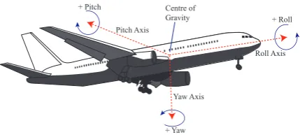
3.3. Preference Articulation in the Design of a Fighter Vehicle Control System

In order to demonstrate the practical usability of the proposed WZ-HAGA, it has been applied to the de-sign of the flying control system of a fighter vehicle (aircraft). Fig. 5 presents an illustration of an aircraft with the three main axes of motion labelled: the Roll (longitudinal) axisr, the Pitch (lateral) axisp, and the Yaw (vertical) axisy. Three angles (rate) can be asso-ciated to the position of the aircraft to characterise it. Furthermore, two more important parameters describe the behavior of an airplane in flying conditions. The first is the sideslip angleβ that is the rotation angle of the nose of the airplane due to the relative wind, see [63]. The second one is the bank angleφ, that is a met-ric related to the speed (and performance) of the air-plane and is measured in (aperiodic) degrees, see [21] for details.

From the perspective of this work, an aircraft is characterised by the following (time-dependent) state vectorxand controller vectoru:

x= 

  

β

y r

φ



  

,u=

δα

δr

,

whereyandrare the yaw and roll rates, respectively,

δα is the aileron control motions andδr is the rudder control motions.

The control vector is also expressed as:u=Cup+ Kx, whereup is the pilot’s control input vector here

set as[12,0],CandKare the gain matrices:

C=

1 0 k51

,K=

k6k1k20 k7k3k40

.

The control problem under study consists of find-ing those gain coefficientsκ= [k1,k2,k3,k4,k5,k6,k7] that simultaneously minimise the following seven ob-jectives (in their qualitative definition):

f1(κ): The spiral root

f2(κ): The damping in roll root

f3(κ): The dutch-roll damping ratio

f4(κ): The dutch-roll frequency

f5(κ): The bank angle at 1 seconds

f6(κ): The bank angle at 2.8 seconds

f7(κ): The control effort

The first four objectives in the list refer to unde-sired oscillations of the airplane, the fifth and and sixth objectives refer to the position of the airplane in cru-cial moments of the flight according to Military Spec-ification [5,20], the last objective refers to the fact that small gains in absolute values are preferred to guar-antee the stability of the controller. Details about the controller can be found in [63].

In order to give a mathematically rigorous de-scription of the multi-objective optimisation problem, let us consider the kinetic energy matrix A and the Coriolis matrix B. In the problem under investiga-tion, these two matrices are composed of constant el-ements (describing the mechanics of the airplane in [63]) given by:

A= 

  

−0.2842−0.9879 0.1547 0.0204 10.8574−0.5504−0.2896 0.0000

−199.8942−0.4840−1.6025 0.0000 0.0000 0.1566 1.0000 0.0000



  

,

B= 

  

0.0000 0.0524 0.4198−12.7393 50.5756 21.6753 0.0000 0.0000



  

.

f2(κ), f3(κ), and f4(κ)and the eigenvalues of the

4×4 matrixD. It can be observed that the eigenvalue expressions depend on the gain coefficients in the ma-trixKwhile all the other parameters are constant.

The objective functions f5(κ)and f6(κ)are the bank angles taken at two specific times, 1 and 2.8 sec-onds. Since the bankφis time-variant, it can be seen as a function of timeφ(t). Thanks to the linearisation de-scribed in [42], the bank at a specified moment (1 and 2.8 seconds) can be expressed as function of the gain coefficients. These functions of the linearised model are the objective functions f5(κ)and f6(κ)we used

in this study. For further details see [63].

The objective functions f7(κ) is the sum of

squares of the gain coefficients:

f7(κ) =

7

∑

k2_i.

Further details regarding the aircraft dynamic model and the problem variables are available in [20]. This optimisation problem will be referred to as Lat-eral Controller Synthesis (LATCON) herein.

By using the same notation above, the preferences of the LATCON problem are displayed in Table 6.

Table 6. LATCON preference vectors

Preferences

Stage [ρ1ρ2ρ3ρ4ρ5ρ6ρ7]

00–33% [-0.01 -3.75 -0.45 -1 -90 -360 0.75]

33–66% [-0.01 -3.75 -0.45 -1 -90 -500 0.25] 66–100% [-0.01 -3.75 -0.45 -1-200 -1500 0.25]

Although a detailed explanation of the physical problem does not fall within the scopes of this arti-cle, what follows is a brief explanation of the prefer-ence vectors in Table 6. Mathematically, the meaning of the preference vector is that each objective function fimust be below the corresponding valueρi, fori= 1,2, . . . ,7. The first four values of P, i.e.ρ1,ρ2,ρ3,ρ4 are all negative numbers which are not changed during the optimisation.

From an engineering perspective, negative eigen-values (in their real part) lead to a stable control system but a higher performance is generally obtained when the eigenvalues are close to the imaginary axis. We are fixing a range that guarantees stability and a

min-imal performance of the control system (given by the

ρ1,ρ2,ρ3,ρ4 values). Since moving these values dur-ing the optimisation could likely lead to movdur-ing the search toward the instability region, these values are kept constant. However, a dynamic increasing perfor-mance requirement is performed by the preference ar-ticulation on f7. Since the function is positive definite,

ρ7is a positive number. While initially solutions with poorer performance are taken into account, after 33% of the optimisation budget, the search becomes bi-ased towards more restrictive DM requirements. This choice has been made to ensure that, at first, the algo-rithm produces stable solutions and then refines them within the stability region. The parametersρ5andρ6 represent the bank angles in degrees in two specific moments. The negative sign is conventional (the abso-lute value is relevant and the sign is used in the min-imisation). Here, we are simulating a scenario where the DM initially attempts to impose more restrictive requirements by the reducing the rotation range at 6 seconds after 33% of the budget and then, due to other external considerations, decides to radically modify their requirements after 66% of the budget, e.g. due to the change in the control strategy. With the last varia-tion we are interested in checking how the algorithms can react to abrupt changes of the ROI.

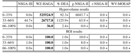
The same algorithms presented above with the same parameter setting above have been applied. The numerical results in terms of the hypervolume and so-lutions belonging within the ROI (mean values and Wilcoxon signed-rank test [69]) are displayed in Table 7. A graphical representation of the LATCON results is displayed in Fig. 6.

Table 7. LATCON Hypervolume and ROI Results

NSGA-III WZ-HAGA θ-DEA g-NSGA-II r-NSGA-II WV-MOEAP Hypervolume results

0–33% 0.0+ 525524.9 92.3+ 6043.7 + 0.0 + 0.0 + 33–66% 44.7+ 26717.8 1125.9+ 63.9 + 0.0 + 0.0 + 66–100% 0.0+ 36.0 2.4+ 0.0 + 0.0 + 0.0 +

ROI results

0–33% 0.0+ 100.0 1.0+ 10.0 + 0.0 + 0.0 + 33–66% 1.0+ 100.0 1.0+ 8.0 + 0.0 + 0.0 + 66–100% 0.0+ 100.0 1.0+ 0.0 + 0.0 + 0.0 +

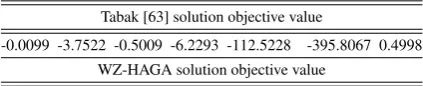
been then compared against those obtained by one of the four solutions detected by the method originally proposed in [63]. These results are displayed in Ta-ble 8. It can be observed that the WZ-HAGA solution dominates the solution found in [63].

Table 8. Comparison with results from the original article

Tabak [63] solution objective value

-0.0099 -3.7522 -0.5009 -6.2293 -112.5228 -395.8067 0.4998 WZ-HAGA solution objective value

-0.1027 -5.0808 -0.7152 -7.1043 -202.1296 -1523.4950 0.2244

The results suggest that WZ-HAGA is able to quickly (within a few generations) find solutions within the ROI and continue to converge towards an approximation set which dominates more of the ob-jective space. Following the beginning of each change in DM preferences, it can be observed that the entire population has converged to being within the ROI af-ter at most ten subsequent generations. The reaction of the hypervolume indicator is slower but steadily grows within each stage and reaches the highest value, see Fig. 6.

The competitor algorithms, on this problem, dis-play a significantly poorer performance than the pro-posed WZ-HAGA. The main limitation of these algo-rithms, including those that make use of progressive preference articulation, is that they appear to be unable to find enough solutions within the ROI.

4. Conclusion

This paper introduces a method for progressive pref-erence articulation based on statistical theory used in a priori preference articulation, and integrates it within a previously proposed algorithmic framework for multi-objective optimisation. The proposed algo-rithmic component checks the number of solutions within the ROI indicated by the DM, and biases the search towards the ROI when not enough solutions are pertinent. An adaptive mechanism modifies the bias on the basis of the number of solutions within the region of interest, thus reacting every time the decision mak-ing circumstances change. A novel implementation of a complete algorithm for interactive multi-objective optimisation (WZ-HAGA) is then proposed.

The proposed WZ-HAGA has been thoroughly tested against five modern algorithms on a number of test problems and a real-world test-case. The nu-merical results show that the proposed method signif-icantly outperforms its competitors in eight problems out of the ten considered. In these eight test-cases WZ-HAGA outperforms its competitors in terms of both the hypervolume indicator and the number of detected solutions within the ROI. The proposed WZ-HAGA also outperforms the other algorithms when compared within the real-world control engineering application.

It was found that WZ-HAGA, which uses an ag-gressive and targeted approach to selection pressure, is better suited to finding a ROI which has been defined by the DM’s preferences. In the presence of chang-ing preferences throughout the optimisation process, i.e. progressive preference articulation, WZ-HAGA quickly finds the new preferred solutions and outper-forms the considered algorithms in both the hypervol-ume indicator quality of the approximation set and the number of solutions found within the ROI.

References

[1] H. Adeli and K. C. Sarma,Cost Optimization of Structures: Fuzzy Logic, Genetic Algorithms, and Parallel Computing. New York, NY, USA: John Wiley & Sons, Inc., 2006. [2] S. F. Adra, I. Griffin, and P. J. Fleming, “A comparative study

of progressive preference articulation techniques for multiob-jective optimisation,” inEvolutionary Multi-Criterion Opti-mization, ser. Lecture Notes in Computer Science. Springer, 2007, vol. 4403, pp. 908–921.

[3] A. Auger, J. Bader, D. Brockhoff, and E. Zitzler, “Articulating user preferences in many-objective problems by sampling the weighted hypervolume,” inProceedings of the 11th Annual Conference on Genetic and Evolutionary Computation, ser. GECCO ’09. NY, USA: ACM, 2009, pp. 555–562. [4] K. Bhattacharjee, H. Singh, M. Ryan, and T. Ray, “Bridging

the gap: Many-objective optimization and informed decision-making,”IEEE Transactions on Evolutionary Computation, 2017, to appear.

[5] J. H. Blakelock,Automatic Control of Aircraft and Missiles. Wiley, 1965.

[6] A. Bolourchi, S. F. Masri, and O. J. Aldraihem, “Studies into Computational Intelligence and Evolutionary Approaches for Model-Free Identification of Hysteretic Systems,” Computer-Aided Civil & Infrastructure Engineering, vol. 30, no. 5, pp. 330–346, May 2015.

0

100

200

300

Generations

0

2

4

Hypervolume

1e5 (a) Mean Hypervolume

g-NSGA-II r-NSGA-II WV-MOEA-P NSGA-III Θ-DEA WZ-HAGA

0

100

200

300

Generations

0

50

100

No. Solutions in ROI

(d) Mean ROI Solutions

400

500

600

Generations

0

1

2

1e4 (b) Mean Hypervolume

400

500

600

Generations

0

50

100

(e) Mean ROI Solutions

700

800

900

1000

Generations

0

1

2

3

1e1 (c) Mean Hypervolume

700

800

900

1000

Generations

0

50

100

(f) Mean ROI Solutions

Figure 6. (a-c) Hypervolume quality of the considered algorithms at each generation of the different stages: 0–33%, 33–66%, and 66–100%; (d-f) Number of solutions within the ROI for each of the considered algorithms at each generation of the different stages 0–33%, 33–66%, and 66–100%.

[8] J. Branke and K. Deb, “Integrating user preferences into evo-lutionary multi-objective optimization,” inKnowledge Incor-poration in Evolutionary Computation, ser. Studies in Fuzzi-ness and Soft Computing, 2005, vol. 167, pp. 461–477. [9] M. A. Braun, P. K. Shukla, and H. Schmeck, “Preference

ranking schemes in multi-objective evolutionary algorithms,” inEvolutionary Multi-Criterion Optimization, ser. Lecture Notes in Computer Science. Springer, 2011, vol. 6576, pp. 226–240.

[10] A. Caponio and F. Neri, “Integrating cross-dominance adap-tation in multi-objective memetic algorithms,” in Multi-Objective Memetic Algorithms, ser. Studies in Computational Intelligence, Y.-S. Ong, K. C. Tan, and C.-K. Goh, Eds. Springer, 2009, vol. 171, pp. 325–351.

[11] A. Cerveira, J. Baptista, and E. J. S. Pires, “Wind farm dis-tribution network optimization,”Integrated Computer-Aided Engineering, vol. 23, no. 1, pp. 69–79, 2015.

[12] Y.-J. Cha and O. Buyukozturk, “Structural Damage Detection Using Modal Strain Energy and Hybrid Multiobjective Opti-mization,”Computer-Aided Civil & Infrastructure Engineer-ing, vol. 30, no. 5, pp. 347–358, May 2015.

[13] R. Cheng, M. Olhofer, and Y. Jin, “Reference vector based a posteriori preference articulation for evolutionary multiob-jective optimization,” inEvolutionary Computation (CEC), 2015 IEEE Congress on, May 2015, pp. 939–946.

[14] C. A. Coello Coello, “Handling preferences in evolution-ary multiobjective optimization: A survey,” inEvolutionary Computation, 2000. Proceedings of the 2000 Congress on, vol. 1. IEEE, 2000, pp. 30–37.

[15] K. Deb and H. Jain, “An evolutionary many-objective op-timization algorithm using reference-point-based nondomi-nated sorting approach, part i: Solving problems with box constraints,”Evolutionary Computation, IEEE Transactions on, vol. 18, no. 4, pp. 577–601, Aug 2014.

[16] K. Deb, “Multi-objective optimization,”Multi-objective opti-mization using evolutionary algorithms, pp. 13–46, 2001. [17] K. Deb, M. Mohan, and S. Mishra, “Evaluating the

-domination based multi-objective evolutionary algorithm for a quick computation of pareto-optimal solutions,” Evolution-ary Computation, vol. 13, no. 4, pp. 501–525, 2005. [18] K. Deb, J. Sundar, N. Udaya Bhaskara Rao, and S.

Chaud-huri, “Reference point based multi-objective optimization us-ing evolutionary algorithms,”International Journal of Com-putational Intelligence Research, vol. 2, no. 3, pp. 273–286, 2006.

[19] K. Deb, L. Thiele, M. Laumanns, and E. Zitzler, “Scal-able Test Problems for Evolutionary Multiobjective Opti-mization,” inEvolutionary Multiobjective Optimization, ser. Advanced Information and Knowledge Processing, A. Abra-ham, L. Jain, and R. Goldberg, Eds. Springer London, 2005, pp. 105–145, dOI: 10.1007/1-84628-137-7 6.

[20] B. Etkin,Dynamics of Atmospheric Flight. Wiley, 1972. [21] Federal Aviation Administration, “Faa: Air traffic plans and

publications,” 2017, archived: Change 3 April 27, 2017. [22] E. Filatovas, O. Kurasova, and K. Sindhya, “Synchronous

[23] E. Filatovas, A. Lanˇcinskas, O. Kurasova, and J. ˇZilinskas, “A preference-based multi-objective evolutionary algorithm r-nsga-ii with stochastic local search,”Central European Jour-nal of Operations Research, pp. 1–20, 2016.

[24] P. J. Fleming, R. C. Purshouse, and R. J. Lygoe, “Many objec-tive optimization: An engineering perspecobjec-tive,” in Proceed-ings of the International Conference on Evolutionary Multi-Objective Optimization (EMO2005), ser. Lecture Notes in Computer Science, C. A. Coello Coello, A. H. Aguirre, and E. Zitzler, Eds., vol. 3470. Springer, 2005, pp. 14 – 32. [25] C. M. Fonseca, “Preference articulation in evolutionary

mul-tiobjective optimisation,” in7th International Conference on Hybrid Intelligent Systems (HIS 2007), Sept 2007, pp. 4–4. [26] C. M. Fonseca and P. J. Fleming, “Genetic algorithms for

multi-objective optimization: Formulation, discussion and generalization,” in Proceedings of the Fifth International Conference on Genetic Algorithms, S. Forrest, Ed. Morgan Kaufmann, 1993, pp. 416–423.

[27] C. M. Fonseca and P. J. Fleming, “Multiobjective optimiza-tion and multiple constraint handling with evoluoptimiza-tionary algo-rithms - Part I: A unified formulation,”IEEE Transactions on Systems, Man, and Cybernetics - Part A: Systems and Hu-mans, vol. 28, no. 1, pp. 26 – 37, 1998.

[28] N. Hansen and A. Ostermeier, “Adapting arbitrary normal mutation distributions in evolution strategies: The covariance matrix adaptation,” inProceedings of IEEE International Conference on Evolutionary Computation, 1996. IEEE, 1996, pp. 312–317.

[29] H.-Z. Huang, Y.-K. Gu, and X. Du, “An interactive fuzzy multi-objective optimization method for engineering design,” Engineering Applications of Artificial Intelligence, vol. 19, no. 5, pp. 451 – 460, 2006.

[30] S. Huband, P. Hingston, L. Barone, and L. While, “A review of multiobjective test problems and a scalable test problem toolkit,”IEEE Transactions on Evolutionary Computation, vol. 10, no. 5, pp. 477–506, Oct. 2006.

[31] S. Huband, P. Hingston, L. Barone, and L. While, “A review of multiobjective test problems and a scalable test problem toolkit,”Evolutionary Computation, IEEE Transactions on, vol. 10, no. 5, pp. 477–506, 2006.

[32] G. Iacca, F. Caraffini, and F. Neri, “Multi-strategy coevolv-ing agcoevolv-ing particle optimization,”Int. J. Neural Syst., vol. 24, no. 1, 2014.

[33] H. Ishibuchi, R. Imada, Y. Setoguchi, and Y. Nojima, “Perfor-mance comparison of nsga-ii and nsga-iii on various many-objective test problems,” in2016 IEEE Congress on Evolu-tionary Computation (CEC), 2016, pp. 3045–3052. [34] H. Ishibuchi, H. Masuda, and Y. Nojima, “Pareto fronts of

many-objective degenerate test problems,” IEEE Transac-tions on Evolutionary Computation, vol. 20, no. 5, pp. 807– 813, Oct 2016.

[35] L. Jia, Y. Wang, and L. Fan, “Multiobjective bilevel opti-mization for production-distribution planning problems using hybrid genetic algorithm,”Integrated Computer-Aided Engi-neering, vol. 21, no. 1, pp. 77–90, 2014.

[36] S. Jiang and S. Yang, “An improved multiobjective

opti-mization evolutionary algorithm based on decomposition for complex pareto fronts,”IEEE Transactions on Cybernetics, vol. 46, no. 2, pp. 421–437, Feb 2016.

[37] S. Jiang and S. Yang, “A strength pareto evolutionary algo-rithm based on reference direction for multi-objective and many-objective optimization,”IEEE Transactions on Evolu-tionary Computation, 2017, to appear.

[38] R. Keeney and H. Raiffa, Decisions with multiple objec-tivespreferences and value tradeoffs. Cambridge University Press, 1993.

[39] Keunhyoung Park, Byung Kwan Oh, Hyo Seon Park, and Se Woon Choi, “GA-Based Multi-Objective Optimization for Retrofit Design on a Multi-Core PC Cluster,” Computer-Aided Civil & Infrastructure Engineering, vol. 30, no. 12, pp. 965–980, Dec. 2015.

[40] J. Knowles, “Parego: a hybrid algorithm with on-line land-scape approximation for expensive multiobjective optimiza-tion problems,”IEEE Transactions on Evolutionary Compu-tation, vol. 10, no. 1, pp. 50–66, Feb 2006.

[41] J. Knowles and D. Corne, “The pareto archived evolution strategy: A new baseline algorithm for pareto multiobjective optimisation,” inEvolutionary Computation, 1999. CEC 99. Proceedings of the 1999 Congress on, vol. 1. IEEE, 1999. [42] H. Kwakernaak,Linear Optimal Control Systems, R. Sivan,

Ed. New York, NY, USA: John Wiley & Sons, Inc., 1972. [43] A. L´opez-Jaimes and C. A. C. Coello, “Including

prefer-ences into a multiobjective evolutionary algorithm to deal with many-objective engineering optimization problems,” In-formation Sciences, vol. 277, pp. 1 – 20, 2014.

[44] L. Ma, W. Zhang, D. Chablat, F. Bennis, and F. Guillaume, “Multi-objective optimisation method for posture prediction and analysis with consideration of fatigue effect and its appli-cation case,”Computers & Industrial Engineering, vol. 57, no. 4, pp. 1235–1246, Nov. 2009.

[45] K. Miettinen, Nonlinear multiobjective optimization. Springer, 1999, vol. 12.

[46] J. Molina, L. V. Santana, A. G. Hernndez-Daz, C. A. C. Coello, and R. Caballero, “g-dominance: Reference point based dominance for multiobjective metaheuristics,” Euro-pean Journal of Operational Research, vol. 197, no. 2, pp. 685 – 692, 2009.

[47] F. Neri and C. Cotta, “Memetic algorithms and memetic com-puting optimization: A literature review,”Swarm and Evolu-tionary Computation, vol. 2, pp. 1–14, 2012.

[48] R. C. Purshouse, “On the evolutionary optimisation of many objectives,” Ph.D. dissertation, Department of Automatic Control and Systems Engineering, University of Sheffield, Sheffield, UK, S1 3JD, 2003.

[49] L. Rachmawati and D. Srinivasan, “Preference incorpora-tion in multi-objective evoluincorpora-tionary algorithms: A survey,” in 2006 IEEE International Conference on Evolutionary Com-putation, 2006, pp. 962–968.