DOI:10.3150/15-BEJ766
Two-sample smooth tests for the equality
of distributions
W E N - X I N Z H O U1,2,*, C H AO Z H E N G2,**and Z H E N Z H A N G3
1Department of Operations Research and Financial Engineering, Princeton University, Princeton,
NJ 08544, USA. E-mail:*[email protected]
2School of Mathematics and Statistics, University of Melbourne, Parkville, VIC 3010, Australia.
E-mail:**[email protected]
3Department of Statistics, University of Chicago, Chicago, IL 60637, USA.
E-mail:[email protected]
This paper considers the problem of testing the equality of two unspecified distributions. The classical omnibus tests such as the Kolmogorov–Smirnov and Cramér–von Mises are known to suffer from low power against essentially all but location-scale alternatives. We propose a new two-sample test that modifies the Neyman’s smooth test and extend it to the multivariate case based on the idea of projection pursue. The asymptotic null property of the test and its power against local alternatives are studied. The multiplier bootstrap method is employed to compute the critical value of the multivariate test. We establish validity of the bootstrap approximation in the case where the dimension is allowed to grow with the sample size. Numerical studies show that the new testing procedures perform well even for small sample sizes and are powerful in detecting local features or high-frequency components.
Keywords:goodness-of-fit; high-frequency alternations; multiplier bootstrap; Neyman’s smooth test; two-sample problem
1. Introduction
LetXandY be twoRp-valued random variables with continuous distribution functionsF andG, respectively, wherep≥1 is a positive integer. Given data from each of the twounspecified dis-tributionsF andG, we are interested in testing the null hypothesis of the equality of distributions
H0:F =G versus H1:F =G. (1.1)
This is the two-sample version of the conventional goodness-of-fit problem, which is one of the most fundamental hypothesis testing problems in statistics [34].
1.1. Univariate case:
p
=
1
Suppose we have two independent univariate random samplesXn= {X1, . . . , Xn}andYm= {Y1, . . . , Ym}fromF andG, respectively. The empirical distribution functions (EDF) are given
by
Fn(x)= 1 n
n
i=1
I (Xi≤x) and Gm(y)= 1 m
m
j=1
I (Yj≤y). (1.2)
For testing the equality of two univariate distributions, conventional approaches in the literature use a measure of discrepancy betweenFn andGmas a test statistic. Prototypical examples in-clude the Kolmogorov–Smirnov (KS) testˆKS=
√
nm/(n+m)supt∈R|Fn(t)−Gm(t)|and the Cramér–von Mises (CVM) family of statistics
ˆ CVM=
nm n+m
∞
−∞
Fn(t)−Gm(t)
2
wHn+m(t)
dHn,m(t),
whereHn,m(t):= {nFn(t)+mGm(t)}/(n+m)denotes the pooled EDF andwis a non-negative weight function. Takingw≡1 yields the Cramér–von Mises statistic, andw(t)= {t (1−t )}−1 yields the Anderson–Darling statistic [14].
The traditional omnibus tests, which have been widely used for testing the two-sample goodness-of-fit hypothesis (1.1) due to their simplicity with which they can be performed, suffer from low power in detecting densities containing high-frequency components or local features such as bumps, and thus may have poor finite sample power properties [21]. It is known from empirical studies that the CVM test has poor power against essentially all but location-scale alternatives [20]. The same issue arises in the KS test as well. To enhance power under local alternatives, Neyman’s smooth method [38] was introduced earlier than the traditional omnibus tests, to test only the firstd-dimensional sub-problem if there is prior that most of the discrepan-cies fall within the firstd orthogonal directions. Essentially, Neyman’s smooth tests represent a compromise between omnibus and directional tests. As evidenced by numerous empirical studies over the years, smooth tests have been shown to be more powerful than traditional omnibus tests over a broad range of realistic alternatives. See, for example, [4,20,21,31] and [19].
A two-sample analogue of the Neyman’s smooth test was recently proposed by [5] for testing the equality ofF andGbased on two independent samples. The test statistic is asymptotically chi-square distributed and as a special case of Rao’s score test, it enjoys certain optimality proper-ties. Specifically, [5] motivated the two-sample Neyman’s smooth test by considering the random variableV =F (Y )with distribution and density functions given by
H (z):=GF−1(z) and ρ(z):=gF−1(z)/fF−1(z) (1.3) for 0< z <1, respectively, whereF−1is the quantile function ofX, i.e.F−1(z)=inf{x∈R: F (x)≥z}, andf andg denote the density functions ofX andY. Assume thatF andG are strictly increasing, thenHis also increasing,ρ(z)≥0 for 0< z <1 and01ρ(z) dz=1. Under the null hypothesisH0,ρ≡1 so thatV =d U (0,1). In other words, the null hypothesis H0
in (1.1) is equivalent to
˜
H0:ρ(z)=1 for all 0< z <1, (1.4)
the null of uniformity
ρθ(z)=Cd(θ )exp d
k=1 θkψk(z)
forθ:=(θ1, . . . , θd)∈Rdand 0< z <1, (1.5)
which include a broad family of parametric alternatives, where d=dim(θ ) is some positive integer and{Cd(θ )}−1=
1 0exp{
d
k=1θkψk(z)}dz. Setting ψ0≡1, the functionsψ1, . . . , ψd are chosen in such a way that{ψ0, ψ1, . . . , ψd}forms a set of orthonormal functions, that is,
1
0
ψk(z)ψ(z) dz=δk=
1, ifk=,
0, ifk=. (1.6)
The null hypothesis asserts H0d:θ=0. Assuming that m≤n and the truncation parameter d is fixed, the two-sample smooth test proposed by [5] is defined asˆBGX=mψˆψˆ, where
ˆ
ψ=m−1mj=1ψ(Vˆj),ψ=(ψ1, . . . , ψd)andVˆj=Fn(Yj). Under certain moment conditions and if the sample sizes(n, m)satisfymlog logn=o(n)asn, m→ ∞, the test statisticˆBGX
converges in distribution to theχ2distribution withddegrees of freedom. Accounting for the er-ror of estimatingF, Bera, Ghosh and Xiao [5] further considered a generalized version of the smooth test that is asymptoticallyχ2(d)distributed and can be applied whennandmare of the same magnitude.
However, Bera, Ghosh and Xiao [5] only focused on the fixdscenario (i.e.d=4) so that their two-sample smooth test is consistent in power against alternative whereV =F (Y )does not have the same firstkmoments as that of the uniform distribution [34]. If there is a priori evidence that most of the energy is concentrated at low frequencies, that is, largeθkare located at smallk, it is reasonable to use Neyman’s smooth test. Otherwise, Neyman’s test is less powerful when testing contiguous alternatives with local characters [21]. As [31] pointed out, achieving reasonable power over more than a few orthogonal directions is hopeless. Indeed, the larger the value ofd, the greater the number of orthogonal directions used to construct the test statistic. Therefore, it is possible to obtain consistency against all distributions if the truncation parameterdis allowed to increase with the sample size. Motivated by [10], we regardH0d:θ=0 as a global mean testing problem with dimension increasing with the sample size. Whendis large, Neyman’s smooth test which is based on the2-norm ofθmay also suffer from low powers under sparse alternatives. In
withnandm. To conduct inference, a novel intermediate approximation to the null distribution is proposed to compute the critical value. In fact, whenn andmare comparable,d can be of ordern1/4(resp.n1/9) (up to logarithmic innfactors) if the trigonometric series (resp. Legendre polynomial series) is used to construct the test statistic.
1.2. Multivariate case:
p
≥
2
As a canonical problem in multivariate analysis, testing the equality of two multivariate distri-butions based on the two samples has been extensively studied in the literature that can be dated back to [47], under the conventional fixpsetting. Friedman and Rafsky [22] constructed a two-sample test based on the minimal spanning tree formed from the interpoint distances and their test statistic was shown to be asymptotically distribution free under the null; Schilling [42] and Henze [27] proposed nearest neighbor tests which are based on the number of times that the near-est neighbors come from the same group; Rosenbaum [40] proposed an exact distribution-free test based on a matching of the observations into disjoint pairs to minimize the total distance within pairs. Work in the context of nonparametric tests include that of [1,2,25] and [6], among others.
Most aforementioned existing methods are tailored for the case where the dimensionpis fixed. Driven by a broad range of contemporary statistical applications, analysis of high-dimensional data is of significant current interest. In the high-dimensional setting, the classical testing pro-cedures may have poor power performance, as evidenced by the numerical investigations in [6]. Several tests for the equality of two distributions in high dimensions have been proposed. See, for example, [25] and [6]. However, limiting null distributions of the test statistics introduced in [25] and [6] were derived when the dimensionpis fixed.
In the present paper, we propose a new test statistic that extends Neyman’s smooth test prin-ciple to higher dimensions based on the idea of projection pursue. To conduct inference for the test, we employ the multiplier (wild) bootstrap method which is similar in spirit to that used in [26] and [3]. We refer to Section3for details on methodologies. It can be shown that (Proposi-tions7.2and7.3), under mild conditions, the error in size of our multivariate smooth test decays polynomially in sample sizes(n, m). It is noteworthy that we allow the dimensionpto grow as a function of(n, m), a type of framework the existing methods do not rigorously address. More importantly, we do not limit the dependency structure among the coordinates inXandY and no shape constraints of the distribution curves are known as a priori which inhibits a pure parametric approach to the problem.
1.3. Organization of the paper
Notation
For a positive integerp, we write[p] = {1,2, . . . , p}and denote by| · |2and| · |∞the2- and ∞-norm inRp, respectively, that is, |x|2=(x12+ · · · +xp2)1/2 and|x|∞=maxk∈[p]|xk| for x=(x1, . . . , xp)∈Rp. The unit sphere inRp is denoted bySp−1= {x∈Rp: |x|2=1}. For
twoRp-valued random variablesXandY, we writeX=dY if they have the same probability distribution and denote byPXthe probability measure onRpinduced byX. For two real numbers a andb, we use the notationa∨b=max(a, b)anda∧b=min(a, b). For two sequences of positive numbersanandbn, we writeanbnif there exist constantsc1, c2>0 such that for all
sufficiently largen,c1≤an/bn≤c2, we writean=O(bn)if there is a constantC >0 such that for allnlarge enough,an≤Cbn, and we writean∼bnoranbnandan=o(bn), respectively, if limn→∞an/bn=1 and limn→∞an/bn=0. For any two functionsf, g:R→R, we denote withf ◦gthe composite functionf◦g(x)=f{g(x)}forx∈R.
For any probability measureQon a measurable space(S,S), let · Q,2beL2(Q)-seminorm
defined byfQ,2=(Q|f|2)1/2=(
|f|2dQ)1/2 for f ∈L2(Q). For a class of measurable
functionsFequipped with an envelopeF (s)=supf∈F|f (s)|,s∈S, letN (F, L2(Q), εFQ,2)
denote theε-covering number of the class of functionsFwith respect to theL2(Q)-distance for
0< ε≤1. We say that the classFisEuclideanorVC-type[39,46] if there are constantsA, v >0 such that supQN (F, L2(Q), εFQ,2)≤(A/ε)vfor all 0< ε≤1, where the supremum ranges
over all finitely discrete probability measures on(S,S). WhenS=Rp forp≥1, we useS to denote the Borelσ-algebra unless otherwise stated.
2. Testing equality of two univariate distributions
2.1. Oracle procedure
Without loss of generality, we assumen≥mand recall that the null hypothesisH0:F =G
is equivalent toH˜0:V =d U (0,1) forV =F (Y )as in (1.4). Following [5], we consider the
smooth alternatives lying in the family of densities (1.5) which is a d-parameter exponential family, whered =dn,m is allowed to increase withnandmin order to obtain power against a large array of alternatives. In particular, this family is quadratic mean differentiable atθ=0 and therefore the score vector atθ=0 is given bym−1/2(∂θ∂
1logLm(θ ), . . . , ∂
∂θd logLm(θ ))|θ=0
[34], whereLm(θ )= {Cd(θ )}mexp{
m j=1
d
k=1θkψk(Vj)}is the likelihood function andVj= F (Yj), such that∂θ∂
klogLm(θ )=
m
j=1[ψk(Vj)−Eθ{ψk(Vj)}]. As{ψ0≡1, ψ1, . . . , ψd}forms a set of orthonormal functions, it is easy to see that ifθ=0,Eθ{ψk(V )} =0 andEθ{ψk(V )2} =1 for everyk∈ [d].
To provide a more omnibus test against a broader range of alternatives, we allow a large trun-cation parameterd and for the reduced null hypothesisH0d:θ=0, it is instructive to consider the following oracle statistic
(d)= max
1≤k≤d
1 √ m
m
j=1 ψk(Vj)
which can be regarded as a smoothed version of the KS statistic. Throughout, the number of orthogonal directionsd=dim(θ )is chosen such thatd≤n∧m. Intuitively, this extreme value statistic is appealing when most of the energy (non-zeroθk) is concentrated on a few dimensions but with unknown locations, meaning that both low- and high-frequency alternations are pos-sible. Now it is a common belief [8] that maximum-type statistics are powerful against sparse alternatives, which in the current context is the case where the two densities only differ in a small number of orthogonal directions (not necessarily in the first few). To see this, consider a contiguous alternative where there exists some ∗ such that θ∗=0 with |θ∗| sufficiently small and θ =0 for all other , then informally we have Cd−1(θ )=
1
0exp{θ∗ψ∗(z)}dz
1
0{1+θ∗ψ∗(z)}dz=1 and
Eθ
ψk(V )
=Cd(θ )
1
0
ψk(z)exp
θ∗ψ∗(z)
dz
1
0 ψk(z)
1+θ∗ψ∗(z)
dz=θ∗δk∗.
Under a sparse alternative where only a few components ofθ=(θ1, . . . , θd)are non-zero, the power typically depends on the magnitudes of the signals (non-zero coordinates ofθ) and the number of the signals.
2.2. Data-driven procedure
For the oracle statistic(d)in (2.1), the random variablesVj=F (Yj)are not directly observed as the distribution function F is unspecified. Indeed, this is the major difference of the two-sample problem from the classical (one-two-sample) goodness-of-fit problem. We therefore consider the following data-driven procedure. In the first stage, an estimateVˆjofVj is obtained by using the empirical distribution functionFn:
ˆ
Vj=Fn(Yj)= 1 n
n
i=1
I (Xi≤Yj). (2.2)
Then the data-driven version of(d)in (2.1) is defined by ˆ
= ˆ(d)=
nm
n+m1max≤k≤d| ˆψk|, (2.3) whereψˆk=m−1
m
j=1ψk(Vˆj). In the casem > n, we may useGminstead ofFn, leading to an alternative test statistic(d)˜ =√nm/(n+m)max1≤k≤d|n−1ni=1ψk(Gm(Xi))|.
Typically, large values ofˆ lead to a rejection of the nullH0d:θ=0 and hence ofH0:F=G,
or equivalently,H˜0in (1.4). For conducting inference, we need to compute the critical value so
that the corresponding test has approximately sizeα. A natural approach is to derive the limiting distribution of the test statistic(d)ˆ under the null. Under certain smoothness conditions onψk, it can be shown that for everyk∈ [d],
ˆ ψk=
1 m
m
j=1
ψk(Vˆj) 1 m
m
j=1
ψk(Vj)− 1 n
n
i=1
whereUi=G(Xi). See, for example, (7.7) and (7.10) in the proof of Proposition7.1. UnderH0
and whend ≥1 is fixed, a direct application of the multivariate central limit theorem is that as n, m→ ∞,
nm
n+m(ψˆ1, . . . ,ψˆd) d
→G=dN (0,Id), (2.4)
whereIdis thed-dimensional identity matrix. This implies by the continuous mapping theorem that(d)ˆ → |d G|∞whend is fixed.
For every 0< α <1, denote by zα the (1−α)-quantile of the standard normal distribu-tion, i.e.zα =−1(1−α). Then, the(1−α)-quantile of|G|∞ can be expressed ascα(d)= z1/2−(1−α)1/d/2=−1(1/2+(1−α)1/d/2). The corresponding asymptoticα-levelSmoothtest
is thus defined as
Sα(d)=I(d)ˆ ≥cα(d)
. (2.5)
The null hypothesisH0is rejected if and only ifSα(d)=1.
To construct test that has better power for alternative densities with large energy at high fre-quencies, we allow the truncation parameterd=dim(θ )to increase with sample sizesnandm. This setup was previously considered by [21] in the context of the Gaussian white noise model, where it was argued that if there is a priori evidence that largeθk’s are located at smallk, then it is reasonable to select a relatively smalld; otherwise the resulting test may suffer from low power in detecting densities containing high-frequency components. However, by lettingd to increase with sample sizes we allow for different asymptotics than Neyman’s fixd large sample scenario. This type of asymptotics aims to illustrate how the truncation parameterd may affect the quality of the test statistic, and to depict a more accurate picture of the behavior for fixed samples. In the present two-sample context, it will be shown (Proposition7.1) that the distribu-tion of(d)ˆ can still be consistently estimated by that of|G|∞with the truncation parameter d increasing polynomially innandm, whereGis ad-dimensional centered Gaussian random vector with covariance matrixId. Consequently, the asymptotic size of the smooth testSα(d) in (2.5) coincides with the nominal sizeα(Theorem4.1).
2.3. Choice of the function basis
In this paper, we shall focus the following two sets of orthonormal functions with respect to the Lebesgue measure on[0,1], which are the most commonly used basis for constructing smooth-type goodness-of-fit tests.
(i) (Legendre Polynomial (LP) series). Neyman’s original proposal [38] was to use orthonor-mal polynomials, now known as the nororthonor-malized Legendre polynomials. Specifically, ψk is chosen to be a polynomial of degree k which is orthogonal to all the ones before it and is normalized to size 1 as in (1.6). Setting ψ0≡1, the next four ψk’s are explicitly given by: ψ1(z)=
√
3(2z−1), ψ2(z)=
√
5(6z2−6z+1), ψ3(z)=
√
orderkcan be written as
ψk(z)= √
2k+1 k!
dk dzk
z2−zk, 0≤z≤1, k=1,2, . . . . (2.6) See, for example, Lemma 1 in [5].
(ii) (Trigonometric series). Another widely used basis of orthonormal functions is a trigono-metric series given by
ψk(z)= √
2 cos(π kz), 0≤z≤1, k=1,2, . . . . (2.7) This particular choice arises in the construction of the weighted quadratic type test statistics, in-cluding the Cramér–von Mises and the Anderson–Darling test statistics as prototypical examples [20,34]. Alternatively, one could use the Fourier series which is also a popular trigonometric series given by{cos(2π kz),sin(2π kz):k=1, . . . , d/2}ford even.
Other commonly used compactly supported orthonormal series include spline series [15], Cohen-Deubechies-Vial wavelet series [35] and local polynomial partition series [9], among oth-ers. As the two-sample test statistics constructed in this paper use orthonormal functions that are at least twice continuously differentiable on [0,1], we restrict attention to the Legendre poly-nomial series (2.6) and the trigonometric series (2.7) only. Indeed, the idea developed here can be directly applied to construct (one-sample) goodness-of-fit tests in one and higher dimensions without imposing smoothness conditions on the series.
3. Testing equality of two multivariate distributions
Evidenced by both theoretical (Section4.1) and numerical (Section5) studies, we see that Ney-man’s smooth test principle leads to convenient and powerful tests for univariate data. However, the presence of multivariate joint distributions makes it difficult, or even unrealistic, to con-sider a direct multivariate extension of the smooth alternatives given in (1.5). In the case of complete independence where all the components ofXandY are independent, the problem for testing equality of two multivariate distributions is equivalent to that for testing equality of many marginal distributions. Neyman’s smooth principle can therefore be employed to each of thep marginals.
In this section, we do not impose assumption that limits the dependence among the co-ordinates in X and Y and note here that the null hypothesis H0:F =G is equivalent to H0:uX=duY,∀u∈Sp−1. This observation and the idea of projection pursue now allow
to apply Neyman’s smooth test principle, yielding a family of univariate smooth tests indexed by u∈Sp−1based on which we shall construct our test that incorporates the correlations among all the one-dimensional projections.
3.1. Test statistics
one-dimensional projectionsuXanduY, respectively, and define the corresponding empirical distribution functions by
Fnu(x)=1 n
n
i=1
IuXi≤x
and Gum(y)= 1 m
m
j=1
IuYj≤y
. (3.1)
As a natural multivariate extension of the KS test, we consider the following test statistic
ˆ MKS=
nm
n+m(u,t)∈supSp−1×R
Fnu(t)−Gum(t),
which coincides with the KS test whenp=1. Baringhaus and Franz [1] proposed a multivariate extension of the Cramér–von Mises test which is of the form
ˆ BF=
nm n+m
Sp−1
+∞
−∞
Fnu(t)−Gum(t)2dt ϑ (du),
whereϑdenotes the Lebesgue measure onSp−1. Despite their popularities in practice, the
clas-sical omnibus distribution-based testing procedures suffer from low power in detecting fine fea-tures such as sharp and short aberrants as well as global feafea-tures such as high-frequency al-ternations [21]. Now it is well known that the foregoing drawbacks can be well repaired via smoothing-based test statistics. This motivates the following multivariate smooth test statistic.
As in Section2, let{ψ0≡1, ψ1, . . . , ψd}(d≥1) be a set of orthonormal functions and put
ψ=(ψ1, . . . , ψd):R→Rd. Using the union-intersection principle, the two-sample problem of testingH0:F=GversusH1:F =Gcan be expressed a collection of univariate testing
prob-lems, by noting thatH0andH1are equivalent to
u∈Sp−1Hu,0and
u∈Sp−1Hu,1, respectively,
where
Hu,0:uX=duY, Hu,1:uX=duY.
For every marginal null hypothesisHu,0, we consider a smooth-type test statistic in the same
spirit as in Section2.1that
u(d)=
1 m
m
j=1
ψVju
∞
withVju=FuuYj
. (3.2)
For diagnostic purposes, it is interesting to find the best separating direction, that is,umax:=
arg maxu∈Sp−1u(d), along which the two distributions differ most. For the purpose of conduct-ing inference which is the main objective in this paper, we just plugumaxinto (3.2) to get the
oracle test statisticmax(d):=umax(d), though it is practically infeasible as the distribution functionF is unspecified. The most natural and convenient approach is to replaceVjuin (3.2) withVˆju=Fnu(uYj), leading to the following extreme value statistic for testingH0:F =G,
ˆ
max= ˆmax(d)=
nm
n+mu∈supSp−1 ˆ
whereˆu(d)= |m−1
m
j=1ψ(Vˆju)|∞=max1≤k≤d| ˆψu,k|withψˆu,k=m−1
m
j=1ψk(Vˆju). Re-jection of the null is thus for large values ofˆmax, sayˆmax> cα(d), wherecα(d)is a critical value to be determined so that the resulting test has the prespecified significance levelα∈(0,1) asymptotically.
3.2. Critical values
Due to the highly complex dependence structure among{ ˆψu,k}(u,k)∈Sp−1×[d], the limiting (null) distribution ofˆmax(d)may not exist. In fact,ˆmax(d)can be regarded as the supremum of an
empirical process indexed by the class
ˆ
Fn,m:= x→ψk
1 n
n
i=1
Iu(x−Xi)≥0
:(u, k)∈Sp−1× [d]
of functionsRp→R; that is, ˆ
max(d)=
√
nm/(n+m)supf∈ ˆF
n,m|m
−1m
j=1f (Yj)|. As we allow the dimensionpto grow with sample sizes, the “complexity” ofFˆn,mincreases withn, m and is thus non-Donsker. Therefore, the extreme value statisticˆmax(d), even after proper
nor-malization, may not be weakly convergent asn, m→ ∞. Tailored for such non-Donsker classes of functions that change with the sample size, Chernozhukov, Chetverikov and Kato [11] de-veloped Gaussian approximations for certain maximum-type statistics under weak regularity conditions. This motivates us to take a different route by using the multiplier (wild) bootstrap method to compute the critical valuecα(d)for the statisticˆmax(d)so that the resulting test has
approximately sizeα∈(0,1).
Let{Z1, . . . , ZN} = {Y1, . . . , Ym, X1, . . . , Xn}denote the pooled sample with a total sample
sizeN=n+m. For every(u, k)∈Sp−1× [d], we shall prove in Section7.4.2that
nm
n+mψˆu,k 1 √
N N
j=1
wjψk◦Fu
uZi
,
wherewj = √
n/mfor j ∈ [m]andwj = − √
m/nforj ∈m+ [n]. This implies that, under certain regularity conditions,ˆmax(d)supf∈Fp
d |N
−1/2N
j=1wjf (Zj)|, whereFdp= {x→ ψk◦Fu(ux):(u, k)∈Sp−1× [d]}. Furthermore, we shall prove in Proposition7.2that, under the null hypothesisH0:F =G,
ˆ
max(d)dGFp d := sup
f∈Fdp
|Gf|, (3.4)
whereGis a centered Gaussian process indexed byFdpwith covariance function E(Gfu,k)(Gfv,)
(3.5) =PX(fu,kfv,)=E
fu,k(X)fv,(X)
=
Rp
ψk
Fuuxψ
whereUu=Fu(uX)=dUnif(0,1)foru∈Sp−1. In particular,E{(Gfu,k)(Gfu,)} =δk. The distribution of GFp
d, however, is unspecified because its covariance function is unknown.
Therefore, in practice we need to replace it with a suitable estimator, and then simulate the Gaussian processGto compute the critical valuecα(d)numerically, as described below. Multiplier bootstrap
(i) Independent of the observed data{Xi}ni=1and{Yj}mj=1, generate i.i.d. standard normal random variablese1, . . . , en. Then construct theMultiplier Bootstrapstatistic
ˆ
maxMB= ˆmaxMB(d)= sup (u,k)∈Sp−1×[d]
1 √ n
n
i=1 eiψk
ˆ
Uiu
, (3.6)
whereUˆiu=Fnu(uXi)forFnu(·)as in (3.1).
(ii) Calculate the data-driven critical valuecˆMBα (d)which is defined as the conditional(1−α) -quantile ofˆmaxMBgiven{Xi}ni=1; that is,
ˆ
cMBα (d)=inft∈R:Pe
ˆ
maxMB> t≤α, (3.7) wherePedenotes the probability measure induced by the normal random variables{ei}ni=1 con-ditional on{Xi}ni=1.
For everyt≥0,Pe(ˆmaxMB≤t )is a random variable depending on{Xi}ni=1and so iscˆMBα (d), which can be computed with arbitrary accuracy via Monte Carlo simulations. Consequently, we propose the followingMultivariate Smoothtest
MSα (d)=Iˆmax(d)≥ ˆcαMB(d)
. (3.8)
The null hypothesisH0:F=Gis rejected if and only ifMSα (d)=1.
4. Theoretical properties
Assume that we are given independent samples from the two (univariate and multivariate) distri-butions. As different sample sizes are allowed, for technical reasons we need to impose assump-tions about the way in which samples sizes grow. The following gives the basic assumpassump-tions on the sampling process.
Assumption 4.1. (i){X1, . . . , Xn}and{Y1, . . . , Ym}are two independent random samples from XandY,with absolute continuous distribution functionsF andG,respectively;
(ii)The sample sizes,nandm,are comparable in the sense thatc0n≤m≤nfor some constant
0< c0≤1.
Let{ψ0≡1, ψ1, . . . , ψd}be a sequence of twice differentiable orthonormal functions[0,1] →
R, whered≥1 is the truncation parameter. Moreover, for=0,1,2, define
Bd= max
1≤k≤d
ψk()∞= max
1≤k≤dzmax∈[0,1]
These quantities will play a key role in our analysis. For the particular choice of the function basis as in (2.6) and (2.7), we specify below the order ofBd, as a function ofd, for=0,1,2.
(i) (Legendre polynomial series). For the normalized Legendre polynomialsψk, it is known that B0d=max1≤k≤dmaxz∈[0,1]|ψk(z)| =
√
2d+1. See, for example, [41]. Moreover, by the Markov inequality [43],ψk∞≤k2ψk∞andψk∞≤k2(k32−1)ψk∞. Together with (4.1), this implies
B0d= √
2d+1, B1d≤ √
3d5/2 and B2d≤3−1/2d9/2. (4.2) (ii) (Trigonometric series). For the trigonometric seriesψk(z)=
√
2 cos(π kz), it is straight-forward to see thatψk(z)= −√2π ksin(π kz)andψk(z)= −√2π2k2cos(π kz). Consequently, we have
B0d= √
2, B1d≤ √
2π d and B2d≤ √
2π2d2. (4.3)
4.1. Asymptotic properties of
Sα
(d)
Assumption 4.2. The truncation parameterdis such thatd≤mand asn→ ∞,
(logn)7/6B0d=o
n1/6, (logn)3/2B1d=o
n1/2, (logn)1/2B2d=o
n1/2. The next theorem establishes the validity of the univariate smooth testSα(d)in (2.5).
Theorem 4.1. Suppose that Assumptions4.1and4.2hold.Then asn, m→ ∞, sup
0<α<1
PH0
Sα(d)=1−α→0. (4.4)
Remark 4.1. In view of (4.2) and (4.3), it follows from Theorem4.1that the error in size of the smooth testSα(d)using the trigonometric series (2.7) (resp. Legendre polynomials series (2.6)) tends to zero provided thatd=o{(n/logn)1/4}(resp.d=o{(n/logn)1/9}) asn→ ∞.
Next, we consider the asymptotic power ofSα(d)against local alternatives whend=dn,m→ ∞asn, m→ ∞. For the following results, letn¯=2(n−1+m−1)−1denote theharmonic meanof the two sample sizes. Our oracle statisticSgiven in (2.1) mimics
√ ¯
n/2 max1≤k≤d|Eθ{ψk(V )}|, whereθ=(θ1, . . . , θd)∈Rd. Consider testingH˜0:ρ≡0 in (1.4) against the following local
alternatives
H1d:ρ=ρθ, forθ∈:=
b=(b1, . . . , bd)∈Rd: max
1≤k≤d|bk| =λ
logd ¯ n
, (4.5)
where ρθ is as in (1.5) and λ >0 is a separation parameter. It is clear that the difficulty of testing betweenH˜0andH1d depends on the value ofλ; that is, the smallerλis, the harder it is
Theorem 4.2. Suppose that Assumption4.1holds.The truncation parameterd=dn,mis such that d =o(n1/4)if the trigonometric series (2.7) is used to construct the test statistic (d)ˆ in(2.3)andd=o(n1/9)if the Legendre polynomials series(2.6)is used.Then,underH1d with λ≥2+εfor someε >0,
lim n,d→∞PH1d
Sα(d)=1=1. (4.6)
4.2. Asymptotic properties of
MSα
(d)
In this section, we consider the multivariate case where the dimensionp=pn,mis allowed to grow with sample sizes, and hence our results hold naturally for the fix dimension scenario. Specifically, we impose the following assumption on the quadruplet(n, m, p, d).
Assumption 4.3. There exist constantsC0, C1>0andc1∈(0,1)such that d≤minn, m,exp(C0p)
, maxp7B12d, pB22d≤C1n1−c1. (4.7)
The next theorem establishes the validity of the multivariate smooth testMSα (d). Theorem 4.3. Suppose that Assumptions4.1and4.3hold.Then asn, m→ ∞,
sup
0<α<1
PH0
MSα (d)=1−α→0. (4.8)
5. Numerical studies
In this section, we illustrate the finite sample performance of the proposed smooth tests described in Sections2and3via Monte Carlo simulations. The univariate and the multivariate cases will be studied separately.
5.1. Univariate case
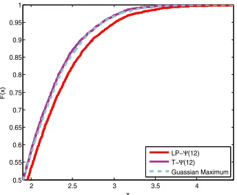
Figure 1. Comparison of the empirical cumulative distributions of LP-(ˆ 12), T-(ˆ 12)and the limiting cumulative distribution withn=180 andm=150. The plot is based on 5000 simulations.
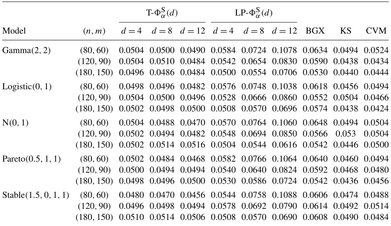
Next, we carry out 5000 simulations with nominal significance levelα=0.05 to calculate the empirical sizes of the proposed smooth testS
α(d). We denote with T-Sα(d)and LP-Sα(d), respectively, the tests based on the trigonometric series (2.7) and the LP polynomial series (2.6). The sample sizes (n, m) are taken to be (80,60), (120,90), (180,150), and d takes values 4,8,12. We compare the proposed smooth test with the testing procedure proposed by [5], the two-sample Kolmogorov–Smirnov test and the two-sample Cramér–von Mises test in five exam-ples when the data are generated from Gamma, Logistic, Gaussian, Pareto and Stable distribu-tions. The results are summarized in Table1, from which we see that among all the five examples considered, the empirical sizes of T-Sα(d)withd∈ {4,8,12}are close to 0.05. This highlights the robustness of the testing procedure T-Sα(d)with respect to the choice of the truncation pa-rameterd. Further, we note that the empirical sizes of LP-Sα(4)are comparable to those of BGX, while asd increases, the test LP-Sα(d)suffers from size distortion gradually. In fact, as pointed out by [38] and [4], when the Legendre polynomials series is used to construct the test statistic, the effectiveness of the corresponding test in each direction could be diluted ifd is too large. Nevertheless, the test based on the trigonometric series remains to be efficient asd increases and can be very powerful as we shall see later.
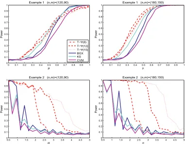
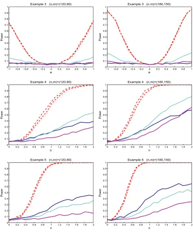
The power performance is evaluated through the following five examples. In each example, the result reported is based on 1000 simulations where samples sizes(n, m)are taken to be(120,90) and(180,150). Because of the distortion of empirical sizes of LP-Sα(d), we only compare the power of the trigonometric series based smooth test T-Sα(d)with that of the KS, CVM and BGX tests. The plots of power functions against different families of alternative distributions from Examples1–5are given in Figure2.
Example 1.
X:F =uniform(−1,1) versus Y :G=Gμ with densitygμ(x)=
1 2+2x
μ− |x|
Table 1. Comparison of empirical sizes with nominal significance levelα=0.05
T-Sα(d) LP-Sα(d)
Model (n, m) d=4 d=8 d=12 d=4 d=8 d=12 BGX KS CVM
Gamma(2,2) (80,60) 0.0504 0.0500 0.0490 0.0584 0.0724 0.1078 0.0634 0.0494 0.0524
(120,90) 0.0504 0.0510 0.0484 0.0542 0.0654 0.0830 0.0590 0.0438 0.0434
(180,150) 0.0496 0.0486 0.0484 0.0500 0.0554 0.0706 0.0530 0.0440 0.0444 Logistic(0,1) (80,60) 0.0498 0.0496 0.0482 0.0576 0.0748 0.1038 0.0618 0.0456 0.0494
(120,90) 0.0504 0.0500 0.0496 0.0528 0.0666 0.0860 0.0552 0.0504 0.0466
(180,150) 0.0502 0.0498 0.0500 0.0508 0.0570 0.0696 0.0574 0.0438 0.0424 N(0,1) (80,60) 0.0504 0.0488 0.0470 0.0570 0.0764 0.1060 0.0648 0.0494 0.0504
(120,90) 0.0502 0.0494 0.0482 0.0548 0.0694 0.0850 0.0566 0.053 0.0504
(180,150) 0.0502 0.0514 0.0516 0.0504 0.0544 0.0616 0.0542 0.0446 0.0500 Pareto(0.5,1,1) (80,60) 0.0502 0.0484 0.0468 0.0582 0.0766 0.1064 0.0640 0.0460 0.0494
(120,90) 0.0500 0.0494 0.0494 0.0540 0.0640 0.0824 0.0592 0.0468 0.0480
(180,150) 0.0498 0.0496 0.0500 0.0530 0.0586 0.0724 0.0542 0.0436 0.0456 Stable(1.5,0,1,1) (80,60) 0.0480 0.0470 0.0456 0.0544 0.0758 0.1088 0.0606 0.0474 0.0488
(120,90) 0.0496 0.0498 0.0494 0.0578 0.0692 0.0790 0.0614 0.0492 0.0514
(180,150) 0.0510 0.0514 0.0506 0.0508 0.0570 0.0690 0.0608 0.0490 0.0484
Example 2.
X:F=uniform(−1,1) versus Y :G=Gσ with densitygσ(x)=12
1+sin(2π σ x) (0.5≤σ≤5). Example 3.
X:F =lognormal(0,1) with densityf (x)=(2π )−1/2x−1exp−(logx)2/2 versus Y :G=Ga with densityga(x)=f (x)
1+asin(2πlogx) (−1≤a≤1).
Example 4.
X:F =uniform(0,1) versus
Y:G=Gc with densitygc(x)=exp
csin(5π x) (0≤c≤2). Example 5.
X:F =uniform(0,1) versus
Figure 2. Empirical powers for Examples1–5based on 1000 replications withα=0.05.
The first two examples are, respectively, Examples 5 and 6 in [21] which were designed to demonstrate the performance of the adaptive Neyman’s test proposed there. In Example1, when μ=0,Gμcoincides withF. For this family of alternatives index byμ, the strength of the local feature depends onμin the sense that the larger theμ, the stronger the local feature. As expected, the powers of all the tests considered grow withμand when sample sizes are large enough, the smooth tests T-Sα(d)uniformly outperform the others. Example2, on the other hand, is designed to test the global features with various frequencies. It can be seen from the second row in Figure2 that the test T-Sα(16)has the highest power that approaches to 1 rapidly asσdecreases to 0. The third example is from [28], wheregais a density and has the same moments asf0of any order.
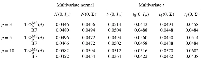
Table 2. Empirical size with significance levelα=0.05
Multivariate normal Multivariatet
N (0, Ip) N (0, ) t4(0, Ip) t8(0, Ip) t4(0, ) t8(0, )
p=3 T-MSα (d) 0.0446 0.0456 0.0514 0.0442 0.0494 0.0458 BF 0.0480 0.0494 0.0504 0.0488 0.0448 0.0484
p=5 T-MSα (d) 0.0496 0.0472 0.0494 0.0560 0.0450 0.0514 BF 0.0466 0.0472 0.0502 0.0458 0.0488 0.0484
p=10 T-MSα (d) 0.0582 0.0594 0.0512 0.0516 0.0570 0.0602 BF 0.0422 0.0454 0.0364 0.0422 0.0482 0.0438
5.2. Multivariate case
The computation of the proposed multivariate smooth test and the critical value requires to find optimal directionsuˆmaxanduˆMBmaxon the unit sphereSp−1that maximize non-smooth objective
functions (3.3) and (3.6), respectively. To solve these optimization problems, we convert the data into spherical coordinates and employ the Nelder-Mead algorithm. As a trade-off between the power and the computational feasibility of the test, we keep the value ofd fixed at 4.
Similar to the univariate case, we first carry out 5000 simulations with nominal significance levelα=0.05 to calculate the empirical sizes of the proposed test T-MSα (d)with trigonometric series. For eachp∈ {3,5,10}, the data are generated from multivariate normal andt-distributions with different degrees of freedom (4 and 8) and covariance structures (Ipand). Sample sizes (n, m) are taken to be (180,160). We summarize the results in Table 2, comparing with the method proposed by [1], which will be referred as the BF test. From Table2we see that when p=3,5, both methods have an empirical size fairly close to 0.05; whenp=10, the empirical size of the proposed smooth test increases since the optimization over the unit sphere becomes more challenging, while the empirical size of the BF test is typically smaller than the nominal level.
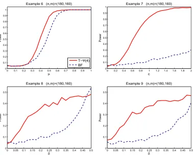
The power performance of the multivariate smooth test is evaluated through Examples6–9. The first two are multivariate versions of Examples1 and4, which demonstrate, respectively, the alternations with local feature and high frequency. The last two examples are designed to examine a rotation effect in the alternations. In each one, the power reported is based on 1000 simulations where samples sizes(n, m)are taken to be(180,160). Again, we compare the power of the trigonometric series based smooth test T-Sα(d)with that of the BF test. The power curve are depicted in Figure3.
Example 6.
X=(X1, X2, X3), X1, X2 i.i.d.
∼ uniform(−1,1), X3=0.3X1+0.7X2 versus
Y =(Y1, Y2, Y3), Y1, Y2 i.i.d.
∼ gμ(x)= 1 2+2x
μ− |x|
Figure 3. Empirical powers for Examples6–9based on 1000 replications withα=0.05.
Example 7.
X=(X1, X2, X3), X1, X2 i.i.d.
∼ uniform(0,1), X3=0.3X1+0.7X2 versus
Y =(Y1, Y2, Y3), Y1, Y2 i.i.d.
∼ gc(x)=exp
csin(5π x) (0≤c≤2), Y3=0.3Y1+0.7Y2.
Example 8.
X∼N(0, I5) versus Y =AZ, Z∼N(0, I5),
where
A=
A0 0
0 I3
, A0=
√
1−δ √δ √
δ √1−δ
Example 9.
X∼t4(0, I5) versus Y=AZ, Z∼t4(0, I5),
where
A=
A0 0
0 I3
, A0=
√
1−δ √δ √
δ √1−δ
(0≤δ≤0.5).
Figure3shows that the proposed smooth test uniformly outperforms the BF test in all the ex-amples in terms of power. Since we are using trigonometric series, the test is powerful especially if the data contains high frequency components (Example7), which is difficult to be detected by the BF test.
6. Discussion
We introduced in this paper a smooth test for the equality of two unknown distributions, which is shown to maintain the pre-specified significance level asymptotically. Moreover, it was shown theoretically and numerically that the test is especially powerful in detecting local features or high-frequency components.
The proposed procedure depends on a user-specific parameterd, which is the number of or-thogonal directions used to construct the test statistic. Theoretically, the size ofd is allowed to grow with n and can be as large aso(nc)for some 0< c <1. Since the optimal value ofd depends on how far the two unknown distributions deviate from each other, it is not possible to practically define an optimal choice ofd. As suggested by our numerical studies, d =10 is a reasonable choice when the sample sizes are in the order of 102, which leads a good compromise between the computational cost and the performance of the test. Alternatively, a data-driven approach based on a modification of Schwarz’s rule was proposed by [30], that is,dˆ=arg max1≤d≤D(n,m){T (d)−dlog(n+m)}for someD(n, m)→ ∞as min(n, m)→ ∞, whereT (d)is the test statistic using the first d orthonormal functions. This principal can be applied to the proposed testing procedure by settingD(n, m)to be some large value, say 20. Nevertheless, the optimal choice ofD(n, m)remains unclear.
The computation of the multivariate test statistic ˆmax(d)requires solving the optimization
problem with an2-norm constraint. To solve this problem when the dimensionp is relatively
small, we first convert the data into spherical coordinates and then use the Nelder-Mead algo-rithm. An interesting extension is to combine our method with the smoothing technique as in [29]. LetK:R→Rbe a symmetric, bounded density function. For a predetermined small number h=hn>0,ψˆu,kis approximated by a continuous functionψˆu,k,h=m−1
m
j=1ψk(Vˆj,hu ), where ˆ
Vj,hu =1 n
n
i=1 K
u(Yj−Xi) h
withK(t)=
t
−∞K(z) dz.
to the multiplier bootstrap statistic. Consequently, we can employ the gradient descent algo-rithm to solve the optimization for smooth functions. We leave a thorough comparison of various algorithms for different values ofpas an interesting problem for future research.
7. Proof of the main results
In this section, we prove Theorems4.1–4.3. Proofs of the lemmas and some additional technical arguments are given in Section8. Throughout this section, we writeN=n+mand useC and cto denote absolute positive constants, which may take different values at each occurrence. We writeab ifa is smaller than or equal tobup to an absolute positive constant, andabif ba.
7.1. Proof of Theorem
4.1
Recall thatG=(G1, . . . , Gd) is ad-dimensional standard Gaussian random vector, the dis-tribution of|G|∞ is absolute continuous so that P{|G|∞≥cα(d)} =α. Therefore, under the assumption thatd≤n∧m, the conclusion (4.8) follows from the following proposition immedi-ately.
Proposition 7.1. Assume that the conditions of Theorem4.1hold and let
γ0n=
(logn)7/8
n1/8 B0d, γ1n=
(logd)3/2 √
n B1d, γ2n=
logd
n B2d. (7.1) Then underH0:F =G,
sup t≥0
P(d)ˆ ≤t−P|G|∞≤tγ0n+√γ1n+√γ2n. (7.2)
The proof of Proposition7.1is provided in Section7.4.1.
7.2. Proof of Theorem
4.2
For thed-dimensional Gaussian random vectorG, applying the Borell–TIS (Borell–Tsirelson– Ibragimov–Sudakov) inequality [46] yields that for every t >0, P{|G|∞> E(|G|∞)+t} ≤ exp(−t2/2). By takingt=2 log(1/α), we get
cα(d)≤E
Letk∗=arg maxk∈[d]|θk|underH1d and assume without loss of generality thatθk∗>0. By (7.7) and (7.10) in the proof of Proposition7.1, we have
PHd
1
ˆ
> cα(d)
≥PHd
1
nm
N ψˆk∗> cα(d)
(7.4) =PHd
1 1 √ N N
j=1 ξj k∗+
nm
N (R1k∗+R2k∗) > cα(d)
,
whereξj k=√n/m{ψk(Vj)−ϑk}I{j ∈ [m]} +√m/nh1k(Xj−m)I{j ∈m+ [n]} for (j, k)∈ [N] × [d]withVj=F (Yj),ϑk=EHd
1{ψk(V )}andh1k(x)=EH1d(ψ
k(V )[I{V ≥F (x)} −V]). Note thatE{h1k(X)} =0 and thusE(ξj k)=0. LetE(t1, t2)be as in (7.12) fort1, t2>0 to be
specified. Putδ=t1B2d+t2B1d+ √
nm/N (θk∗−ϑk∗)+
2 log(1/α), then it follows from (7.3) and (7.4) that
PHd
1
ˆ
> cα(d)
≥PHd
1 1 √ N N
j=1 ξj k∗>
1+ 1 2 logd
2 logd+δ−
nm N θk∗
−PE(t1, t2)c
≥PHd
1 1 √ N N
j=1 ξj k∗>
1 2 logd −
ε 2
2 logd+δ
−PE(t1, t2)c
.
In particular, takingt1=t1n(d)n−1/2 √
logd andt2=t2n(d)n−1/2logd implies by (7.16) thatP{E(t1, t2)c} →0 asd→ ∞. Further, by (8.8) and the conditions of the theorem, we have δ=o(√logd). Consequently, asd→ ∞,
PHd
1
ˆ
> cα(d)
≥1−PHd
1 1 √ N N
j=1
ξj k∗≤ − ε 2
logd
−PE(t1, t2)c
→1.
This completes the proof of Theorem4.2.
7.3. Proof of Theorem
4.3
We first introduce two propositions describing the limiting null properties of the multivariate smooth and multiplier bootstrap statistics used to construct the test. The conclusion of Theo-rem4.3follows immediately.
The first proposition characterizes the non-asymptotic behavior of the multivariate smooth statisticˆmax(d)which involves the supremum of a centered Gaussian process. LetF=Fdpbe
Proposition 7.2. Suppose that Assumptions4.1and4.3hold.Then there exists a centered,tight Gaussian processGindexed byFsuch that under the null hypothesisH0:F=G,
sup t≥0
Pˆmax(d)≤t
−PGF≤t≤Cn−c, (7.5)
whereC andcare positive constants depending only onc0, c1, C0andC1.
Proposition7.2implies that the “limiting” distribution ofˆmaxdepends on unknown the
co-variance structure given in (3.5). To compute a critical value, we suggest to use multiplier boot-strapping as described in Section3.2. The following result, which can be regarded as a multiplier central limit theorem, provides the theoretical justification of its validity. In fact, the construc-tion of the multiplier bootstrap statisticˆmaxMB(d)involves the use of artificial random numbers to simulate a process, the supremum of which is (asymptotically) equally distributed asGF according to Proposition7.3below.
Proposition 7.3. Suppose that Assumptions 4.1 and 4.3 hold. Then with probability at least 1−3n−1,
sup t≥0
Pe
ˆ
maxMB(d)≤t−PGF≤t≤Cn−c (7.6)
forGas defined in Proposition 7.2,where C and care positive constants depending only on c0, c1, C0andC1.
Proofs of the above two propositions are given in Section7.4.
7.4. Proof of Propositions
7.1–7.3
7.4.1. Proof of Proposition7.1
For everyk∈ [d], it follows from (2.2) and Taylor expansion that 1
m m
j=1
ψk(Vˆj)= 1 m
m
j=1
ψk(Vj)+ 1 m
m
j=1
ψk(Vj)(Vˆj−Vj)+ 1 2m
m
j=1
ψk(ξj)(Vˆj−Vj)2
(7.7) = 1
m m
j=1
ψk(Vj)+ 1 nm
n
i=1
m
j=1 ψk(Vj)
I (Xi≤Yj)−F (Yj)
+R1k,
where R1k :=(2m)−1
m
j=1ψk(ζj)(Vˆj −Vj)2 and ζj is a random variable lying between ˆ
Vj and Vj. It is straightforward to see that R1k ≤ 12ψk∞max1≤j≤m(Vˆj −Vj)2. A di-rect consequence of the Dvoretzky–Kiefer–Wolfwitz inequality [36], that is, for every t >0, P{√nsupx|Fn(x)−F (x)|> t} ≤2 exp(−2t2), is that
P
n max
1≤k≤d|R1k|/
ψk∞> t
Let hk(x, y)=ψk(F (y)){I (x ≤y)−F (y)} for x, y ∈R be a kernel function R×R→
R. Then the second addend on the right-hand side of (7.7) can be written as Un,m(k)= (nm)−1ni=1mj=1hk(Xi, Yj)withE{hk(X, Y )} =0. Observer thatUn,m(k)is a two-sample U-statistic with a bounded kernelhksatisfyingbk:= hk∞≤ ψk∞and
σk2:=Ehk(X, Y )2
=EV−V2ψk(V )2≤ψk2∞/4. (7.9) Leth1k(x)=EHd
0{hk(X, Y )|X=x}andh2k(y)=EH0d{hk(X, Y )|Y =y}be the first order pro-jections of the kernelhkunderH0d. SinceXandY are independent and underH0,V =F (Y )=d
Unif(0,1)underH0, we haveh2k≡0 and
h1k(x)=E
ψk(V )IV ≥F (x)−V=
1
F (x)
ψk(v) dv−
1
0
vψk(v) dv= −ψk
F (x).
Define random variablesUi=F (Xi)=dUnif(0,1)that are independent ofVj=F (Yj). Then, using the Hoeffding’s decomposition gives
Un,m(k)= − 1 n
n
i=1
ψk(Ui)+ 1 nm
n
i=1
m
j=1
h0k(Xi, Yj):= − 1 n
n
i=1
ψk(Ui)+R2k, (7.10)
whereh0k(x, y)=hk(x, y)−h1k(x)−h2k(y).
In view of (7.7) and (7.10), we introduce a new sequence of independent random vectors {ξj=(ξj1, . . . , ξj K)}Nj=1forN=n+m, defined by
ξj k=
√
n/mψk(Vj), 1≤j≤m, −√m/nψk(Uj−m) m+1≤j≤N.
(7.11)
Putψ=(ψ1, . . . , ψd),R1=(R11, . . . , R1d)andR2=(R21, . . . , R2d), such that
n mN
m
j=1
ψ(Vˆj)= 1 √
N N
j=1
ξj+
nm
N (R1+R2).
Recall that{ψ0≡1, ψ1, . . . , ψd}is a set of orthonormal functions andV =dUnif(0,1)underH0.
By (7.11), the covariance matrix ofN−1/2Nj=1ξj is equal toId. For anyt1, t2>0, define the event
E(t1, t2)=
d
k=1
√
m|R1k| ≤ψk∞t1
∩√m|R2k| ≤ψk∞t2
. (7.12)
UnderH0, we have for everyt >0, PH0
ˆ
(d)≤t =P max
1≤k≤d
n mN m
j=1 ψk(Vˆj)
≤t
=P max
1≤k≤d
1 √ N N
j=1 ξj k+
nm
N (R1k+R2k)
≤t
≤P max
1≤k≤d
1 √ N N
j=1 ξj k
≤t+
n
N(t1B2d+t2B1d)
+PE(t1, t2)c
,
whereBd(=1,2) are as in (4.1). To get rid of the absolute value in (7.13), a similar argument as in the proof of Theorem 1 in [10] gives
P
max
1≤k≤d
1 √ N N
j=1 ξj k
≤t =P max
1≤k≤2d 1 √
N N
j=1 ξj kext≤t
, (7.14)
where {ξextj }Nj=1 is a sequence of dilated random vectors taking values in R2d defined by ξextj =(ξjext1, . . . , ξj,ext2d) = (ξj,−ξj). In view of (7.14), we only need to focus on max1≤k≤dN−1/2Nj=1ξj kwithout losing generality.
Note thatξj k are bounded random variables satisfyingE(ξj k)=0 and |ξj k| ≤
n
mψk∞. Applying Lemmas 2.3 and 2.1 in [11], respectively, yields
sup t∈R P max
1≤k≤d 1 √
N N
j=1 ξj k≤t
−P
max
1≤k≤dGk≤t
{log(dn)}7/8 n1/8 Bd,
whereBd:= [E{max1≤k≤d|ψk(V )|3}]1/4≤B03d/4,G=(G1, . . . , Gd)=dN (0,Id)and for ev-eryε >0,
sup t∈R
Pmax
1≤k≤dGk−t
≤ε
≤4ε(1+2 logd).
The last two displays jointly imply
P max
1≤k≤d 1 √
N N
j=1
ξj k≤t+
n
N(t1B2d+t2B1d)
(7.15) ≤P
max
1≤k≤dGk≤t
+C
{log(dn)}7/8 n1/8 B
3/4
0d +(logd)
1/2(t
1B2d+t2B1d)
.
ForP{E(t1, t2)c}in (7.13), it follows from (7.8) and (8.3) in Lemma8.2that
PE(t1, t2)c
≤2 exp(−4t1n/
√ m)+
d
k=1
P√m|R2k|>ψk∞t2/2
(7.16)
exp(−4t1
√
n)+dexp(−ct2