Non-parametric maximum likelihood estimation of interval censored
failure time data subject to misclassification
Andrew C. Titman
September 30, 2016
Abstract
The paper considers non-parametric maximum likelihood estimation of the failure time distribution
for interval censored data subject to misclassification. Such data can arise from two types of observation
scheme; either where observations continue until the first positive test result or where tests continue
regardless of the test results. In the former case, the misclassification probabilities must be known,
whereas in the latter case joint estimation of the event-time distribution and misclassification
proba-bilities is possible. The regions for which the maximum likelihood estimate can only have support are
derived. Algorithms for computing the maximum likelihood estimate are investigated and it is shown
that algorithms appropriate for computing non-parametric mixing distributions perform better than an
iterative convex minorant algorithm in terms of time to absolute convergence. A profile likelihood
ap-proach is proposed for joint estimation. The methods are illustrated on a data set relating to the onset
of cardiac allograft vasculopathy in post-heart-transplantation patients.
1
Introduction
Interval censored time-to-event data is commonly encountered in applications in which continual monitoring
is not possible and instead the status of a subject, for instance whether they have developed a disease, is
only known at intermittent observation or examination times. It is usually assumed that the status of the
This is the peer reviewed version of the following article:
Titman, A.C. (2016) Non-parametric maximum likelihood estimation of interval censored failure time data subject to mis-classificationStatistics and Computing. DOI:10.1007/s11222-016-9705-7,
process can be determined with complete accuracy at each of these examination times. However, in many
medical applications where the event of interest is onset of a disease or onset of infection, diagnosis may be
subject to classification error.
Time-to-event data subject to misclassification error has been considered previously. Espeland et al
(1989) analyzed data relating to the diagnosis of onset of puberty in adolescents and considered a discrete
time model where events could occur within ‘sub epochs’ of ‘epochs’ for which the incidence rate was assumed
constant. They developed an EM algorithm that allowed for estimation of the underlying incidence rates
and error probabilities. Balasubramanian and Lagakos (2003) considered estimation for a general continuous
time model, but ensured identifiability by fixing the increments in the failure time distribution to be equal
between some time points. Fully non-parametric estimation of the failure time distribution F(t) has been considered in the case of current status (or Type I interval censored) survival data subject to misclassification
of outcomes (McKeown and Jewell (2010); Sal y Rosas and Hughes (2011)). In that case, since each subject
is observed precisely once, the misclassification probabilities must be knowna prioriin order to estimate the
survivor distribution.
The purpose of this paper is to develop methods for fully non-parametric estimation of the failure time
distribution, F(t), for general (or mixed case) interval censored data subject to classification error, by extending existing methods for standard interval censored survival data. Two observation schemes are
considered. In the first scenario, observations may be assumed to persist only until the first observed failure.
Such an observation scheme has been considered in a discrete-time setting by Richardson and Hughes (2000)
where patients were assessed based on an imperfect diagnostic test, with known error probabilities, repeatedly
until their first positive test at which point they were treated and hence left the study. In this case, the
misclassification probabilities must be known in order to estimateF(t).
However, a second scenario is also considered where it is assumed that examinations of a subject continue
to occur regardless of whether a positive result has been observed. This type of observation has been
considered both for interval censored survival data without misclassification (Betensky et al, 2001; Zhu et al,
2008) and for misclassified data (Espeland et al, 1989). Such data may arise in studies where there are several
outcomes of interest. In this case methods to jointly estimate F(t) and the misclassification probabilities, which can be constant or depend parametrically on time, are considered.
The remainder of the paper is organized as follows. Section 2 formalizes the problem and
character-izes the non-parametric maximum likelihood estimate (NPMLE), Section 3 discusses computation of the
a numerical study and Section 6 gives an illustrative example based on data from post-heart-transplantation
patients. The paper concludes with a discussion of potential model extensions.
2
Non-parametric Maximum Likelihood Estimate
Consider failure timesTj ∼F(t) for subjectsj= 1, . . . , n, indirectly observed through a series of observations Yj= (Y1j, . . . , Ynjj) at timesXj = (X1j, . . . , Xnjj) whereYij is a binary random variable such that
P(Yij = 1|Xij < Tj) =α(Xij;θ)
and
P(Yij= 0|Xij ≥Tj) =β(Xij;θ).
At each observation time, Yij is the outcome of an imperfect diagnostic test where the functions α(x;θ)
and β(x;θ) represent the probabilities of a false positive and false negative result, respectively, and may depend on the age of the process, x. It is assumed thatα(x;θ) andβ(x;θ) are known functions satisfying 0≤α(x;θ)<1, 0≤β(x;θ)<1 and 0≤α(x;θ) +β(x;θ)<1 for all θ ∈Θ andx > 0. The observation timesXij are potentially random, but are assumed to be generated from a process that is non-informative
forF andθ, as defined by Gr¨uger et al (1991).
Interest lies in estimatingF and possibly alsoθ.When observations stop at the first failure time,α(x;θ) andβ(x;θ) must be fully specified. However, if observations persist after a first positive result thenθ can also be estimated.
In the simplest case, the diagnostic test performed at each observation time would be assumed to have
fixed sensitivity, (1−α), and specificity (1−β). A convenient way to parameterize this is through a logistic transformation such that α(x;θ) = (1 + exp(−θ1))−1 and β(x;θ) = (1 + exp(−θ2))−1 for θ = (θ1, θ2).
Alternatively if, as in Espeland et al (1989), the test accuracy is considered age-dependent, this could be
represented by
logit{α(x;θ)}=
θ1 ifx < τ1
θ1+θ2 ifτ1≤x < τ2
..
. ...
θ1+θm x≥τK−1,
for fixed cut-points 0< τ1< . . . < τK−1, with a similar expression forβ(x;θ), implying that the sensitivity
Assuming the observation times, Xj are non-informative, the likelihood with respect to F for a single
subjectj can be expressed as
Lj = nj+1
X
i=1
{F(Xij+)−F(Xi−1j−)} × i−1
Y
k=1
α(Xkj;θ)Ykj(1−α(Xkj;θ))1−Ykj ×
nj
Y
k=i
β(Xkj;θ)1−Ykj(1−β(Xkj;θ))Ykj
whereX0j= 0 andXnj+1j=∞andF(∞) = 1. Note that in the case whereα≡β ≡0, such that there is no classification error, the expression reduces to the standard expression for interval censored survival data,
Lj = nj+1
X
i=1
{F(Xij+)−F(Xi−1j−)}I(Yij = 1, Yi−1j= 0)
= {F(Rj+)−F(Lj−)}.
whereY0j= 0 and Ynj+1j= 1 and Rj= mini({Xij0 :Yij0 = 1, j
0 =j} ∪ {∞}) andL
j= maxi({Xij0 :Yij0 =
0, j0=j} ∪ {∞}).
2.1
Support of the NPMLE
Under standard interval censored survival data, the non-parametric maximum likelihood estimate (NPMLE)
is only uniquely defined up to increments of mass within semi-closed intervals between unique observation
times (Turnbull, 1976; Ng, 2002). The NPMLE for misclassified survival data also has this property and it
is only the determination of the particular intervals of support which differs.
Initially assume thatα(x;θ)>0, β(x;θ)>0 for allx≥0 and that examination times are generated from a continuous distribution such that there are no tied observation times with probability 1. For notational
convenience in the proof below the dependence of α and β on x and θ is suppressed, but the argument remains valid for non-constant error probabilities.
Let L = {0} ∪ {Xij : Yij = 0} and R = {Xij : Yij = 1} ∪ {∞} denote the sets of observation times
corresponding to negative and positive test results, respectively.
A further set can be constructed consisting of disjoint intervals whose left and right end points lie in the
setsL andRrespectively and which do not contain any members ofL orR. Let{Qi := (li, ri],1≤i≤I}
be those intervals, wherel1< r1< l2< r2< . . . < lI < rI ≤ ∞andQ=∪iQi. Theorem 1
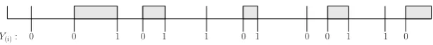
Y(i): 0 0 1 0 1 1 0 1 0 0 1 1 0
Figure 1: Example of the (shaded) support regions of the NPMLE for a particular set of pooled observations
Y(i)corresponding to the ordered observation timesX(i) Proof
LetX(i)denote theith ordered observation time from the pooled set of observation times across all subjects,
with corresponding observation Y(i). Suppose the NPMLE, ˆF, increases by > 0 between times X(i)
and X(i+1) corresponding to observations Y(i) and Y(i+1), where Y(i) = 1. Construct ˜F to be identical
to ˆF except that the increment on (X(i), X(i+1)] is set to zero and the increment on (X(i∗), X(i∗+1)] is
increased from π0 to π0+, where i∗ = arg max
j {j : j < i, Y(j) = 0, Y(j+1) = 1}. The likelihood under
ˆ
F and ˜F is equal for all subjects except individuals observed at time points X(i∗+1), . . . , X(i). For each
of these subjects, assuming they are observed exactly once in [X(i∗+1), X(i)], their likelihood contributions
are of the form L( ˆF) =C+K(π0(1−β) +α) and L( ˜F) = C+K(π0+)(1−β), for some C, K > 0.
Hence L( ˜F)−L( ˆF) = K(1−β −α) > 0, since α+β < 1, and therefore ˆF cannot be the MLE. If there are subjects observedm > 1 times within [X(i∗+1), X(i)] thenL( ˆF) =C+K(π0(1−β) +α)m and
L( ˜F) =C+K(π0+)m(1−β)m andL( ˜F)> L( ˆF) providedα+β <1.
Similarly, suppose the NPMLE, ˆF, increases by > 0 between times X(i) and X(i+1) corresponding
to observations Y(i) and Y(i+1), where Y(i+1) = 0. Construct ˜F to be identical to ˆF except the increment
on (X(i), X(i+1)] is set to zero and the increment on (X(i∗), X(i∗+1)] is increased from π0 to π0+, where
i∗ = arg min
j {j : j > i, Y(j) = 0, Y(j+1) = 1}. The likelihood contributions under ˆF and ˜F are equal
for all subjects except individuals observed at time points X(i+1), . . . , X(i∗+1). For each of these subjects,
assuming they are observed exactly once in [X(i+1), X(i∗+1)] their likelihood contributions are of the form
L( ˆF) =C+K(π0(1−β) +α) whileL( ˜F) =C+K(π0+(1−β), for someC, K >0. HenceL( ˜F)−L( ˆF) =
K(1−β−α)>0 sinceα+β <1, and therefore ˆF cannot be the MLE. Again, a similar argument follows for subjects observedm >1 times within [X(i+1), X(i∗+1)].
Figure 1 illustrates the implied support regions for a particular set of pooled observations ordered by
observation time.
individual’s failure time can be determined to have occurred before the first positive observation. Define
Xj−= inf({Xij0 :Yij0 = 1, j0=j} ∪ {∞}) forj= 1, . . . , nand letL−=∪j{Xij0 :Yij0 = 0, Xij0 < Xj−, j0=
j} ∪ {0}andR−=∪j{Xij0 :Xij0 =X− j , j
0 =j} ∪ {∞}.The set of support,Q, is then constructed from the
disjoint closed setsL− andR−.
If β(x;θ) ≡0, an individual’s failure time can be determined to have occurred after the last observed 0. Define Xj+ = sup({0} ∪ {Xij0 : Yij0 = 0, j0 =j}) and letL+ =∪j{Xij0 : Xij0 =Xj+, j0 = j}{0} and R+=∪
j{Xij0 :Yij0 = 1, Xij0 > Xj+, j0=j} ∪ {∞}. The set of supportQis then constructed from L+ and R+.
Ifα(x;θ)6≡0 andβ(x;θ)6≡0 but are equal to zero for some observation times, defineXj−= inf({Xij0 :
Yij0 = 1, α(Xij0;θ) = 0, j0 =j} ∪ {∞}) andXj+ = sup({0} ∪ {Xij0 : Yij0 = 0, β(Xij0;θ) = 0, j0 =j}) and L± = ∪j{Xij0 : Yij0 = 0, X+
j ≤ Xij0 < X− j , j
0 = j} ∪ {0} and R± = ∪
j{Xij0 : Yij0 = 1, X+
j < Xij0 ≤
Xj−, j0 =j} ∪ {∞}. Again the set of supportQis constructed fromL± andR±.
Whenα(x;θ)≡β(x;θ)≡0, the data are standard interval censored and the support set is defined as in Turnbull (1976) in the case where there is no truncation.
The above assumes the observation times are unique. If there are ties we can define X(i) to be the
ith ordered unique observation time and an analogous argument can be applied to show that a necessary condition for the NPMLE to increase on (X(i), X(i+1)] is that at least one observed state at timeX(i)must
be 0 and at least one observed state at timeX(i+1) must be 1.
2.2
Optimality conditions
B¨ohning et al (1996) noted the relationship between the non-parametric estimates of the survivor function
for interval censored data and the NPMLE of a mixing distribution. This relationship also exists in the case
of misclassified failure time data. Again assuming theXij are non-informative, the likelihood with respect
toF for a single individual can also be expressed as
Lj =
Z ∞
0 nj
Y
i=1
P(Yij|Xij, Tj=t)dF(t),
where the unobserved failure timeTj acts as a mixing variable.
Having established the support of the NPMLE in Section 2.1, the likelihood can be expressed in terms
of a finite mixture. Let
represent the joint probability of subject j’s outcome vector Yj given observation times Xj and that the
failure time for subjectjoccurs within theith support region,Qi= (li, ri]. Note thatγij(α, β) depends on the
full classification probability functionsα(x;θ) andβ(x;θ) but this dependence is suppressed for notational convenience. Denote the probability that the failure occurs in theith support region asπi=F(ri)−F(li−)
withπ= (π1, . . . , πI) then the likelihood for the data can be written as
L(π) =
n Y j=1 I X i=1
γij(α, β)πi.
LetSbe theI×nmatrix with (i, j) entry
dij(π) =
γij(α, β)
PI
k=1γik(α, β)πk
,
the first and second derivatives of the log-likelihood can be expressed as∇logL= (S1)0 and∇2logL=SS0
respectively, hence the Hessian is positive-semi-definite and logLis concave.
In general,γij(α, β) can be computed by considering which of subjectj’s observations,Yj, would be false
positives, true positives, false negatives and true negatives given the failure occurred in (li, ri] and computing
the relevant probability at the corresponding event times. Hence the general expression is of the form
γij(α, β) = n Y j=1 nj Y k=1
α(Xkj;θ)YkjI(Xkj<li−1)(1−α(Xkj;θ))(1−Ykj)I(Xkj<li−1) ×β(Xkj;θ)(1−Ykj)I(Xkj≥ri)(1−β(Xkj;θ))YkjI(Xkj≥ri).
However, in the special case where the misclassification probabilities are time constant it is only necessary
to count the number of false and true negatives and positives, so that the expression can be simplified to
γij(α, β) =αn −
1j(li−1)(1−α)n−0j(li−1)βn+0j(ri)(1−β)n+1j(ri) (2.1) where
n−1j(t) =
nj
X
k=1
YkjI(Xkj< t), n+1j(t) =
Pnj
k=1YkjI(Xkj≥t),
n−0j(t) =
nj
X
k=1
(1−Ykj)I(Xkj< t), n+0j(t) =
Pnj
k=1(1−Ykj)I(Xkj≥t).
Finally, in the case where there is no classification error, such thatα=β= 0 and meaning a subject’s failure time can be bounded by (Lj, Rj], the expression reduces to
γij(0,0) =I((li, ri]⊆(Lj, Rj]).
This expression can be derived from (2.1) by adopting the convention that 00 = 1 and noting that when
The NPMLE ofFcan be obtained by considering the constrained maximization problem maxπlog(L(π))
subject to PI
i=1πi = 1 and πi ≥0 for alli. The Kuhn-Tucker conditions for π to be the NPMLE relate
to the directional derivatives. The directional derivative of L(π) fromπ to a mixing distribution with all mass in the interval (li, ri] is given bydi(π) =P
n
j=1dij(π)−n. The Kuhn-Tucker conditions for optimality
can then be expressed as maxidi(θ) = 0. The equivalence of maximizing the likelihood with minimizing
the largest directional derivative and finding the solution with maxidi(θ) = 0 can also be shown by using a
fundamental theorem of mixture estimation in Lindsay (1983), which is analogous to the general equivalence
theorem of optimal design.
3
Computation
Initial proposals for algorithms for finding the NPMLE both in the case of interval censored survival data
(Turnbull, 1976) and also in the case of non-parametric mixing distributions (Laird, 1978), were based
upon EM algorithms. However, in each case other algorithms have been devised with substantially better
properties. This section considers applying two of the best performing algorithms to the problem of finding
the NPMLE for misclassified data.
3.1
Iterative convex minorant algorithm
The best performing algorithms for computing the NPMLE for interval censored survival data are the
iterative convex minorant (ICM) algorithm (Jongbloed, 1998) or hybrid ICM-EM algorithm (Wellner and
Zhan, 1997). In principle, an ICM type algorithm could also be used for misclassified survival data.
The ICM approach parameterizes by Fi where πi =Fi−Fi−1 and uses a quadratic function about Fi
based on its gradient and approximate Hessian (taken as the diagonal of the full Hessian) and maximizes
this quadratic form with respect to monotonicity constraints on F. Under this parameterization, the first derivatives of the log-likelihood have the form
gi=
∂logL ∂Fi
=X
k
γik−γi+1k
Lk
and the diagonal elements of the Hessian have the form
Hii=−
∂2logL
∂F2 i
=X
k
(γik−γi+1k)2
L2 k
.
isotonic regression problem
minX
i
Hii( ˆF−F˜ (s)
i −
gi
Hii
)2 (3.1)
subject to monotonicity constraints on ˆF. This can be achieved by using the pool-adjacent-violators (PAV) algorithm (Barlow et al, 1972).
However to guarantee convergence, it is necessary to include a line search step where ˜F(s+1) is taken to be the point on the line ˜F(s)+ ( ˆF−F˜(s))d,d∈(0,1] for which the likelihood is maximized. In practice, as
suggested by Jongbloed (1998), the line search only needs to be applied if taking the step lengthd= 1, i.e. applying ˜F(s+1)= ˆF does not result in an increase in the likelihood or increases the likelihood by less than some specified threshold.
The effectiveness of (3.1) as a quasi-Newton step and hence the effectiveness of ICM as a whole, depends
on the extent to which the full Hessian can be approximated by its diagonal. For standard interval censored
data the approximation is usually quite effective since each subject’s failure time can be observed to have
only occurred in a small proportion of the support regions. In contrast for misclassified data, with imperfect
sensitivity and specificity, no support regions can be ruled out for any subject. The effectiveness of a diagonal
approximation will depend on the error probabilitiesαandβ, with better performance expected when these are smaller.
3.2
Constrained Newton algorithm
Given the representation as a non-parametric mixture problem, an alternative approach to take is to use an
algorithm appropriate for finding the NPMLE of a mixing distribution. Several such algorithms exist, for
instance the vertex exchange method (B¨ohning (1985)), the intra-simplex direction method (Lesperance and
Kalbfleisch (1992)) and the constrained Newton method of Wang (2007). Here an adapted version of this
latter algorithm is proposed.
The main idea behind the constrained Newton algorithm is to use the optimality condition based upon
the directional derivatives, to determine the best locations to add new support points or regions. Specifically
it seeks the maximum, or maxima, of the directional derivatives, with respect to the mixing parameter π
and proposes these points as additions to the finite mixture.
The constrained Newton algorithm can be difficult to implement for a general non-parametric mixture
where as it requires a line search over the continuous space ofπto find the maxima. However, the problem is simplified for the case of misclassified interval censored data, as the support reduction step ensures that
The proposed algorithm involves collecting a set of support intervals I ⊆Q, where πi >0 for all i∈ I
and πi = 0 for all i 6∈ I. Set s = 0 and an initial feasible π(s) implying a support set I(s), such that
logL(π(s))>−∞.
1. Find the set I∗ of i ∈ I(s) such that d
i(π(s)) > di−1(π(s)) and di(π(s)) > di+1(π(s)) where, by
convention,d0(π(s)) =dI+1(π(s)) = 0.If maxidi(π(s)) = 0 stop.
2. SetI+=I ∪ I∗.Computeπ(s+1) by performing one constrained Newton iteration.
3. Discard all points inI+ with zero entries inπ(s+1) to obtainI(s+1). Sets=:s+ 1 and return to 1.
Step 2 of the algorithm involves maximizing a quadratic approximation to logL(π) in a neighbourhood ofπ(s). Wang (2007) shows that this is equivalent to solving min
π∗||Sπ∗−2||2subject toπ∗ 0
1= 1, π∗ i ≥0
for alli∈ I+, which in turn can be solved using the non-negative least squares (NNLS) algorithm (Lawson
and Hanson (1974)).
A simplified procedure, which retains all possible support points forπat each iteration of the algorithm,
would also be effective but somewhat slower due to requiring a larger NNLS problem to be solved at each
iteration.
In Section 5 the performance of the constrained Newton algorithm is compared with the ICM algorithm.
3.3
Semi-parametric estimation
In the scenario in which observation continues after the first observed failure, there is scope for joint
estima-tion ofF and the misclassification probabilitiesα(x;θ) andβ(x;θ). In this case the model can be expressed as a semi-parametric mixture, where the mixture distribution - defined throughF - is non-parametric, but there are additional parameters determining the response conditional on the mixture component.
Provided α(x;θ), β(x;θ)>0 and α(x;θ) +β(x;θ)<1 for allx > 0 andθ ∈Θ, the potential support points of F will remain fixed. This ensures that the profile likelihood is differentiable with respect to θ, provided α(x;θ) andβ(x;θ) are themselves differentiable. The maximum likelihood estimate can be found by maximizing the profile log-likelihood
pl(θ) =l(θ,π(θ))ˆ .
Clearly, the profile likelihood can be computed by applying the algorithm for non-parametric estimation for
used to maximize the profile likelihood, using finite-difference approximations to evaluate
∂pl(θ)
∂θ =
∂l(θ,π)
∂θ
π= ˆπ(θ)
.
4
Estimates of uncertainty
Estimation of standard errors or the construction of confidence intervals forF is not straightforward since, in common with other NPMLE for mixing distributions or interval censored data standardn1/2asymptotics do
not apply and instead the estimator converges at a slower rate (van de Geer, 2003). In the context of current
status data, some progress has been made in developing asymptotic theory. For instance, if the observation
times are random and generated from a continuous distribution, the convergence rate of the NPMLE is
n1/3 (Groeneboom and Wellner, 1992). Banerjee and Wellner (2001, 2005) derive the limiting form of
the likelihood ratio and Tang et al (2012) have developed an adaptive inference procedure suitable when
the nature of the sampling times distribution, and hence the convergence rate, is unknown. However, these
results are not easily extendable either to general (mixed case) interval censored data or to misclassified data.
Abrevaya and Huang (2005) showed that standard non-parametric bootstrap approaches are not consistent
for estimators withn1/3convergence implying that the standard non-parametric bootstrap is unlikely to be
consistent for misclassified survival data.
Possible approaches to quantifying the uncertainty in ˆF could involve either a parametric bootstrap, though this requires estimation of the inspection process, subsampling (Politis and Romano, 1994) ifn1/3
convergence can be assumed, or the use of a smoothed bootstrap (Sen and Xu, 2015). If the distribution of
examination times can be assumed to have finite support, then standardn1/2 asymptotics will apply, but
may nevertheless have poor performance in finite samples (Maathuis and Hudgens (2011)).
For the semi-parametric case, if interest is in estimation of the parametersθthat determineαandβ, with
F as a nuisance parameter, then through direct application of results from Murphy and van der Vaart (1997), profile likelihood ratio based confidence intervals can be obtained. An asymptotic 100(1−ν)% confidence region forθ can be found by taking
{θ: 2{l( ˆθ,Fˆθˆ)−l(θ,Fˆθ)} ≤χ2|θ|(ν)}. (4.1)
A confidence interval for an individual component, θk of θ can be found in a similar way by inverting a
profile likelihood ratio test with respect toθk, which profiles out the other components ofθ as well asF.
Alternatively, standard errors can be obtained by computing the Hessian of the profile likelihood through a
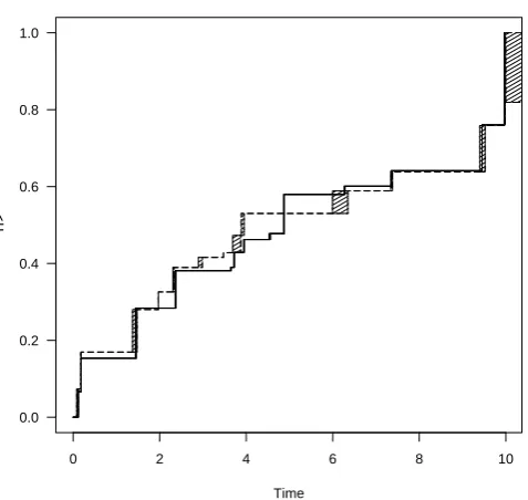
0 2 4 6 8 10 0.0
0.2 0.4 0.6 0.8 1.0
Time
[image:12.595.183.422.96.322.2]F^
Figure 2: Comparison of the NPMLE for the misclassified data (solid line and solid shading) and the NPMLE
for the interval censored data (dashed line and cross hatched shading).
5
Numerical Investigation
To illustrate the differences between the estimation of the NPMLE for interval censored data and the NPMLE
for misclassified data a dataset of n = 100 subjects is simulated. The sampling times are random with independent gap times distributed U(0,2) up to a fixed administrative censoring time at t= 10. From the true classifications, I(Ti < Xij), standard interval censored survival data, consisting of pairs (Lj, Rj], can
be obtained. In addition misclassified data, taking the misclassification probabilities to be fixed in time as
α= 0.05 andβ= 0.1, is generated. The failure time distribution is estimated, first assuming (α, β) are fixed and known and second by jointly estimating (α, β). Figure 2 shows the estimates for a particular simulated dataset.
Applying the ICM and proposed constrained Newton algorithms for αand β at their true values, the convergence of the constrained Newton algorithm was considerably faster than that of ICM. Convergence,
assessed based upon a criterion of maxdi<1×10⁻⁸, was reached in 27 iterations using constrained Newton
compared to 281 iterations with ICM. This also corresponded to a CPU time of 0.28s for constrained Newton
Table 1: Proportion of simulated likelihood ratio statistics above nominalχ22upper quantiles
Nominal upper quantile
n 0.5 0.2 0.1 0.05 0.01 100 0.562 0.256 0.138 0.070 0.014
500 0.536 0.255 0.134 0.067 0.016
of the PAV and NNLS algorithms. Here, there should be reasonable comparability since in each case Fortran
routines ported intoRvia the packagesIsoandnnls, respectively. Similarly, in each case the starting point
was chosen such that all mass inF was in the single support regionj for whichPn
i=1γij was maximized.
The number of increments of the NPMLE is similar for the interval censored and the misclassified data.
However, the regions of support are typically much narrower for the misclassified data because they are
always bounded by consecutive unique ordered sampling times.
Over 1000 samples of n= 100, the median number of increments of the NPMLE was 15 for both the standard interval censored data and the misclassified data. The mean width of support regions, excluding
those bounded by∞, was 0.07 for standard interval censored data and 0.01 for the misclassified data.
Table 1 compares the distribution of the profile likelihood ratio statistic, 2{l( ˆθ,Fˆθˆ)−l(θ0,Fˆθ0)}, testing
a null hypothesis that θ0 = (α, β) = (0.05,0.1), across 1000 samples of n = 100 and n = 500 against
the asymptoticχ2
2 distribution. This shows that the likelihood ratio test is slightly anti-conservative which
implies that constructed confidence regions using (4.1) would tend to have lower than nominal coverage.
6
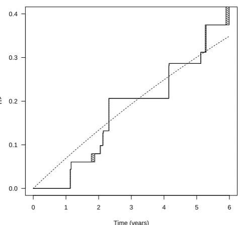
Example: Onset of Cardiac Allograft Vasculopathy
As an illustrative example, an analysis of data on the time of onset of cardiac allograft vasculopathy (CAV)
among post-heart-transplantation patients is presented. CAV is the narrowing of arteries of the transplanted
heart and is asymptomatic in its early stages. Patients are diagnosed through angiographic surveillance which
is known to misdiagnose in some cases.
The data consist of the apparent presence or absence of CAV at a series of patient specific examination
times. Diagnoses were made on the basis of 1304 angiograms taken from 562 patients in their first 6 years
donated organs are healthy such that the patients will be CAV free at the time of transplantation.
Observations continue to take place after the first positive diagnosis so it is possible to jointly estimate
the time-to-onset distribution as well as the false positive and false negative rates of the angiogram.
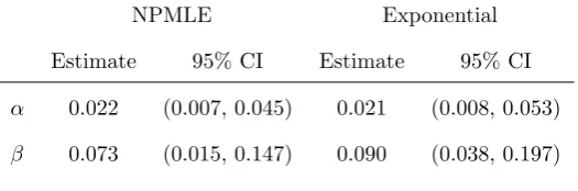
Table 2: Estimates and confidence intervals of false positive and false negative CAV diagnosis probabilities
for models based on a non-parametric failure time distribution and an exponential failure time distribution.
NPMLE Exponential
Estimate 95% CI Estimate 95% CI
α 0.022 (0.007, 0.045) 0.021 (0.008, 0.053)
[image:14.595.176.439.225.312.2]β 0.073 (0.015, 0.147) 0.090 (0.038, 0.197)
Table 2 gives the estimated diagnostic error rates using the NPMLE and also based on a parametric model
assuming a constant hazard of progression, implying exponentially distributed onset times. The estimated
error probabilities are broadly similar - in each case there is estimated to be a greater risk that the angiogram
will fail to detect the presence of CAV, than to over-diagnose it. The estimated false negative probability,
β, is slightly lower for the non-parametric model.
Figure 3 gives the NPMLE of the onset distribution compared to the exponential estimate from the
parametric model. There is some suggestion of an increasing hazard of onset since the non-parametric
estimate is somewhat lower than the parametric in the period 1 to 2 years post-transplantation.
7
Discussion
In addition to allowing the misclassification probabilities to depend on time, a relatively straightforward
extension would be to allow dependence on explanatory variables. A more challenging extension is to
incorporate the effect of explanatory variables into the failure time distributionF. One approach would be to adopt an accelerated failure time model where logTj =Z
0
jθ+j for a p-dimensional covariateZj with
corresponding p-dimensional regression coefficient θ, wherej are independent and identically distributed
residuals with unknown distribution ˜F. In the standard interval censored case, Rabinowitz et al (1995) considered estimation via a family of score statistics. This approach can be adapted for misclassified data.
LetXij,u= logXij−Z 0
0 1 2 3 4 5 6 0.0
0.1 0.2 0.3 0.4
Time (years)
[image:15.595.183.422.97.321.2]F^
Figure 3: NPMLE for probability of disease onset (solid line) and parametric exponential estimate (dashed
line) for CAV data.
the support regions of the NPMLE for ˜F given a particular value,u, of the regression coefficient. Estimation can be based upon a score statistic of the form
S(u) =
n
X
j=1 Zj
Pnj+1
i=1 {g(F(Xij,u))−g(F(Xij−1,u))}˜γij
Pnj+1
i=1 ({F(Xij,u)−F(Xij−1,u)}γ˜ij)
whereXi0,u=−∞andXini+1,u=∞andgis some function with domain [0,1] satisfyingg(0) =g(1) = 0, with this condition ensuring Eu(S(u)) =0. The efficiency of this estimator will depend on the choice ofg.
An adaptive procedure for choosingg, similar to that proposed by Rabinowitz et al (1995), may be possible, but is beyond the scope of this paper.
In applications of the model, the assumption of independence of the observations conditional on the
failure time is likely to be key. In principle, a more general form forγij(α, β) could be adopted allowing the
individual classifications to be correlated, for instance via a shared multivariate binary copula. However, it
is not clear how this would affect the support set ofF or the joint identifiability ofF andθ.
In the application on onset of CAV, an implicit assumption that censoring due to death was made. The
data used was restricted to the first 6 years of follow-up, where death from CAV is relatively rare. However,
would be to adopt an illness-death type model with misclassified illness status (Sharples et al, 2003; Teeple
and Brown, 2015). A fully non-parametric approach in this case would require the extension of the methods
of Frydman and Szarek (2009) for three-state illness-death Markov models.
References
Abrevaya J, Huang J (2005) On the bootstrap of the maximum score estimator. Econmetrica 73:1175–1204
Balasubramanian R, Lagakos S (2003) Estimation of a failure time distribution based on imperfect diagnostic
tests. Biometrika 90:171–182
Banerjee M, Wellner J (2001) Likelihood ratio tests for monotone functions. Annals of Statistics 29:1699–1731
Banerjee M, Wellner J (2005) Confidence intervals for current status data. Scandinavian Journal of Statistics
32:405–424
Barlow R, Bartholomew D, Bremner J, Brunk H (1972) Statistical Inference Under Order Restrictions. The
Theory and Application of Isotonic Regression. Wiley
Betensky R, Rabinowitz D, Tsiatis A (2001) Computationally simple accelerated failure time regression for
interval censored data. Biometrika 88:703–711
B¨ohning D (1985) Numerical estimation of a probability measure. Journal of Statistical Planning and
Infer-ence 11:57–69
B¨ohning D, Schlattmann P, Dietz E (1996) Interval censored data: A note on the nonparametric maximum
likelihood estimator of the distribution function. Biometrika 83:462–466
Espeland M, Platt O, Gallagher D (1989) Joint estimation of incidence and diagnostic error rates from
irregular longitudinal data. Journal of the American Statistical Association 84:972–979
Frydman H, Szarek M (2009) Nonparametric estimation in a Markov ’illness-death’ process from interval
censored observations with missing intermediate transition status. Biometrics 65:143–151
van de Geer S (2003) Asymtotic theory for maximum likelihood in nonparametric mixture models.
Compu-tational Statistics and Data Analysis 41:453–464
Groeneboom P, Wellner JA (1992) Information Bounds and Nonparametric Maximum Likelihood Estimation,
Gr¨uger J, Kay R, Schumacher M (1991) The validity of inferences based on incomplete observations in disease
state models. Biometrics 47:595–605
Jongbloed G (1998) The iterative convex minorant algorithm for nonparametric estimation. Journal of
Com-putational and Graphical Statistics 7(3):310–321
Laird N (1978) Nonparametric maximum likelihood estimation of a mixing distribution. Journal of the
American Statistical Association 73:805–811
Lawson C, Hanson R (1974) Solving Least Squares Problems. Englewood Cliffs: Prentice-Hall
Lesperance M, Kalbfleisch J (1992) An algorithm for computing the nonparametric mle of a mixing
distri-bution. Journal of the American Statistical Association 87:120–126
Lindsay BG (1983) The geometry of mixture likelihoods: A general theory. Annals of Statistics 11(1):86–94
Maathuis M, Hudgens M (2011) Nonparametric inference for competing risks current status data with
continuous, discrete or grouped observation times. Biometrika 98:325–340
McKeown K, Jewell N (2010) Misclassification of current status data. Lifetime Data Analysis 16:215–230
Murphy S, van der Vaart A (1997) Semiparametric likelihood ratio inference. Annals of Statistics 25:1471–
1509
Ng MP (2002) A modification of Peto’s nonparametric estimation of survival curves for interval-censored
data. Biometrics 58:439–442
Politis D, Romano J (1994) Large sample confidence regions based on subsamples under minimal assumptions.
Annals of Statistics 22:2031–2050
Rabinowitz D, Tsiatis A, Aragon J (1995) Regression with interval-censored data. Biometrika 82:501–513
Richardson B, Hughes J (2000) Product limit estimation for infectious disease data when the diagnostic test
for the outcome is measured with uncertainty. Biostatistics 1:341–354
Sal y Rosas V, Hughes J (2011) Nonparametric and semiparametric analysis of current status data subject
to outcome misclassification. Statistical Communications in Infectious Diseases 3(1):7
Sen B, Xu G (2015) Model based bootstrap mmethod for interval censored data. Computational Statistics
Sharples LD, Jackson CH, Parameshwar J, Wallwork J, Large SR (2003) Diagnostic accuracy of
coro-nary angiography and risk factors for postheart-transplant cardiac allograft vasculopathy. Transplantation
76(4):679–682
Tang R, Banerjee M, Kosorok M (2012) Likelihood based inference for current status data on a grid: A
boundary phenomenon and an adaptive inference procedure. Annals of Statistics 40:45–72
Teeple EA, Brown ER (2015) Adjusting for time-dependent sensitivity in an illness-death model, with
ap-plication to mother-to-child transmission of hiv. Statistics in Medicine 34:1277–1292
Turnbull B (1976) The empirical distribution function with arbitrarily grouped, censored and truncated
data. Journal of the Royal Statistical Society: Series B 38:290–295
Wang Y (2007) On fast computation of the non-parametric maximum likelihood estimate of a mixing
dis-tribution. Journal of the Royal Statistical Society: Series B 69:185–198
Wang Y (2010) Maximum likelihood computation for fitting semiparametric mixture models. Statistics and
Computing 20:75–86
Wellner J, Zhan Y (1997) A hybrid algorithm for computation of the nonparametric maximum likelihood
estimator from censored data. Journal of the American Statistical Association 92:945–959
Zhu L, Tong X, Sun J (2008) A transformation approach for the analysis of interval-censored failure time