http://www.scirp.org/journal/jmp ISSN Online: 2153-120X
ISSN Print: 2153-1196
DOI: 10.4236/jmp.2019.107053 Jun. 20, 2019 729 Journal of Modern Physics
The Solution Cosmological Constant Problem
Jaykov Foukzon1, Elena Men’kova2, Alexander Potapov3
1Department of Mathematics, Israel Institute of Technology, Haifa, Israel
2All-Russian Research Institute for Optical and Physical Measurement, Moscow, Russia
3Kotel’nikov Institute of Radioengineering and Electronics, Russian Academy of Sciences, Moscow, Russia
Abstract
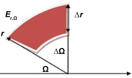
The cosmological constant problem arises because the magnitude of vacuum energy density predicted by the Quantum Field Theory is about 120 orders of magnitude larger then the value implied by cosmological observations of ac-celerating cosmic expansion. We pointed out that the fractal nature of the quantum space-time with negative Hausdorff-Colombeau dimensions can resolve this tension. The canonical Quantum Field Theory is widely believed
to break down at some fundamental high-energy cutoff Λ∗ and therefore
the quantum fluctuations in the vacuum can be treated classically seriously only up to this high-energy cutoff. In this paper we argue that the Quantum Field Theory in fractal space-time with negative Hausdorff-Colombeau di-mensions gives high-energy cutoff on natural way. We argue that there exists hidden physical mechanism which cancels divergences in canonical
4, 4
QED QCD , Higher-Derivative-Quantum gravity, etc. In fact we argue that
corresponding supermassive Pauli-Villars ghost fields really exist. It means that there exists the ghost-driven acceleration of the universe hidden in cosmological constant. In order to obtain the desired physical result we ap-ply the canonical Pauli-Villars regularization up to Λ∗. This would fit in the observed value of the dark energy needed to explain the accelerated ex-pansion of the universe if we choose highly symmetric masses distribution between standard matter and ghost matter below the scale Λ∗, i.e.,
( )
( )
. . , , eff, eff
s m g m
f µ −f µ µ=mc µ µ≤ µ c< Λ∗ The small value of the
cos-mological constant is explained by tiny violation of the symmetry between standard matter and ghost matter. Dark matter nature is also explained using a common origin of the dark energy and dark matter phenomena.
Keywords
Cosmological Constant Problem, Quantum Field Theory, Vacuum Energy Density, Quantum Space-Time, Hausdorff-Colombeau Dimension, Quantum How to cite this paper: Foukzon, J.,
Men’kova, E. and Potapov, A. (2019) The Solution Cosmological Constant Problem.
Journal of Modern Physics, 10, 729-794.
https://doi.org/10.4236/jmp.2019.107053
Received: February 5, 2019 Accepted: June 17, 2019 Published: June 20, 2019
Copyright © 2019 by author(s) and Scientific Research Publishing Inc. This work is licensed under the Creative Commons Attribution International License (CC BY 4.0).
http://creativecommons.org/licenses/by/4.0/
DOI: 10.4236/jmp.2019.107053 730 Journal of Modern Physics
Fluctuations, High-Energy Cutoff, Canonical Pauli-Villars Regularization, Universe
1. Introduction
1.1. The Formulation of the Cosmoloigical Constant Problem
The cosmological constant problem arises at the intersection between general relativity and quantum field theory, and is regarded as a fundamental unsolved problem in modern physics. A peculiar and truly quantum mechanical feature of the quantum fields is reminded that they exhibit zero-point fluctuations every-where in space, even in regions which are otherwise “empty” (i.e. devoid of mat-ter and radiation). This vacuum energy density is believed to act as a contribu-tion to the cosmological constant λ appearing in Einstein’s field equations from 1917,
4
1 8π
2
G
R g R T
c
µν − µν = µν′ (1)
where Rµν and R refer to the curvature of space-time, gµν is the metric, Tµν′
is the the energy-momentum tensor,
4
1 0 0 0
0 1 0 0
0 0 1 0
8π
0 0 0 1
c
T T
G
µν µν λ
−
′ = +
−
(2)
where Tµν is the energy-momentum tensor of matter. Thus T00′ =T00+ελ, Tαβ′ =Tαβ+δαβ λP , where
4 8π .
P c G
λ λ
ε = − = λ (3)
Reminding that under Lorentz transformations
(
ελ,Pλ)
→ελ′,(
ελ,Pλ)
→Pλ′ the quantities ελ and Pλ are changes by the law2 2
2 , 2 .
1 1
P P
P
λ λ λ λ
λ λ
ε β β ε
ε
β β
+ +
′ = ′=
− − (4)
Thus for the quantities ελ and Pλ Lorentz invariance holds by Equation (3)
[1].
In modern cosmology it is assumed that the observable universe was initially vacuumlike, i.e., the cosmological medium was non-singular and Lorentz inva-riant. In the earlier, non-singular Friedmann cosmology, the Friedmann un-iverse comes into being during the phase transition of an initial vacuumlike state to the state of “ordinary” matter [2][3].
Robert-DOI:10.4236/jmp.2019.107053 731 Journal of Modern Physics
son-Walker metric [2]. Robertson-Walker metric reads
( )
2(
)
2 2 2 2 2 2 2
2
d
d d d sin d .
1
r
s t a t r
kr θ θ ϕ
= − + +
−
(5)
For such a metric, the Ricci curvature scalar is R= −6k and it is said that
space has the curvature k. The scaling factor a t
( )
rescales this curvature for a given time t, producing a curvature k t( )
=k a t( )
. The scaling factor a t( )
isgiven by two independent Friedmann equations for modeling a homogeneous, isotropic universe reads
(
)
2 2
, 3
3 6
G G
a = εa −k a= − ε+ p (6)
and the equation of state
( )
,p= p ε (7)
where p is pressure and ε is a density of the cosmological medium. For the
case of the vacuumlike cosmological medium equation of state reads [2][3][4]:
.
p= −ε (8)
By virtue of Friedman’s Equation (6) in the Universe filled with a vacuum-like medium, the density of the medium is preserved, i.e. ε=const, but the scale
factor a t
( )
grows exponentially. By virtue of continuity, it can be assumed that the admixture of a substance does not change the nature of the growth of the latter, and the density of the medium hardly changes. This growth, interpreted by analogy with the Friedmann models as an expansion of the universe, but al-most without changing the density of the medium! was named inflation. The idea of inflation is the basis of inflation scenarios [2].Non-singular cosmology [2][4] suggests that the initial state of the observable universe was vacuum-like, but unstable with respect to the phase transition to the ordinary non-Lorentz-invariant medium. This, for example, takes place if, by virtue of the equations of state of the medium, a fluctuation decrease in its den-sity d violates the condition of vacuum-like degeneration, p= −ε or, which is
the same, 3p+ = −ε 2ε <0, replacing it with 2ε 3p ε 0.
− < + < (9)
According to Friedman’s equations, it corresponds to an accelerated expan-sion of the cosmological medium, accompanied by a drop in its density, which makes the process irreversible [2]. The impulse for expansion in this scenario, the vacuum-like environment, is not reported to itself (bloating), but to the emerging Friedmann environment.
con-DOI: 10.4236/jmp.2019.107053 732 Journal of Modern Physics
stant problem. As well known zeropoint energy density of scalar quantum field, etc. is divergent
( )
(
)
2 2 2 2
vac 3 0
2π
d .
2π
c
m p m c p p
ε =
∫
∞ + = ∞ (10)
In order to avoid difficulties mentioned above, in article [1] Zel’dovich has applied canonical Pauli-Villars regularization [7][8] and formally has obtained a finite result (his formulas [1], Eqs. (VIII.12)-(VIII.13) p. 228)
( ) (
4)
4vac vac 0
1
ln d ,
8 8π
c
p f
G λ
ε = − =
∫
∞ µ µ µ µ= (11)where
( )
( )
2( )
40 f µ µd 0 f µ µ µd 0 f µ µ µd 0.
∞ ∞ ∞
= = =
∫
∫
∫
(12)Remark 1.1.1. Unfortunately, Equation (11) and Equation (12) give nothing in order to obtain desired numerical values of the zero-point energy density ε.
In his paper [1], Zel’dovich arrives at a zero-point energy (his formula (IX.1))
3
17 3 10 2
vac ~ 10 g cm , ~ 10 cm ,
mc m
ε = λ − −
(13)
where m (the ultra-violet cut-of) is taken equal to the proton mass. Zel’dovich notes that since this estimate exceeds observational bounds by 46 orders of mag-nitude it is clear that “... such an estimate has nothing in common with reality”.
In his paper [1], Zel’dovich wrote: Recently A. D. Sakharov proposed a theory of gravitation, or, more precisely, a justification GR equation based on consider-ation of vacuum fluctuconsider-ations. In this theory, the essential assumption is that there is some elementary length L or the corresponding limiting momentum
0
p = L. Shorter lengths or for large impulses theory is not applicable.
Sakha-rov gets the expression of gravitational constant G through L or p0 (his
for-mula (IX.6))
3 2 3 2 0
.
c L c
G
p
= =
(14)
This expression has been known since the days of Planck, but it was read “from right to left”: gravity determines the length L and the momentum p0.
According to Sakharov, L and p0 are primary. Substitute (IX. 6) in the
expres-sion (IX. 4), we get
6 5 6 7
vac 2 3 vac 2 3
0 0
, .
m c m c
p p
ρ = ε =
(15)
That is expressions that the first members (in the formulas (VIII.10), (VIII. 11)) which are vanishes (with p0→ ∞). Thus, we can suggest the following
DOI:10.4236/jmp.2019.107053 733 Journal of Modern Physics
which the theory is non applicable; along with other implications, modifying the theory gives different from zero vacuum energy; general considerations make it likely that the effect is portional 2
0
p− . Clarification of the question of the
exis-tence and magnitude of the cosmological constant will also be of fundamental importance for the theory of elementary particles.
Nonclassical Assumptions
(I) In contrast with Zel’dovich paper [1] we assume that Poincaré group is deformed at some fundamental high-energy cutoff Λ∗ [9] [10][11] in accor-dance with the basis of the following deformed Poisson brackets
{
}
(
) {
}
{
}
1 0 0
1 0
, , , 0,
,
x x x x p p
x p p
µ ν µ ν ν µ µ ν
µ ν µν µ ν
η η
η η
−
−
= − =
= − +
(16)
where µ ν, =0,1, 2, 3, η = + − − −µν
(
1, 1, 1, 1)
and is a parameter identified as the ratio between the high-energy cutoff Λ∗ and the light speed. The correspond-ing to (16) momentum transformation reads [11](
)
( ) (
)
(
)
( ) (
)
( ) (
)
( ) (
)
2 0 0
0 1 1
0 0
1 1
0 0
, ,
1 1 1 1
, ,
1 1 1 1
x x
x
x x
y z
y z
x x
p up c p up
p p
c p up c p up
p p
p p
c p up c p up
γ γ
γ γ γ γ
γ γ γ γ
− −
− −
− −
′= ′=
+ − − + − −
′ = ′=
+ − − + − −
(17)
and coordinate transformation reads [11]
(
)
( ) (
)
( ) (
(
)
)
( ) (
)
( ) (
)
2
1 1
0 0
1 1
0 0
, ,
1 1 1 1
, ,
1 1 1 1
x x
x x
t ux c x ut
t x
c p up c p up
y z
y z
c p up c p up
γ γ
γ γ γ γ
γ γ γ γ
− −
− −
− −
′= ′=
+ − − + − −
′= ′=
+ − − + − −
(18)
where 2 2
1 u c
γ = − . It is easy to check that the energy E=c, identified as
the high-energy cutoff Λ∗, is an invariant as it is also the case for the funda-mental length lΛ∗ =c E= .
Remark 1.1.2. Note that the transformation (17) defined in p-space and the transformation (1.1.18) defined in x-space becomes Lorentz for small energies
and momenta and defines a large invariant energy 1
lΛ−∗. The high-energy cutoff
∗
Λ is preserved by the modified action of the Lorentz group [9][10].
This meant that the canonical concept of metric as quadratic invariant col-lapses at high energies, being replaced by the non-quadratic invariant [9]:
(
)
2
0
, 1
ab a b p p p
l p
η
Λ∗
=
+ (19)
or by the non-quadratic invariant
(
)
2
0
, 1
ab a b p p p
l p
η
Λ∗
=
− (20)
where 1
, , 0,1, 2, 3
DOI: 10.4236/jmp.2019.107053 734 Journal of Modern Physics
Remark 1.1.3. Note that:
1) the invariant (16) is infinite for the new negative invariant energy scale of
the theory 1
l−∗
∗ Λ
Λ = − , and it’s not quadratic for energies close or above and 2) the invariant (17) is infinite for the new positive invariant energy scale of
the theory 1
l ∗
−
∗ Λ
Λ = .
Remark 1.1.4. It is also clear from Equation (16) and Equation (17) that the symmetry of positive and negative values of the energy is broken. The two theo-ries with the two signs of lΛ obviously are physically distinct; and we know of no theoretical argument which fixes the signs of Λ
The massive particles have a positive invariant 2
0
p > which can be
identi-fied with the square of the mass 2 2
p =m , (c=1). Thus in the case of the
in-variant (16) we obtain
(
)
(
)
2 2
2 1
0
0 2
0
, ,
1
p p
m p l
l ∗p ∗
− Λ Λ
− = ∈ − ∞
+ (21)
From Equation (18) we obtain
(
)
2 4 2
2 2
0 2 2 2 2 2 2
1
.
1 1 1
m l m l
p p m
m l m l m l
∗ ∗
∗ ∗ ∗
Λ Λ
Λ Λ Λ
= + + +
− − − (22)
In the case of the invariant (17) we obtain
(
)
(
)
2 2
2 1
0
0 2
0
, , .
1
p p
m p l
l ∗p ∗
− Λ Λ
− = ∈ −∞
− (23)
From Equation (20) we obtain
(
)
2 4 2
2 2
0 2 2 2 2 2 2
1
.
1 1 1
m l m l
p p m
m l m l m l
∗ ∗
∗ ∗ ∗
Λ Λ
Λ Λ Λ
= − − + +
− − − (24)
The action for a scalar field ϕ must be invariant under the deformed Lo-rentz transformations. The invariant action reads [10]
(
)(
)
24 2
0
1
d .
2 1 2
ab
a b m
S x
l
η ϕ ϕ
ϕ ϕ
∗
Λ
∂ ∂
= +
+ ∂
∫
(25)Thus there is no linear field equation.
Remark 1.1.5.Throughout this paper, we use below high-energy cutoff Λ∗
the perturbative expansion
(
)(
)
2( )
4 2
1
d .
2 2
ab
a b m
S x η ϕ ϕ ϕ O lΛ∗
= ∂ ∂ + +
∫
(26)and dealing in Lorentz invariant approximation
(
)(
)
24 2
1
d .
2 2
ab
a b m S xη ∂ ϕ ∂ ϕ + ϕ
∫
(27)
DOI:10.4236/jmp.2019.107053 735 Journal of Modern Physics
(II) The canonical concept of Minkowski space-time collapses at a small
dis-tance 1
lΛ∗ = Λ∗− to fractal space-time with Hausdorff-Colombeau negative
di-mension and therefore the canonical Lebesgue measure 4
d x being replaced by
the Colombeau-Stieltjes measure with negative Hausdorff-Colombeau dimen-sion D−:
( )
(
)
(
(
( )
)
4)
d x, ε vε s x d x ,
ε
η ε = (28)
where
(
(
( )
)
)
( )
1 D
vε s x s x
ε
ε
ε
− −
= +
and s x
( )
x xµ µ
= , see Section 3 and
[12].
(III) The canonical concept of momentum space collapses at fundamental
high-energy cutoff Λ∗ to fractal momentum space with Hausdorff-Colombeau
negative dimension and therefore the canonical Lebesgue measure 3
dk, where
(
k k kx, y, z)
=
k being replaced by the Hausdorff-Colombeau measure
( )
( ) ( )
1, d d
d ,
D D
D D
D D
D D D p p
p
ε ε
ε ε
+ +
+ −
− −
− + − −
∆ ∆ ∆
=
+ +
k
k k
(29)
where
( )
2π 2(
)
2
D
D± ± D±
∆ = Γ and p= k = kx+ky+kz and where
6
D+− D− ≤ − , see Section 3 and ref. [9]. Hausdorff-Colombeau measure (29)
avoids classical divergence (10) of the zeropoint energy εvac
( )
m and insteadEquation (10) one obtains
(
)
3 2 2( ) ( )
2 2 2 4vac , 0 d d .
p
p D
p m
p m p p m D D pp p
p
ε
ε
ε ∗
− ∗
∞
+ −
∗ ∗
+
= + + ∆ ∆
+
∫
∫
(30)See Section 5 and ref. [12].
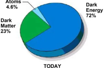
Remark 1.1.6. If we take the Planck scale (i.e. the Planck mass) as a cut-off, the vacuum energy density εvac
(
p m∗,)
is 10121 times larger than the observed dark energy density εde. Several possible approaches to the problem of vacuumenergy have been discussed in the contemporary literature, for the review see [5],
[12]. They can be roughly devided into five different groups: 1) Modification of gravity on large scales. 2) Anthropic principle.
3) Symmetry leading to εvac =0. 4) Adjustment mechanism, see. 5) Hidden
nonstandard dark matter sector and corresponding hidden symmetry leading to
vac 0
ε , see [12].
(IV) We assume that there exists the nonstandard dark matter sector formed by ghost particles, see [12].
1.2. Zel’dovich Approach by Using Pauli-Villars Regularization Revisited. Ghosts as Physical Dark Matter
DOI: 10.4236/jmp.2019.107053 736 Journal of Modern Physics
( )
(
)
3 0 2 2 2 0 2 2 2( )
1
4π d d ,
2 2π
c
p p p K p p p KI
ε µ =
∫
∞ +µ =∫
∞ +µ = µ (31)
where µ=m c0 . From Equation (31) one obtains [1]
( )
4( )
0 2 2
d
. 3
K p p
p KF
p
µ µ
µ
∞
= =
+
∫
(32)For fermionic quantum field one obtains
( )
KI( ) ( )
,p 4KF( )
.ε µ = µ µ = − µ (33)
Thus free vacuum energy density ε and corresponding pressure p is
( )
,( )
.i i i i
i i
C I P C F
ε =
∑
µ =∑
µ (34)From Equation (34) by using Pauli-Willars regularization [7] [8] in general case one obtains [1]
( ) ( )
d ,( ) ( )
d .f I P f F
ε=
∫
µ µ µ =∫
µ µ µ (35)In order to obtain asymptotical expansion on the parameter p0 of the
quan-tity
(
)
0 3 2 2vac 0, 0 d
p
p m p p m
ε =
∫
+ let us evaluate now the following integral(
)
0 00
2 2 2 2 2 2 2 2 2
0
0 0
2 2
2 2 2 3 3
2 2
0
, d d d
d 1 d 1 d
p
p p
p
p p p
p p
I p p p p p p p p p p
p p p p p p p
p p
µ
µ
µ µ
µ µ
µ µ µ µ
µ µ
µ
= + = + + +
= + = + + +
∫
∫
∫
∫
∫
∫
(36)
and
(
)
0 00
4 4 4
0
2 2 2 2 2 2
0 0
4 3
2 2 2
0
2
1 d 1 d 1 d
,
3 3 3
1 d 1 d
,
3 3
1
p
p p
p
p p
p
p p p p p p
F p
p p p
p p p p
p
p µ
µ µ
µ µ
µ µ µ
µ µ
= = +
+ + +
= +
+ +
∫
∫
∫
∫
∫
(37)where pµ =rµ,r>1,µ p<1r<1. Note that
2 2 4 6
2 2 4 6
2 4 6
2 2 2 3 3 2
2 3
1 1 1
1 1
2 8 16
1 1 1
1
2 8 16
p p p p
p p p p p
p
p p
µ µ µ µ
µ µ µ
µ µ
+ = + − + +
+ = + = + − + +
(38)
By inserting Equation (38) into Equations (36) one obtains
(
)
4 4 2 2 4 0 6 5( )
80 1 0 0 2 0
0
1 1 1 1
, ln ,
4 4 8 32
p
I p C p p p O
p µ
µ µ µ µ µ
µ
−
= + + − − +
(39)
where 4 2 2 2
1 0 d
p
DOI:10.4236/jmp.2019.107053 737 Journal of Modern Physics 1
2 2 4 6
2 2 4 6
1 3 5
1 1
2 8 16
p p p p
µ − µ µ µ
+ = − + − +
(40)
By inserting Equation (40) into Equation (37) one obtains
(
)
4 4 2 2 4 0 6 5( )
80 2 0 0 2 0
0
1 1 1 5
, ln .
12 12 8 32
p
F p C p p p O
p µ
µ µ µ µ µ
µ
−
= + − + + +
(41)
By inserting Equation (39) and Equation (41) into Equations (35) one obtains
( )
( )
( )
( ) (
)
( )
( )
( )
( )
( )
eff eff eff
eff eff eff
eff eff eff
4 2 2 4
0 0 1 0
0 0 0
4 6 8 5
0 2
0 0 0 0
4 2 2 4
0 0 2 0
0 0 0
1 1 1
d d ln d
4 4 8
1 1 1
ln d d ,
8 32
1 1 1
d ln d
12 12 8
1 8
p f p f C p f
f f O f p
p
p p f p f d C p f
µ µ µ
µ µ µ
µ µ µ
ε µ µ µ µ µ µ µ µ
µ µ µ µ µ µ µ µ µ
µ µ µ µ µ µ µ µ
− = + + − + − + = − + + −
∫
∫
∫
∫
∫
∫
∫
∫
∫
( ) (
)
( )
( )
eff eff eff
4 6 8 5
0 2
0 0 0 0
5 1
ln d d .
32
f f O f p
p
µ µ µ
µ µ µ µ+ µ µ µ+ µ µ −
∫
∫
∫
(42)
We choose now
( )
( )
( )
eff eff eff
2 4
0 0 0
d d d 0.
f f f
µ µ µ
µ µ= µ µ µ= µ µ µ=
∫
∫
∫
(43)By inserting Equation (43) into Equations (42) one obtains
(
)
( ) (
)
( )
(
)
( ) (
)
( )
eff eff 4 2 eff 0 0 4 2 eff 0 0 1ln d ,
8 1
ln d .
8
f O p
p f O p
µ
µ
ε µ µ µ µ µ
µ µ µ µ µ
− − = + = − +
∫
∫
(44)Taking the limit p→ ∞ in Equation (44) gives
(
)
( ) (
)
(
)
( ) (
)
eff eff 4 eff 0 4 eff 0 1ln d , 8
1
ln d . 8
f
p f
µ
µ
ε µ µ µ µ µ
µ µ µ µ µ
=
= −
∫
∫
(45)
Thus finally we obtain [3]
(
)
(
)
eff( ) (
)
44 eff eff
0
1
ln d .
8 8π
c
p f
G
µ
ε µ = − µ =
∫
µ µ µ µ= Λ (46)Remark 1.2.1. Remind that Pauli-Villars regularization consists of introduc-ing a fictitious mass term. For example, we would replace a propagator
(
2 2)
0
1 k −m +i , by the regulated propagator
( )
22 2 2 2 2 2
0 0
0
1
,
N i N i
i i
i i
a a
k
k m i k m i k m i
= =
∆ = = −
− + − + − +
∑
∑
(47)where a0=1 and m ii, =1, 2,,N can be thought of as the mass of a fictitious
heavy particle, whose contribution is subtracted from that of an ordinary particle.
Assume that 2 2
1
i
se-DOI: 10.4236/jmp.2019.107053 738 Journal of Modern Physics
ries in 2
k +i we get
( )
(
)
(
)
2 2
2 2 3
0 0 0
2 2
1 .
N i N i i N
i i i
a a m
k O
k i k i k i
= = =
∆ = + +
+ + +
∑
∑
∑
(48)
For a renormalizable theory the maximum supercriticial power of divergence of any integral is quadratic, so that the
( )
61
O k terms are ultraviolet finite.
The finiteness of the regulated integral is then guaranteed by requiring that
2
0 0, 0 0.
N N
i i i
i= a = i= a m =
∑
∑
(49)Remark 1.2.2. Note that in order to apply Pauli-Villars regularization to QFT with Lagrangian L
(
ϕ ψ, ,∂µϕ ψ,∂µ)
we would replace the Lagrangian(
ϕ ψ, ,∂µϕ ψ,∂µ)
L by Lagrangian L
(
ϕ ψ, ,∂µϕ ψ,∂µ)
, where [7]:( )
( )
(
2)
( )
( )
(
2)
, , , ,
n n n n n n
n n
x x b x x x c x
ϕ =ϕ +
∑
ϕ µ ψ =ψ +∑
ψ (50)where commutator for ϕn and anticommutator for ψn reads
(
) (
)
(
)
(
) (
)
{
}
(
)
2 2 2
2 2 2
, , , , ,
, , , , .
m m n n n n mn
m m n n n n mn
x x i x x
x x i S x x
ϕ µ ϕ µ ρ µ δ
ψ ψ ε δ
′ = − ∆ − ′
′ = − − ′
From Equations (50)-Equations (51) one obtains
( ) ( )
(
)
( ) ( )
(
)
2 2
0
2 0
, , ,
, , .
N
n n n
n N
n n n n
n
x x i b x x
x x i c c S x x
ϕ ϕ ρ µ
ψ ψ ε
=
=
′ = ∆ − ′
′ = − − ′
∑
∑
(52)Assume now that
2 2 2 2
0 0, 0 0, 0 0, 0 0.
N N N N
n n n n n n n n n n n n
n= ρ b = n= ρ µb = n= ε c c = n= ε c c =
∑
∑
∑
∑
(53)From Equations (53) it follows directly that QFT with Lagrangian
(
ϕ ψ, ,∂µϕ ψ,∂µ)
L is finite QFT with indefinite metric [4], see Remark 1.2.1.
Remark 1.2.3. Note that “bad ghosts” represent general meaning of the word “ghost” in theoretical physics: states of negative norm [7] or fields with the wrong sign of the kinetic term, such as Pauli--Villars ghosts ϕ, whose existence allows the probabilities to be negative thus violating unitarity. The quadratic
la-grangian 2
ϕ
L for ϕ begins with a wrong sign kinetic term [in (+ − − −) sig-nature]
2 1
2 µ
ϕ= − ∂ ∂ϕ ϕµ +
L (54)
Remark 1.2.4. Note that in order to obtain Equations (44), the standard quantum fields do not need to couple directly to the ghost sector. In this paper the ghost sector is considered as physical mechanism which acts only on a func-tion f
( )
µ in Equations (43). It means that there exists the ghost-driven acce-leration of the universe hidden in cosmological constant Λ.DOI:10.4236/jmp.2019.107053 739 Journal of Modern Physics
gives rise to a fascinating modification of gravity in the IR. However, no modifi-cations of gravity can be seen directly, and no cosmological experiment can dis-tinguish the ghost-driven acceleration from a cosmological constant.
Remark 1.2.6. In order to obtain desired physical result from Equations (45), i.e.,
29 3 47 4 3 5
vac 0.7 10 g cm 2.8 10 GeV c
ε = × − ⋅ − = × − (55)
we assume that
( )
s m. .( )
g m. .( )
,f µ = f µ + f µ (56)
where fs m. .
( )
µ corresponds to standard matter and where fg m. .( )
µcorres-ponds to a physical ghost matter. Remark 1.2.7. We assume now that
( )
( )
effeff
, 1
0
n
O n
f µ µ µ µ
µ µ
−
> ≤
=
>
(57)
From Equation (57) and Equation (45) it follows directly that
(
)
(
)
eff( ) (
)
(
)
4 5
eff eff eff eff
0
1
ln d ln .
8
n
p f O
µ
µ = ε µ = µ µ µ µ ≤ µ− + µ
∫
(58)Remark 1.2.8. However serious problem arises from non-renormalizability of canonical quantum gravity with Einstein-Hilbert action
4
1
d .
16π
EH
S x g R
G
=
∫
− (59)For example taking Λ3 particles of energy a per unit volume gives the
gravi-tational self-energy density of order Λ6, i.e., the density ε
Λ diverges as Λ6
6
,
G
εΛ Λ (60)
where Λ is a high-energy cutoff [5].
In order to avoid these difficulties we apply instead Einstein-Hilbert action (59) the gravitational action which includes terms quadratic in the curvature tensor
(
)
4 2 2
d x g αR Rµν µν βR 2κ−R ,
ℑ = −
∫
− − + (61)Remark 1.2.9. Gravitational actions (61) which include terms quadratic in the curvature tensor are renormalizable [14]. The requirement that the graviton propagator behaves like p−4 for large momenta makes it necessary to choose
the indefinite-metric vector space over the negative-energy states. These nega-tive-norm states cannot be excluded from the physical sector of the vector space without destroying the unitarity of the S matrix, however, for their unphysical
behavior may be restricted to arbitrarily large energy scales Λ∗ by an appropri-ate limitation on the renormalized masses m2 and m0.
Remark 1.2.10. We assume that m c0 µeff,m c2 µeff.
Remark 1.2.11. The canonical Quantum Field Theory is widely believed to
DOI: 10.4236/jmp.2019.107053 740 Journal of Modern Physics
quantum fluctuations in the vacuum can be treated classically seriously only up to this high-energy cutoff, see for example [15]. In this paper we argue that Quantum Field Theory in fractal space-time with negative Hausdorff-Colombeau dimensions [12] gives high-energy cutoff on natural way.
2. Ghosts as Physical Dark Matter
2.1. Paulu-Villars Ghosts As Physical Dark Matter
Before explaining the role of PV ghosts, etc. as physical dark matter remind the idea of PV regularization as a conventional UV regularization. We consider, as an example, the scalar field theory with the interaction λϕ4. Lagrangian density
of this theory reads
2
2 4
0
1
.
2 2
m
µ µ
ϕ ϕ ϕ λϕ
= ∂ ∂ − +
L (62)
This theory requires UV regularization (e.g. in (2+1) and (3+1) dimensions). Let us show that it is sufficient to introduce N extra fields with large mass play-ing the role of the regularization parameter. Lagrangian density can be rewritten as follows
( )
2 2 40
0 0 0
1
1 : :,
2 2
, .
i
N i
i i
N N
i i i
i i
m
a
µ µ
ϕ ϕ ϕ λ ϕ
ϕ ϕ ϕ ϕ ϕ ϕ
=
= =
= − ∂ ∂ − +
= + = =
∑
∑
∑
L
(63)
Here the symbol “::” means that in perturbation theory we drop Feynman di-agrams with loops containing only one vertex. The ϕ0 is usual field with mass
0
m and the ϕi,i=1,,N is the extra field with mass m ii, =1,,N. It can be
shown that in (3+1)-dimensional theory the introduction of one PV field is suf-ficient for the ultraviolet regularization of perturbation theory in λ. One can show that momentum space Feynman diagrams in the original theory with La-grangian density (62) diverge no more than quadratically [16][17][18] (beside of vacuum diagrams) shown in Figure 1.
If we consider now Feynman diagrams in the theory with Lagrangian density (63) we see that propagators of fields ϕ0 and ϕ sum up in corresponding
di-agrams so that we obtain the following expression which plays the role of regu-larized propagator
( )
22 2 2 2 2 2
0 0
0
1
,
0 0 0
N j N j
j j
j j
a a
k
k m i k m i k m i
= =
∆ = = −
− + − + − +
∑
∑
(64)where 2 2 2 2 2
0 1 2 3
k =k −k +k +k . Integral corresponding to vacuum diagram is
( )
( )
( )
4 4
2
4 4 0 2 2
d d
. 0
2π 2π
N j
j
j a
k k
k
k m i
=
ℑ = ∆ =
− +
∑
∫
∫
(65)DOI:10.4236/jmp.2019.107053 741 Journal of Modern Physics Figure 1. One-loop massive
va-cuum diagram.
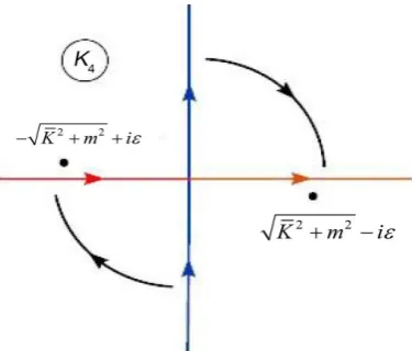
Remark 2.1.1. All the integrals in quantum field theory are written in Min-kowski space, however, the ultraviolet divergence appears for large values of modulus of momentum and it is useful to regularise it in Euclidean space [17]. Transition to Euclidean space can be achieved by replacing thr zeroth compo-nent of momentum k0 →ik4, where the integration over the fourth component
of momenta goes along the imaginary axis. To go to the integration along the real axis, one has to perform the (Wick) rotation of the integration contour by 90˚ (see Figure 2). This is possible since the integral over the big circle vanishes and during the transformation of the contour it does not cross the poles.
Then we get
3
2 0 d 0 2 2.
8π
N j E
E E j
E j a k i
k
k m
∞
=
ℑ =
+
∑
∫
(66)To do this integral, since it is convergent, we can deal with regularized integral
(
,)
8π2 d 0 2 3 2,N j E E j
E j a k i
k
k m
ε
ε Λ =
ℑ Λ =
+
∑
∫
(67)where ε0,Λ ∞ , i.e. ℑ
(
ε,Λ ≈ ℑ)
E. We assume now that Pauli-Villarscon-ditions given by Equations (48) holds. Let us consider now the quantity
(
,)
8π2 d 0 2 3 2,N j E E j
E j
a k i
k
k m
η η ε ε η
Λ
=
ℑ ℑ Λ =
+
∑
∫
(68)
where η∈
(
0,1]
, and therefore from Equation (68) we obtain2 0 2 0
0 8π d 8π d 0,
N N
E j j E j j E E
i i
k a k a k k
ηη ε ε
Λ Λ
= =
=
ℑ =
∫
∑
=∑
∫
≡ (69)since Equations (48) holds. From Equation (68) by differentiation we obtain
(
)
2 3
2 0 2 2 2
d
d ,
d 8π
N j j E
E j
E j
a m k i
k
k m
η ε
η η
Λ
=
ℑ =
+
∑
∫
(70)DOI: 10.4236/jmp.2019.107053 742 Journal of Modern Physics Figure 2. The Wick rotation of the integration contour.
(
)
2 3
2 0 2 2 2
0
0
2 1
2 0
d
d
d 8π
d 0, 8π
N j j E
E j
E j
N
j j E E
j
a m k i
k
k m
i
a m k k
η ε
η
η
ε
η η
Λ
= =
= Λ −
=
ℑ =
+
= ≡
∑
∫
∑
∫
(71)
since Equations (48) holds. From Equation (70) by differentiation we obtain
( )
(
)
( )
(
)
4 3 2
2 0 2 0 2 2 3
4 3
2 3
2 2
d
d ,
d 4π
d .
4π
N N j j E
j E
j j
E j
j j E
j E
E j
a m k i
k
k m
ia m k
k
k m
η ε
ε
η
η η
η
η
Λ
= =
Λ
ℑ = ℜ =
+
ℜ =
+
∑
∫
∑
∫
(72)
Note that
( )
(
)
4 3 4 2
2 0 d 2 2 3 2 2 2 .
4π 4π 4 16π
j j E j j j j
j E
j
E j
ia m k ia m i a m
k
m
k m
η
η η
η
∞ −
ℜ = =
+
∫
(73)
Thus
( )
21
2
0 0 0
d
d ln
d 16π
N N j j
j
j j
a m
η η η η
ηℑ =
∑
=∫
ℜ =∑
= (74)and
(
)
2
2
016π ln ,
N j j j
a m
η = η η η
ℑ =
∑
− (75)Therefore
(
,)
1 016π22 0,N j j j
a m
η η
ε =
=
ℑ Λ = ℑ = −
∑
≡ (76)since Equations (48) holds. Thus integral (65) corresponding to vacuum diagram by using Pauli-Villars renormalization identically equal zero, i.e.
( )
( )
( )
( )
4 4
2
4 4 0 2 2
d d
Ren 0.
0
2π 2π
N j
PV j
j a
k k
k
k m i
=
ℑ = ∆ = ≡
− +
DOI:10.4236/jmp.2019.107053 743 Journal of Modern Physics
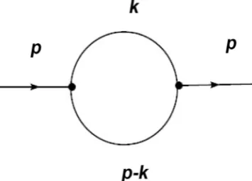
Let us consider now how this method works in the case of the simplest scalar diagram shown in Figure 3. The corresponding Feinman integral has the form
( )
( )
(
) (
)
4 2
4 2 2 2 2 2
0 0
1 d
.
2π 0 0
k p
k m i p k m i
ℑ =
− + − − +
∫
(78)Regularized Feinman integral (78) reads
( )
( )
(
) (
4)
2
4 0 2 2 2 2 2
d 1
,
2π 0 0
N j
reg j
j j
a k
p
k m i p k m i
=
ℑ =
− + − − +
∑
∫
(79)where N =1. To do this integral, since it is convergent, we can Wick rotate.
Then we get
( )
2( )
(
) (
4)
4 0 2 2 2 2 2
d
. 2π
N j
reg j
j j
a k
i p
k m p k m
=
ℑ =
+ − +
∑
∫
(80)The integral (80) can be written as
( )
( )
(
)
(
)
4 1
2
4 0 2
2 2 2
0
3 1
2 0 2 2 2 2
0
d d
2π 1
d
d .
8π 1
N j
reg j
j
N j E E
j
E j
a k
i
p x
k p x x m
a k k i
x
k p x x m
=
=
ℑ =
+ − +
=
+ − +
∑
∫ ∫
∑
∫ ∫
(81)
To do this integral, since it is convergent, we can deal with regularized integral
(
)
(
)
3 1
2
2 0 2 2 2 2
0
d
, , d .
8π 1
N j E E
reg j
E j
a k k i
p x
k p x x m
ε
ε Λ =
ℑ Λ =
+ − +
∑
∫ ∫
(82)Let us consider now the quantity
(
)
(
)
3 1
2
2 0 2 2 2 2
0
d
, , d .
8π 1
N j E E
j
E j
a k k i
p x
k p x x m
η ε ε
η
Λ =
ℑ Λ =
+ − +
∑
∫ ∫
(83)where η∈
(
0,1]
, and therefore from Equation (83) we obtain ℑ0(
p2, ,ε Λ ≡)
0, [image:15.595.284.462.574.702.2]since Equations (48) holds. From Equation (83) by differentiation we obtain
DOI: 10.4236/jmp.2019.107053 744 Journal of Modern Physics
(
)
(
)
(
)
(
)
(
)
(
)
2 3 1 22 0 2 2 2 3
0 2 2 2 0 3 1 2 3
2 2 2
0 1 2 2 0 d d
, , d
d 4π 1
, , , , 4π
d , , , d
1
1 d
.
4 1
N j j E E
j
E j
N
j j j
j
E E
j
E j
j
a m k k i
p x
k p x x m
i
a m p
k k
p x
k p x x m
x
p x x m
η ε ε
η η η ε η ε η η Λ = =
ℑ Λ = −
+ − +
− ℜ Λ
ℜ Λ + − + = − +
∑
∫ ∫
∑
∫ ∫
∫
(84)From Equation (84) we obtain
(
)
(
)
(
)
2 2 2
2 0
1
2 0 2 2
0 d , , , , , d 4π d . 16π 1 N
j j j j N j j j i
p a m p
i x
a
m p x x
η ε η ε
η
η
=
− =
ℑ Λ − ℜ Λ
= − − +
∑
∑
∫
(85)From Equation (85) we obtain
( )
1 1(
)
2
2 0 2 2
0 0
d
d .
16π 1
N
reg j j
j i
p a x
m p x x
η η
− =
ℑ = −
− +
∑
∫ ∫
(86)Note that
(
)
(
)
(
)
(
)
(
)
(
)
(
)
1 1
2 2 2 2
2 2 0
0
2 2 2 2
2 2 2 2
d
1 ln 1 1
1
1 1 ln 1 1
1 ln 1 1.
j j
j
j j
j j
m p x x m p x x
m p x x
m p x x m p x x
m p x x m p x x
η η η
η − − − − − − − = − + − + − − + = − + − + − − − −
∫
(87) Thus( )
(
)
(
)
(
)
{
(
)
(
)
}
(
)
(
)
{
1 1 1 22 0 2 2
0 0 1
1 2 2 2 2
2 0
0
1
2 2 2 2
2 0
1
1 2 2 2 2
2 0
0
d d
16π 1
d 1 1 ln 1 1
16π
1 ln 1
16π
d 1 1 ln 1 1
16π
N
reg j j
j
N
j j j
j
N
j j j j
N
j j j
j i
p a x
m p x x
i
a x m p x x m p x x
i
m p x x m p x x a
i
a x m p x x m p x x
η η = − = = − − = = − − = = − − =
ℑ = −
− + = − − + − + − − − + = − − + − +
∑
∫ ∫
∑
∫
∑
∑
∫
(
)
(
)
}
2 2 2 2
1 ln 1
j j
m p x− x m p x− x
− − −
(
)
(
)
{
(
)
(
)
}
(
)
(
)
{
(
)
(
)
}
12 2 2 2
0 0
2 0
2 2 2 2
0 0
1
2 2 2 2
1 1
2 0
2 2 2 2
1 1
d 1 1 ln 1 1
16π
1 ln 1
d 1 1 ln 1 1
16π
1 ln 1 .
i
x m p x x m p x x
m p x x m p x x
i
x m p x x m p x x
m p x x m p x x
− − − − − − − − = − − + − + − − − + − + − + − − −
∫
∫
(88)DOI:10.4236/jmp.2019.107053 745 Journal of Modern Physics
( )
{
(
)
(
)
(
)
(
)
}
(
)
(
)
{
(
)
(
)
}
1
2 2 2 2 2
0 0
2 0
2 2 2 2
0 0
1
2 2 2 2
1 1
2 0
2 2 2 2
1 1
d 1 1 ln 1 1
16π
1 ln 1
d 1 1 ln 1 1
16π
1 ln 1 .
reg
i
p x m p x x m p x x
m p x x m p x x
i
x m p x x m p x x
m p x x m p x x
− −
− −
− −
− −
ℑ = − − + − +
− − −
+ − + − +
− − −
∫
∫
(89)
We assume now that 2 2
1 1
m p− and from Equation (89) finally we obtain
( )
{
(
)
(
)
(
)
(
)
}
(
)
1
2 2 2 2 2
0 0
2 0
2 2 2 2 2 2
0 0 1
d 1 1 ln 1 1
16π
1 ln 1 .
reg
i
p x m p x x m p x x
m p x x m p x x O m p
− −
− − −
ℑ = − − + − +
− − − +
∫
(90)
Remark 2.1.2. The simple renormalizable models with finite masses
, 1, ,
i
m i= N which we have considered in the section many years regarded
only as constructs for a study of the ultraviolet problem of QFT. The difficulties with unitarity appear to preclude their direct acceptability as canonical physical theories in locally Minkowski space-time. However, for their unphysical beha-vior may be restricted to arbitrarily large energy scales Λ∗ mentioned above by an appropriate limitation on the finite masses mi.
2.2. Renormalizability of Higher Derivative Quantum Gravity
Gravitational actions which include terms quadratic in the curvature tensor are renormalizable. The necessary Slavnov identities are derived from Bec-chi-Rouet-Stora (BRS) transformations of the gravitational and Faddeev-Popov ghost fields. In general, non-gauge-invariant divergences do arise, but they may be absorbed by nonlinear renormalizations of the gravitational and ghost fields and of the BRS transformations [14]. The geneic expression of the action reads
(
)
4 2 2
d 2 ,
sym
I = −
∫
x −g αR Rµν µν −βR + κ− R (91)where the curvature tensor and the Ricci is defined by Rµανλ = ∂ Γν λµα and Rµν =Rµλνλ correspondingly, κ2 =32πG. The convenient definition of the gra-vitational field variable in terms of the contravariant metric density reads
.
hµν gµν g µν
κ = − −η (92)
Analysis of the linearized radiation shows that there are eight dynamical de-grees of freedom in the field. Two of these excitations correspond to the familiar massless spin-2 graviton. Five more correspond to a massive spin-2 particle with mass m2. The eighth corresponds to a massive scalar particle with mass m0.
Although the linearized field energy of the massless spin-2 and massive scalar excitations is positive definite, the linearized energy of the massive spin-2 excita-tions is negative definite. This feature is characteristic of higher-derivative mod-els, and poses the major obstacle to their physical interpretation.
mas-DOI: 10.4236/jmp.2019.107053 746 Journal of Modern Physics
sive spin-2 eigenstates of the free-fieid Hamiltonian have positive-definite ener-gy, but also negative norm in the state vector space.
These negative-norm states cannot be excluded from the physical sector of the vector space without destroying the unitarity of the S matrix. The requirement
that the graviton propagator behaves like 4
p− for large momenta makes it
ne-cessary to choose the indefinite-metric vector space over the negative-energy states.
The presence of massive quantum states of negative norm which cancel some of the divergences due to the massless states is analogous to the Pauli-Villars re-gularization of other field theories. For quantum gravity, however, the resulting improvement in the ultraviolet behavior of the theory is sufficient only to make it renormalizable, but not finite.
The gauge choice which we adopt in order to define the quantum theory is the canonical harmonic gauge: ∂νhµν =0. Corresponding Green’s functions are
then given by a generating functional
( )
( )
(
)
4
4 4
d d d
exp sym d d .
Z T N h C C F
i I xC F D C xT h
µν σ τ
µν µ ν τ
τ µν α µν
τ µν α µν
δ
κ
≤
=
× + +
∏
∫
∫
∫
(93)Here , r
Fτ =F hµντ µν Fµντ = ∂δµ ν and the arrow indicates the direction in which
the derivative acts. N is a normalization constant. Cσ is the Faddeev-Popov
ghost field, and Cτ is the antighost field. Notice that both Cσ and Cτ are
anticommuting quantities. Dαµν is the operator which generates gauge trans-formations in hµν, given an arbitrary spacetime-dependent vector ξα
( )
xcor-responding to xµ′=xµ+κξµ and where
( )
(
)
D x
h h h h
µν α µ ν ν µ µν α
α α
µ αν ν αµ α µν α µν
α α α α
ξ ξ ξ η ξ
κ ξ ξ ξ ξ
= ∂ + ∂ − ∂
+ ∂ + ∂ − ∂ − ∂ (94)
In the functional integral (93), we have written the metric for the gravitational field as
∏
µ ν≤ dhµν without any local factors of g=det( )
gµν . Such factorsdo not contribute to the Feynman rules because their effect is to introduce terms
proportional to 4
( )
4( )
0 d xln g
δ
∫
− into the effective action and 4( )
0
δ is set
equal to zero in dimensional regularization.
In calculating the generating functional (93) by using the loop expansion, one may represent the δ function which fixes the gauge as the limit of a Gaussian, discarding an infinite normalization constant
( )
4 1 4
0
1
lim exp d .
2
Fτ i xF Fτ τ
δ −
∆→
∆
∫
(95)
DOI:10.4236/jmp.2019.107053 747 Journal of Modern Physics
The graviton propagator may be calculated from 1 1 4
d 2
sym
I + ∆−
∫
xF Fτ τ in theusual fashion, letting ∆ →0 after inverting. The expression 1 1 d4
2 xF F
τ τ −
∆
∫
contains only two derivatives. Consequently, there are parts of the graviton propagator which behave like p−2 for large momenta. Specifically, the p−2
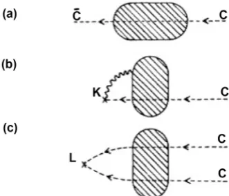
terms consist of everything but those parts of the propagator which are trans-verse in all indices. These terms give rise to unpleasant infinities already at the one-loop order. For example, the graviton self-energy diagram shown in Figure 4
has a divergent part with the general structure
( )
4 2h
∂ . Such divergences do cancel
when they are connected to tree diagrams whose outermost lines are on the mass shell, as they must if the S matrix is to be made finite without introducing
counterterms for them. However, they greatly complicate the renormalization of Green’s functions.
We may attempt to extricate ourselves from the situation described in the last paragraph by picking a different weighting functional. Keeping in mind that we want no part of the graviton propagator to fall off slower than p−4 for large
momenta, we now choose the weighting functional [14]
( )
1 4 24
1
exp d ,
2
eτ i xeτ eτ
ω = ∆−
∫
(96)where eτ is any four-vector function. The corresponding gauge-fixing term in
the effective action is
2 1 4 2
1
d .
2 xF F
τ τ
κ −
− ∆
∫
(97)The graviton propagator resulting from the gauge-fixing term (97) is derived in [14]. For most values of the parameters α and β in Isym it satisfies the
requirement that all its leading parts fall off like 4
p− for large momenta. There
are, however, specific choices of these parameters which must be avoided. If
0
α= , the massive spin-2 excitations disappear, and inspection of the graviton
propagator shows that some terms then behave like 2
k− . Likewise, if
3β α− =0, the massive scalar excitation disappears, and there are again terms
in the propagator which behave like p−2. However, even if we avoid the special
cases α=0 and 3β α− =0, and if we use the propagator derived from (97),
we still do not obtain a clean renormalization of the Green’s functions. We now turn to the implications of gauge invariance. Before we write down the BRS transformations for gravity, let us first establish the commutation relation for gravitational gauge transformations, which reveals the group structure of the theory. Take the gauge transformation (94) of hµν, generated by ξµ and