Models of Translation Competitions

Models of Translation Competitions

Mark Hopkins and Jonathan May

SDL Research

6060 Center Drive, Suite 150 Los Angeles, CA 90045

{mhopkins,jmay_}@sdl.com

Abstract

What do we want to learn from a trans-lation competition and how do we learn it with confidence? We argue that a dis-proportionate focus on ranking competi-tion participants has led to lots of differ-ent rankings, but little insight about which rankings we should trust. In response, we provide the first framework that allows an empirical comparison of different analy-ses of competition results. We then use this framework to compare several analyt-ical models on data from the Workshop on Machine Translation (WMT).

1 The WMT Translation Competition Every year, the Workshop on Machine Transla-tion (WMT) conducts a competiTransla-tion between ma-chine translation systems. The WMT organizers invite research groups to submit translation sys-tems in eight different tracks: Czech to/from En-glish, French to/from EnEn-glish, German to/from English, and Spanish to/from English.

For each track, the organizers also assemble a panel of judges, typically machine translation spe-cialists.1 _{The role of a judge is to repeatedly rank} five different translations of the same source text. Ties are permitted. In Table 1, we show an ex-ample2 _{where a judge (we’ll call him “jdoe”) has} ranked five translations of the French sentence “Il ne va pas.”

Each such elicitation encodes ten pairwise com-parisons, as shown in Table 2. For each compe-tition track, WMT typically elicits between 5000 and 20000 comparisons. Once the elicitation pro-cess is complete, WMT faces a large database of comparisons and a question that must be an-swered: whose system is the best?

1_{Although in recent competitions, some of the judging has}

also been crowdsourced (Callison-Burch et al., 2010).

2_{The example does not use actual system output.}

rank system translation 1 bbn “He does not go.” 2 (tie) uedin “He goes not.” 2 (tie) jhu “He did not go.”

4 cmu “He go not.”

5 kit “He not go.”

Table 1: WMT elicits preferences by asking judges to simultaneously rank five translations, with ties permitted. In this (fictional) example, the source sentence is the French “Il ne va pas.”

source text sys1 sys2 judge preference “Il ne va pas.” bbn cmu jdoe 1 “Il ne va pas.” bbn jhu jdoe 1 “Il ne va pas.” bbn kit jdoe 1 “Il ne va pas.” bbn uedin jdoe 1 “Il ne va pas.” cmu jhu jdoe 2 “Il ne va pas.” cmu kit jdoe 1 “Il ne va pas.” cmu uedin jdoe 2 “Il ne va pas.” jhu kit jdoe 1 “Il ne va pas.” jhu uedin jdoe 0 “Il ne va pas.” kit uedin jdoe 2

Table 2: Pairwise comparisons encoded by Ta-ble 1. A preference of 0 means neither translation was preferred. Otherwise the preference specifies the preferred system.

2 A Ranking Problem

For several years, WMT used the following heuris-tic for ranking the translation systems:

ORIGWMT(s) = win(s) +tie(s)

win(s) +tie(s) +loss(s)

For system s, win(s) is the number of pairwise

comparisons in which swas preferred, loss(s)is

the number of comparisons in whichswas

dispre-ferred, andtie(s)is the number of comparisons in

which sparticipated but neither system was

pre-ferred.

Recently, (Bojar et al., 2011) questioned the ad-equacy of this heuristic through the following

gument. Consider a competition with systemsA

andB. Suppose that the systems are different but

equally good, such that one third of the time A

is judged better than B, one third of the time B

is judged better thanA, and one third of the time

they are judged to be equal. The expected values of ORIGWMT(A) and ORIGWMT(B) are both

2/3, so the heuristic accurately judges the systems to be equivalently good. Suppose however that we had duplicatedB and had submitted it to the

competition a second time as systemC. SinceB

andC produce identical translations, they should

always tie with one another. The expected value of ORIGWMT(A) would not change, but the

ex-pected value of ORIGWMT(B) would increase to

5/6, buoyed by its ties with systemC.

This vulnerability prompted (Bojar et al., 2011) to offer the following revision:

BOJAR(s) = win(s)

win(s) +loss(s)

The following year, it was BOJAR’s turn to be

crit-icized, this time by (Lopez, 2012):

Superficially, this appears to be an im-provement....couldn’t a system still be penalized simply by being compared to [good systems] more frequently than its competitors? On the other hand, couldn’t a system be rewarded simply by being compared against a bad system more frequently than its competitors?

Lopez’s concern, while reasonable, is less obvi-ously damning than (Bojar et al., 2011)’s criti-cism of ORIGWMT. It depends on whether the

collected set of comparisons is small enough or biased enough to make the variance in competi-tion significant. While this hypothesis is plausi-ble, Lopez makes no attempt to verify it. Instead, he offers a ranking heuristic of his own, based on a Minimum Feedback Arc solver.

The proliferation of ranking heuristics contin-ued from there. The WMT 2012 organizers (Callison-Burch et al., 2012) took Lopez’s ranking scheme and provided a variant called Most Proba-ble Ranking. Then, noting some potential pitfalls with that, they created two more, called Monte Carlo Playoffs and Expected Wins. While one could raise philosophical objections about each of these, where would it end? Ultimately, the WMT 2012 findings presented five different rankings for

the English-German competition track, with no guidance about which ranking we should pay at-tention to. How can we know whether one rank-ing is better than other? Or is this even the right question to ask?

3 A Problem with Rankings

Suppose four systems participate in a translation competition. Three of these systems are extremely close in quality. We’ll call these close1, close2, andclose3. Nevertheless, close1 is very slightly better3_{thanclose2, andclose2is very slightly} bet-ter thanclose3. The fourth system, calledterrific, is a really terrific system that far exceeds the other three.

Now which is the better ranking?

terrific,close3,close1,close2 (1) close1,terrific,close2,close3 (2)

Spearman’s rho4_{would favor the second ranking,} since it is a less disruptive permutation of the gold ranking. But intuition favors the first. While its mistakes are minor, the second ranking makes the hard-to-forgive mistake of placingclose1ahead of theterrificsystem.

The problem is not with Spearman’s rho. The problem is the disconnnect between the knowl-edge that we want a ranking to reflect and the knowledge that a ranking actually contains. With-out this additional knowledge, we cannot deter-mine whether one ranking is better than another, even if we know the gold ranking. We need to determine what information they lack, and define more rigorously what we hope to learn from a translation competition.

4 From Rankings to Relative Ability Ostensibly the purpose of a translation competi-tion is to determine the relative ability of a set of translation systems. Let S be the space of all translation systems. Hereafter, we will refer toS

as the space ofstudents. We choose this term to evoke the metaphor of a translation competition as a standardized test, which shares the same goal: to assess the relative abilities of a set of participants. But what exactly do we mean by “ability”? Be-fore formally defining this term, first recognize that it means little without context, namely:

1. What kind of source text do we want the systems to translate well? Say system A is great at translating travel-related documents, but terrible at translating newswire. Mean-while, system B is pretty good at both. The question “which system is better?” requires us to state how much we care about travel versus newswire documents – otherwise the question is underspecified.

2. Who are we trying to impress? While it’s tempting to think that translation quality is a universal notion, the 50-60% interannota-tor agreement in WMT evaluations (Callison-Burch et al., 2012) suggests otherwise. It’s also easy to imagine reasons why one group of judges might have different priorities than another. Think a Fortune 500 company ver-sus web forum users. Lawyers verver-sus lay-men. Non-native versus native speakers. Posteditors versus Google Translate users. Different groups have different uses for trans-lation, and therefore different definitions of what “better” means.

With this in mind, let’s define some additional el-ements of a translation competition. LetX be the space of all possible segments of source text,J be

the space of all possible judges, andΠ ={0,1,2}

be the space of pairwise preferences.5 _We as-sume all spaces are countable. Unless stated oth-erwise, variabless1ands2represent students from S, variablex represents a segment fromX, vari-ablej represents a judge from _J, and variableπ

represents a preference fromΠ. Moreover, define thenegationπˆof preferenceπsuch thatπˆ = 2(if π= 1),ˆπ= 1(ifπ = 2), andπˆ = 0(ifπ= 0).

Now assume a joint distribution

P(s1, s2, x, j, π) specifying the probability

that we ask judge j to evaluate students s1 and s2’s respective translations of source text x, and

that judge j’s preference is π. We will further

assume that the choice of student pair, source text, and judge are marginally independent of one another. In other words:

P(s1, s2, x, j, π)

= P(π|s1, s2, x, j)·P(x|s1, s2, j) ·P(j_|s1, s2)·P(s1, s2)

= P(π_|s1, s2, x, j)·P(x)·P(j)·P(s1, s2) = P_X(x)_·P_J(j)_·P(s1, s2)·P(π|s1, s2, x, j)

5_{As a reminder, 0 indicates no preference.}

It will be useful to reserve notation P_X and P_J

for the marginal distributions over source text and judges. We can marginalize over the source seg-ments and judges to obtain a useful quantity:

P(π_|s1, s2)

= X

x∈X

X

j∈J

P_X(x)_·P_J(j)_·P(π_|s1, s2, x, j)

We refer to this as thehP_X, P_Ji-relative abilityof

students s1 ands2. By using different marginal

distributions P_X, we can specify what kinds of

source text interest us (for instance, P_X could

focus most of its probability mass on German tweets). Similarly, by using different marginal distributionsP_J, we can specify what judges we

want to impress (for instance,P_J could focus all

of its mass on one important corporate customer or evenly among all fluent bilingual speakers of a language pair).

With this machinery, we can express the pur-pose of a translation competition more clearly: to estimate thehP_X, P_Ji-relative ability of a set of students. In the case of WMT, P_J

presum-ably6 _{defines a space of competent} source-to-target bilingual speakers, whileP_X defines a space of newswire documents.

We’ll refer to an estimate of P(π_|s1, s2) as

a preference model. In other words, a prefer-ence model is a distribution Q(π_|s1, s2). Given

a set of pairwise comparisons (e.g., Table 2), the challenge is to estimate a preference model

Q(π_|s1, s2)such thatQis “close” toP. For

mea-suring distributional proximity, a natural choice is KL-divergence (Kullback and Leibler, 1951), but we cannot use it here becauseP is unknown.

Fortunately, if we have i.i.d. data drawn fromP,

then we can do the next best thing and compute the perplexity of preference modelQon this heldout test data. LetDbe a sequence of tripleshs1, s2, πi

where the preferences π are i.i.d. samples from P(π_|s1, s2). The perplexity of preference model Qon test dataDis:

perplexity(Q_|D) = 2−Phs1,s2,πi∈D|D|1 log2Q(π|s1,s2)

How do we obtain such a test set from competi-tion data? Recall that a WMT competicompeti-tion pro-duces pairwise comparisons like those in Table 2. 6_{One could argue that it specifies a space of machine}

Let C be the set of comparisons hs1, s2, x, j, πi

obtained from a translation competition. Com-petition data C is not necessarily7 sampled i.i.d.

fromP(s1, s2, x, j, π)because we may

intention-ally8_{bias data collection towards certain students,} judges or source text. Also, because WMT elicits its data in batches (see Table 1), every segmentx

of source text appears in at least ten comparisons. To create an appropriately-sized test set that closely resembles i.i.d. data, we isolate the sub-set C0 of comparisons whose source text appears

in at mostkcomparisons, wherekis the smallest

positive integer such that|C0_{|>= 2000. We then}

create the test setDfromC0:

D={hs1, s2, πi|hs1, s2, x, j, πi ∈ C0}

We reserve the remaining comparisons for training preference models. Table 3 shows the resulting dataset sizes for each competition track.

Unlike with raw rankings, the claim that one preference model is better than another has testable implications. Given two competing mod-els, we can train them on the same comparisons, and compare their perplexities on the test set. This gives us a quantitative9 _{answer to the question of} which is the better model. We can then publish a system ranking based on the most trustworthy preference model.

5 Baselines

Let’s begin then, and create some simple prefer-ence models to serve as baselines.

5.1 Uniform

The simplest preference model is a uniform distri-bution over preferences, for any choice of students

s1, s2:

Q(π|s1, s2) = 1

3 ∀π∈Π

This will be our only model that does not require training data, and its perplexity on any test set will be 3 (i.e. equal to number of possible preferences).

5.2 Adjusted Uniform

Now suppose we have a set C of comparisons available for training. Let Cπ ⊆ C denote the

subset of comparisons with preferenceπ, and let 7_{In WMT, it certainly is not.}

8_{To collect judge agreement statistics, for instance.} 9_{As opposed to philosophical.}

C(s1, s2)denote the subset comparing studentss1

ands2.

Perhaps the simplest thing we can do with the training data is to estimate the probability of ties (i.e. preference 0). We can then distribute the remaining probability mass uniformly among the other two preferences:

Q(π|s1, s2) =         

|C0|

|C| ifπ= 0 1₋|C0|

|C|

2 otherwise

6 Simple Bayesian Models

6.1 Independent Pairs

Another simple model is the direct estimation of each relative abilityP(π_|s1, s2)independently. In

other words, for each pair of studentss1ands2, we

estimate a separate preference distribution. The maximum likelihood estimate of each distribution would be:

Q(π|s1, s2) = |Cπ

(s1, s2)|+|Cπˆ(s2, s1)| |C(s1, s2)|+|C(s2, s1)|

However the maximum likelihood estimate would test poorly, since any zero probability estimates for test set preferences would result in infinite per-plexity. To make this model practical, we assume a symmetric Dirichlet prior with strengthαfor each

preference distribution. This gives us the follow-ing Bayesian estimate:

Q(π_|s1, s2) =

α+_|Cπ(s1, s2)|+|Cπˆ(s2, s1)| 3α+|C(s1, s2)|+|C(s2, s1)|

We call this the Independent Pairs preference model.

6.2 Independent Students

The Independent Pairs model makes a strong inde-pendence assumption. It assumes that even if we know that student A is much better than student B, and that student B is much better than student C, we can infer nothing about how student A will fare versus student C. Instead of directly estimating the relative abilityP(π_|s1, s2)of students s1 ands2,

we could instead try to estimate theuniversal abil-ity P(π|s1) = Ps2∈SP(π|s1, s2)·P(s2|s1) of each individual student s1 and then try to

preference distribution, which gives us the follow-ing Bayesian estimate:

Q(π|s1) =

α+P_s2∈S|Cπ(s1, s2)|+|Cˆπ(s2, s1)| 3α+P_s2∈S|C(s1, s2)|+|C(s2, s1)|

The estimatesQ(π_|s1)do not yet constitute a

pref-erence model. A downside of this approach is that there is no principled way to reconstruct a pref-erence model from the universal ability estimates. We experiment with three ad-hoc reconstructions. Theasymmetricreconstruction simply ignores any information we have about students2:

Q(π|s1, s2) =Q(π|s1)

The arithmetic and geometric reconstructions compute an arithmetic/geometric average of the two universal abilities:

Q(π|s1, s2) =

Q(π_|s1) +Q(ˆπ|s2) 2

Q(π_|s1, s2) = [Q(π|s1)∗Q(ˆπ|s2)]

1 2

We respectively call these the (Asymmet-ric/Arithmetic/Geometric) Independent Students preference models. Notice the similarities be-tween the universal ability estimatesQ(π_|s1)and

the BOJARranking heuristic. These three models

are our attempt to render the BOJAR heuristic as

preference models.

7 Item-Response Theoretic (IRT) Models Let’s revisit (Lopez, 2012)’s objection to the BO -JARranking heuristic: “...couldn’t a system still be

penalized simply by being compared to [good sys-tems] more frequently than its competitors?” The official WMT 2012 findings (Callison-Burch et al., 2012) echoes this concern in justifying the exclu-sion of reference translations from the 2012 com-petition:

[W]orkers have a very clear preference for reference translations, so includ-ing them unduly penalized systems that, through (un)luck of the draw, were pit-ted against the references more often.

Presuming the students are paired uniformly at random, this issue diminishes as more compar-isons are elicited. But preference elicitation is ex-pensive, so it makes sense to assess the relative ability of the students with as few elicitations as possible. Still, WMT 2012’s decision to eliminate

references entirely is a bit of a draconian mea-sure, a treatment of the symptom rather than the (perceived) disease. If our models cannot function in the presence of training data variation, then we should change the models, not the data. A model that only works when the students are all about the same level is not one we should rely on.

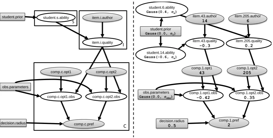
We experiment with a simple model that relaxes some independence assumptions made by previ-ous models, in order to allow training data vari-ation (e.g. who a student has been paired with) to influence the estimation of the student abili-ties. Figure 1(left) shows plate notation (Koller and Friedman, 2009) for the model’s indepen-dence structure. First, each student’sability dis-tribution is drawn from a common prior distribu-tion. Then a number of translationitemsare gen-erated. Eachitemisauthoredby a student and has a quality drawn from the student’s ability distri-bution. Then a number of pairwise comparisons are generated. Eachcomparisonhas twooptions, each a translationitem. Thequality of each item isobservedby a judge (possibly noisily) and then the judge states apreferenceby comparing the two observations.

We investigate two parameterizations of this model: Gaussian and categorical. Figure 1(right) shows an example of the Gaussian parameteriza-tion. The student ability distributions are Gaus-sians with a known standard deviationσa, drawn

from a zero-mean Gaussian prior with known stan-dard deviation σ0. In the example, we show

the ability distributions for students 6 (an above-average student, whose mean is 0.4) and 14 (a poor student, whose mean is -0.6). We also show an item authored by each student. Item 43 has a somewhat low quality of -0.3 (drawn from stu-dent 14’s ability distribution), while item 205 is not student 6’s best work (he produces a mean quality of 0.4), but still has a decent quality at 0.2. Comparison 1 pits these items against one another. A judge draws noise from a zero-mean Gaussian with known standard deviationσobs, then adds this

student.6.ability

Gauss(0.4, σa)

item.43.author 14

item.43.quality -0.3

comp.1.opt1 43

comp.1.opt1.obs -0.42

comp.1.pref 2

comp.1.opt2 205

comp.1.opt2.obs 0.35 student.prior

Gauss(0.0, σ0)

decision.radius 0.5 obs.parameters

Gauss(0.0, σobs)

item.205.author 6

item.205.quality 0.2 student.14.ability

Gauss(-0.6, σa) student.s.ability item.i.author

item.i.quality

comp.c.opt1

comp.c.opt1.obs

comp.c.pref

comp.c.opt2

comp.c.opt2.obs S

I

C

student.prior

decision.radius obs.parameters

Figure 1: Plate notation (left) showing the independence structure of the IRT Models. Example instan-tiated subnetwork (right) for the Gaussian parameterization. Shaded rectangles are hyperparameters. Shaded ellipses are variables observable from a set of comparisons.

radius (which here is 0.5), then he states no prefer-ence (i.e. a preferprefer-ence of 0). Otherwise he prefers the item with the higher observed quality.

The categorical parameterization is similar to the Gaussian parameterization, with the following differences. Item quality is not continuous, but rather a member of the discrete set {1,2, ...,Λ_}.

The student ability distributions are categorical distributions over {1,2, ...,Λ_}, and the student

ability prior is a symmetric Dirichlet with strength

αa. Finally, the observed quality is the item

qual-ity λ plus an integer-valued noise ν _{∈ {}1 ₋ λ, ...,Λ₋λ_}. Noiseνis drawn from a discretized

zero-mean Gaussian with standard deviationσobs.

Specifically,P r(ν)is proportional to the value of

the probability density function of the zero-mean GaussianN(0, σobs).

We estimated the model parameters with Gibbs sampling (Geman and Geman, 1984). We found that Gibbs sampling converged quickly and con-sistently10 _{for both parameterizations. Given the} parameter estimates, we obtain a preference model

Q(π_|s1, s2)through the inference query:

P r(comp.c0.pref=π _| item.i0.author=s1,

item.i00.author=s2,

comp.c0.opt1=i0,

comp.c0.opt2=i00)

10_{We ran 200 iterations with a burn-in of 50.}

where c0,i0,i00 are new comparison and item ids that do not appear in the training data.

We call these models Item-Response Theo-retic (IRT) models, to acknowledge their roots in the psychometrics (Thurstone, 1927; Bradley and Terry, 1952; Luce, 1959) and item-response theory (Hambleton, 1991; van der Linden and Hambleton, 1996; Baker, 2001) literature. Item-response theory is the basis of modern testing theory and drives adaptive standardized tests like the Graduate Record Exam (GRE). In particular, the Gaussian parameterization of our IRT models strongly resembles11 _{the Thurstone (Thurstone,} 1927) and Bradley-Terry-Luce (Bradley and Terry, 1952; Luce, 1959) models of paired compari-son and the 1PL normal-ogive and Rasch (Rasch, 1960) models of student testing. From the test-ing perspective, we can view each comparison as two students simultaneously posing a test question to the other: “Give me a translation of the source text which is better than mine.” The students can answer the question correctly, incorrectly, or they can provide a translation of analogous quality. An extra dimension of our models is judge noise, not a factor when modeling multiple-choice tests, for which the right answer is not subject to opinion.

11_{These models are not traditionally expressed using}

wmt10 wmt11 wmt12 lp train test train test train test

ce 3166 2209 1706 3216 5969 6806

fe 5918 2376 2556 4430 7982 5840

ge 7422 3002 3708 5371 8106 6032

se 8411 2896 1968 3684 3910 7376

ec 10490 3048 8859 9016 13770 9112

ef 5720 2242 3328 5758 7841 7508

eg 10852 2842 5964 7032 10210 7191

es 2962 2212 4768 6362 5664 8928

Table 3: Dataset sizes for each competition track (number of comparisons).

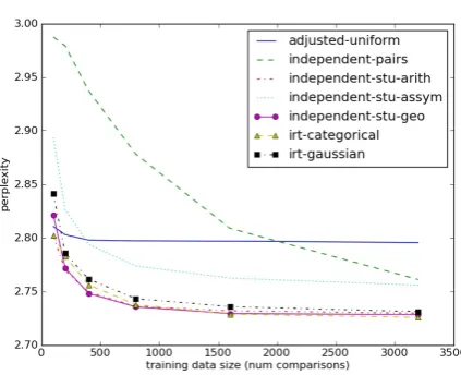
Figure 2: WMT10 model perplexities. The per-plexity of the uniform preference model is 3.0 for all training sizes.

8 Experiments

We organized the competition data as described at the end of Section 4. To compare the preference models, we did the following:

• Randomly chose a subset of k

compar-isons from the training set, for k _∈

{100,200,400,800,1600,3200_}.12

• Trained the preference model on these com-parisons.

• Evaluated the perplexity of the trained model

on the test preferences, as described in Sec-tion 4.

For each model and training size, we averaged the perplexities from 5 trials of each competition track. We then plotted average perplexity as a function of training size. These graphs are shown

12_{Ifkwas greater than the total number of training}

com-parisons, then we took the entire set.

Figure 3: WMT11 model perplexities.

Figure 4: WMT12 model perplexities.

in Figure 2 (WMT10)13_{, and Figure 4 (WMT12).} For WMT10 and WMT11, the best models were the IRT models, with the Gaussian parameteriza-tion converging the most rapidly and reaching the lowest perplexity. For WMT12, in which refer-ence translations were excluded from the compe-tition, four models were nearly indistinguishable: the two IRT models and the two averaged Indepen-dent StuIndepen-dent models. This somewhat validates the organizers’ decision to exclude the references, par-ticularly given WMT’s use of the BOJARranking

heuristic (the nucleus of the Independent Student models) for its official rankings.

13_{Results for WMT10 exclude the German-English and}

English-German tracks, since we used these to tune our model hyperparameters. These were set as follows. The Dirichlet strength for each baseline was 1. For IRT-Gaussian: σ0= 1.0, σobs= 1.0, σa= 0.5, and the decision radius was

0.4. For IRT-Categorical:Λ = 8, σobs= 1.0, αa= 0.5, and

Figure 6: English-Czech WMT11 results (average of 5 trainings on 1600 comparisons). Error bars (left) indicate one stddev of the estimated ability means. In the heatmap (right), cell(s1, s2)is darker if

preference modelQ(π_|s1, s2)skews in favor of students1, lighter if it skews in favor of students2.

Figure 5: WMT10 model perplexities (crowd-sourced versus expert training).

The IRT models proved the most robust at han-dling judge noise. We repeated the WMT10 ex-periment using the same test sets, but using the unfiltered crowdsourced comparisons (rather than “expert”14 _{comparisons) for training. Figure 5} shows the results. Whereas the crowdsourced noise considerably degraded the Geometric Inde-pendent Students model, the IRT models were re-markably robust. IRT-Gaussian in particular came close to replicating the performance of Geometric Independent Students trained on the much cleaner expert data. This is rather impressive, since the crowdsourced judges agree only 46.6% of the time, compared to a 65.8% agreement rate among

14_{I.e., machine translation specialists.}

expert judges (Callison-Burch et al., 2010). Another nice property of the IRT models is that they explicitly model student ability, so they yield a natural ranking. For training size 1600 of the WMT11 English-Czech track, Figure 6 (left) shows the mean student abilities learned by the IRT-Gaussian model. The error bars show one standard deviation of the ability means (recall that we performed 5 trials, each with a random training subset of size 1600). These results provide fur-ther insight into a case analyzed by (Lopez, 2012), which raised concern about the relative ordering ofonline-B, cu-bojar, and cu-marecek. Accord-ing to IRT-Gaussian’s analysis of the data, these three students are so close in ability that any order-ing is essentially arbitrary. Short of a full rankorder-ing, the analysis does suggest four strata. Viewing one of IRT-Gaussian’s induced preference models as a heatmap15_{(Figure 6, right), four bands are} dis-cernable. First, the reference sentences are clearly the darkest (best). Next come students 2-7, fol-lowed by the slightly lighter (weaker) students 8-10, followed by the lightest (weakest) student 11.

9 Conclusion

WMT has faced a crisis of confidence lately, with researchers raising (real and conjectured) issues with its analytical methodology. In this paper, we showed how WMT can restore confidence in

15_{In the heatmap, cell(s}

1, s2)is darker if preference model

Q(π_|s1, s2)skews in favor of students1, lighter if it skews

its conclusions – by shifting the focus from rank-ingstorelative ability. Estimates of relative ability (the expected head-to-head performance of system pairs over a probability space of judges and source text) can be empirically compared, granting sub-stance to previously nebulous questions like:

1. Is my analysis better than your analysis?

Rather than the current anecdotal approach to comparing competition analyses (e.g. pre-senting example rankings that seem some-how wrong), we can empirically compare the predictive power of the models on test data.

2. How much of an impact does judge noise have on my conclusions? We showed that judge noise can have a significant im-pact on the quality of our conclusions, if we use the wrong models. However, the IRT-Gaussian appears to be quite noise-tolerant, giving similar-quality conclusions on both expert and crowdsourced comparisons.

3. How many comparisons should I elicit?

Many of our preference models (including IRT-Gaussian and Geometric Independent Students) are close to convergence at around 1000 comparisons. This suggests that we can elicit far fewer comparisons and still derive confident conclusions. This is the first time a concrete answer to this question has been provided.

References

F.B. Baker. 2001. The basics of item response theory. ERIC.

Ondej Bojar, Miloˇs Ercegovˇcevi´c, Martin Popel, and Omar Zaidan. 2011. A grain of salt for the wmt manual evaluation. In Proceedings of the Sixth Workshop on Statistical Machine Translation, pages 1–11, Edinburgh, Scotland, July. Association for Computational Linguistics.

Ralph Allan Bradley and Milton E Terry. 1952. Rank analysis of incomplete block designs: I. the method of paired comparisons. Biometrika, 39(3/4):324– 345.

C. Callison-Burch, P. Koehn, C. Monz, K. Peterson, M. Przybocki, and O.F. Zaidan. 2010. Findings of the 2010 joint workshop on statistical machine trans-lation and metrics for machine transtrans-lation. In Pro-ceedings of the Joint Fifth Workshop on Statistical Machine Translation and MetricsMATR, pages 17– 53. Association for Computational Linguistics.

Chris Callison-Burch, Philipp Koehn, Christof Monz, Matt Post, Radu Soricut, and Lucia Specia. 2012. Findings of the 2012 workshop on statistical ma-chine translation. In Proceedings of the Seventh Workshop on Statistical Machine Translation. S. Geman and D. Geman. 1984. Stochastic relaxation,

gibbs distributions, and the bayesian restoration of images. IEEE Transactions on Pattern Analysis and Machine Intelligence, 6(6):721–741.

R.K. Hambleton. 1991. Fundamentals of item re-sponse theory, volume 2. Sage Publications, Incor-porated.

D. Koller and N. Friedman. 2009.Probabilistic graph-ical models: principles and techniques. MIT press.

S. Kullback and R.A. Leibler. 1951. On information and sufficiency. The Annals of Mathematical Statis-tics, 22(1):79–86.

Adam Lopez. 2012. Putting human assessments of machine translation systems in order. In Proceed-ings of WMT.

R. Ducan Luce. 1959. Individual Choice Behavior a Theoretical Analysis. John Wiley and sons.

R.J. Mislevy and R.G. Almond. 1997. Graphical mod-els and computerized adaptive testing. UCLA CSE Technical Report 434.

R.J. Mislevy, R.G. Almond, D. Yan, and L.S. Stein-berg. 1999. Bayes nets in educational assessment: Where the numbers come from. In Proceedings of the fifteenth conference on uncertainty in artifi-cial intelligence, pages 437–446. Morgan Kaufmann Publishers Inc.

G. Rasch. 1960. Studies in mathematical psychology: I. probabilistic models for some intelligence and at-tainment tests.

Louis L Thurstone. 1927. A law of comparative judg-ment.Psychological review, 34(4):273–286.