Evaluating Text Segmentation using Boundary Edit Distance
Chris Fournier
University of Ottawa Ottawa, ON, Canada
Abstract
This work proposes a new segmentation evaluation metric, named boundary simi-larity(B), an inter-coder agreement coef-ficient adaptation, and a confusion-matrix for segmentation that are all based upon an adaptation of the boundary edit distance in Fournier and Inkpen (2012). Existing seg-mentation metrics such as Pk,
WindowD-iff, and Segmentation Similarity (S) are all able to award partial credit for near misses between boundaries, but are biased towards segmentations containing few or tightly clustered boundaries. Despite S’s improvements, its normalization also pro-duces cosmetically high values that over-estimate agreement & performance, lead-ing this work to propose a solution.
1 Introduction
Text segmentation is the task of splitting text into segments by placing boundaries within it. Seg-mentation is performed for a variety of purposes and is often a pre-processing step in a larger task. E.g., text can be topically segmented to aid video and audio retrieval (Franz et al., 2007), question answering (Oh et al., 2007), subjectivity analysis (Stoyanov and Cardie, 2008), and even summa-rization (Haghighi and Vanderwende, 2009).
A variety of segmentation granularities, or atomic units, exist, including segmentations at the morpheme (e.g., Sirts and Alum¨ae 2012), word (e.g., Chang et al. 2008), sentence (e.g., Rey-nar and Ratnaparkhi 1997), and paragraph (e.g., Hearst 1997) levels. Between each atomic unit lies the potential to place a boundary. Segmentations can also represent the structure of text as being organized linearly (e.g., Hearst 1997), hierarchi-cally (e.g., Eisenstein 2009), etc. Theoretihierarchi-cally, segmentations could also contain varying
bound-ary types, e.g., two boundbound-ary types could differen-tiate between act and scene breaks in a play.
Because of its value to natural language pro-cessing, various text segmentation tasks have been automated such as topical segmentation— for which a variety of automatic segmenters exist (e.g., Hearst 1997, Malioutov and Barzilay 2006, Eisenstein and Barzilay 2008, and Kazantseva and Szpakowicz 2011). This work addresses how to best select an automatic segmenter and which seg-mentation metrics are most appropriate to do so.
To select an automatic segmenter for a particu-lar task, a variety of segmentation evaluation met-rics have been proposed, including Pk
(Beefer-man and Berger, 1999, pp. 198–200), WindowDiff (WD; Pevzner and Hearst 2002, p. 10), and most recently Segmentation Similarity (S; Fournier and Inkpen 2012, p. 154–156). Each of these met-rics have a variety of flaws: Pk and
WindowD-iff both under-penalize errors at the beginning of segmentations (Lamprier et al., 2007) and have a bias towards favouring segmentations with few or tightly-clustered boundaries (Niekrasz and Moore, 2010), while S produces overly optimistic values due to its normalization (shown later).
To overcome the flaws of existing text segmen-tation metrics, this work proposes a new series of metrics derived from an adaptation of boundary edit distance (Fournier and Inkpen, 2012, p. 154– 156). This new metric is namedboundary similar-ity(B). A confusion matrix to interpret segmenta-tion as a classificasegmenta-tion problem is also proposed, allowing for the computation of information re-trieval (IR) metrics such as precision and recall.1
In this work: §2 reviews existing segmentation metrics; §3 proposes an adaptation of boundary edit distance, a new normalization of it, a new confusion matrix for segmentation, and an
inter-1An implementation of boundary edit distance,
bound-ary similarity, B-precision, and B-recall, etc. is provided at http://nlp.chrisfournier.ca/
coder agreement coefficient adaptation; §4 com-pares existing segmentation metrics to those pro-posed herein; §5 evaluates S and B based inter-coder agreement; and §6 compares B, S, and WD while evaluating automatic segmenters.
2 Related Work
2.1 Segmentation Evaluation
Many early studies evaluated automatic seg-menters using information retrieval (IR) metrics such as precision, recall, etc. These metrics looked at segmentation as a binary classification prob-lem and were very harsh in their comparisons—no credit was awarded for nearly missing a boundary. Near misses occur frequently in segmentation— although manual coders often agree upon the bulk of where segment lie, they frequently disagree upon the exact position of boundaries (Artstein and Poesio, 2008, p. 40). To attempt to overcome this issue, both Passonneau and Litman (1993) and Hearst (1993) conflated multiple manual segmen-tations into one that contained only those bound-aries which the majority of coders agreed upon. IR metrics were then used to compare automatic seg-menters to this majority solution. Such a major-ity solution is unsuitable, however, because it does not contain actual subtopic breaks, but instead the conflation of a collection of potentially disagree-ing solutions. Additionally, the definition of what constitutes a majority is subjective (e.g., Passon-neau and Litman (1993, p. 150), Litman and Pas-sonneau (1995), Hearst (1993, p. 6) each used4/
7, 3/
7, and>50%, respectively).
To address the issue of awarding partial credit for an automatic segmenter nearly missing a boundary—without conflating segmentations, Beeferman and Berger (1999, pp. 198–200) pro-posed a new metric named Pk. Pevzner and Hearst
(2002, pp. 3–4) explain Pkwell: a window of size
k—where kis half of the mean manual
segmen-tation length—is slid across both automatic and manual segmentations. A penalty is awarded if the window’s edges are found to be in differing or the same segments within the manual segmen-tation and the automatic segmensegmen-tation disagrees. Pkis the sum of these penalties over all windows.
Measuring the proportion of windows in error al-lows Pk to penalize a fully missed boundary by
kwindows, whereas a nearly missed boundary is
penalized by the distance that it is offset.
Pk was not without issue, however. Pevzner
and Hearst (2002, pp. 5–10) identified that Pk:
i) penalizes false negatives (FNs)2more than false
positives (FPs); ii) does not penalize full misses withinkunits of a reference boundary; iii) penal-ize near misses too harshly in some situations; and iv) is sensitive to internal segment size variance.
To solve Pk’s issues, Pevzner and Hearst (2002,
pp. 10) proposed a modification referred to as WindowDiff (WD). Its major difference is in how it decides to penalized windows: within a window, if the number of boundaries in the manual segmen-tation (Mij) differs from the number of
bound-aries in the automatic segmentation (Aij), then a
penalty is given. The ratio of penalties over win-dows then represents the degree of error between the segmentations, as in Equation 1. This change better allowed WD to: i) penalize FPs and FNs more equally;3 ii) Not skip full misses; iii) Less
harshly penalize near misses; and iv) Reduce its sensitivity to internal segment size variance.
WD(M, A) = 1
N−k
NX−k
i=1,j=i+k
(|Mij−Aij|>0) (1)
WD did not, however, solve all of the issues related to window-based segmentation compari-son. WD, and inherently Pk: i) Penalize
er-rors less at the beginning and end of segmenta-tions (Lamprier et al., 2007); ii) Are biased to-wards favouring automatic segmentations with ei-ther few or tightly-clustered boundaries (Niekrasz and Moore, 2010); iii) Calculate window size k
inconsistently;4 iv) Are not symmetric5 (meaning
that they cannot be used to produce a pairwise mean of multiple manual segmentations6).
Segmentation Similarity (S; Fournier and Inkpen 2012, pp. 154–156) took a different ap-proach to comparing segmentations. Instead of us-ing windows, the work proposes a new restricted edit distance calledboundary edit distancewhich differentiates between full and near misses. S then
2I.e., a boundary present in the manual but not the
auto-matic segmentation, and the reverse for a false positive.
3Georgescul et al. (2006, p. 48) noted that WD interprets
a near miss as a FP probabilistically more than as a FN.
4kmust be an integer, but half of a mean may be a
frac-tion, thus rounding must be used, but no rounding method is specified. It is also not specified whetherkshould be set once during a study or recalculated for each comparison— this work assumes the latter.
5Window size is calculated only upon the manual
segmen-tation, meaning that one must be a manual and other an auto-matic segmentation.
6This also means that WD and P
k cannot be adapted to
normalizes the counts of full and near misses iden-tified by boundary edit distance, as shown in Equa-tion 2, wheresa andsb are the segmentations,nt
is the maximum distance that boundaries may span to be considered a near miss, edits(sa, sb, nt)is the
edit distance, and pb(D)is the number of potential
boundaries in a documentD(pb(D) =|D| −1).
S(sa, sb, nt) = 1−|edits
(sa, sb, nt)|
pb(D) (2)
Boundary edit distance models full misses as the addition/deletion of a boundary, and near misses asn-wise transpositions. Ann-wise
trans-position is the act of swapping the trans-position of a boundary with an empty position such that it matches a boundary in the segmentation compared against (up to a spanning distance of nt). S also
scales the severity of a near miss by the distance over which it is transposed, allowing it to scale the penalty of a near misses much like WD. S is also symmetric, allowing it to be used in pairwise means and inter-coder agreement coefficients.
The usage of an edit distance that supported transpositions to compare segmentations was an advancement over window-based methods, but boundary edit distance and its normalization S are not without problems, specifically: i) This edit dis-tance uses string reversals (ABCD =⇒ DCBA) to perform transpositions, making it cumbersome to analyse individual pairs of boundaries between segmentations; ii) S is sensitive to variations in the total size of a segmentation, leading it to favour very sparse segmentations with few boundaries; iii) S produces cosmetically high values, making it difficult to interpret and causing over-estimation of inter-coder agreement. In this work, these defi-ciencies are demonstrated and a new set of metrics are proposed as replacements.
2.2 Inter-Coder Agreement
Inter-coder agreement coefficients are used to measure whether a group of human judges (i.e. coders) agree with each other greater than chance. Such coefficients are used to determine the relia-bility and replicarelia-bility of the coding scheme and instructions used to collect manual codings (Car-letta, 1996). Although direct interpretation of such coefficients is difficult, they are an invaluable tool when comparing segmentation data that has been collected with differing labels and when estimat-ing the replicability of a study. A variety of
inter-coder agreement coefficients exist, but this work focuses upon a selection of those discussed by Art-stein and Poesio (2008), specifically: Scott’s π
(Scott, 1955) Fleiss’ multi-π (π∗, Fleiss 1971)7,
Cohen’sκ(Cohen, 1960), and multi-κ(κ∗, Davies
and Fleiss 1982). Their general forms are shown in Equation 3, where Aarepresents actual agreement,
and Aeexpected (i.e., chance) agreement between
coders.
κ, π, κ∗, andπ∗ = Aa−Ae
1−Ae (3)
When calculating agreement between manual segmenters, boundaries are considered labels and their positions the decisions. Unfortunately, be-cause of the frequency of near misses that oc-cur in segmentation, using such labels and de-cisions causes inter-coder agreement coefficients to drastically underestimate actual agreement— much like how automatic segmenter performance is underestimated when segmentation is treated as a binary classification problem. Hearst (1997, pp. 53–54) attempted to adapt π∗ to award
par-tial credit for near misses by using the percentage agreement metric of Gale et al. (1992, p. 254) to compute actual agreement—which conflates mul-tiple manual segmentations together according to whether a majority of coders agree upon a bound-ary or not. Unfortunately, such a method of com-puting agreement grossly inflates results, and “the statistic itself guarantees at least 50% agreement by only pairing off coders against the majority opinion” (Isard and Carletta, 1995, p. 63).
Fournier and Inkpen (2012, pp. 154–156) pro-posed using pairwise mean S for actual agree-ment to allow inter-coder agreeagree-ment coefficients to award partial credit for near misses. Unfor-tunately, because S produces cosmetically high values, it also causes inter-coder agreement coef-ficients to drastically overestimates actual agree-ment. This work demonstrates this deficiency and proposes and evaluates a solution.
3 A New Proposal for Edit-Based Text Segmentation Evaluation
In this section, a new boundary edit distance based segmentation metric and confusion matrix is pro-posed to solve the deficiencies of S for both seg-mentation comparison and inter-coder agreement.
3.1 Boundary Edit Distance
In this section, Boundary Edit Distance (BED; as proposed in Fournier and Inkpen 2012, pp. 154– 156) is introduced in more detail, and a few termi-nological and conceptual changes are made.
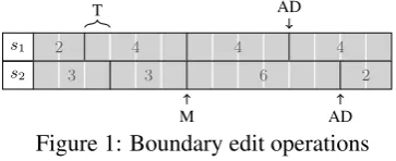
Boundary Edit Distance uses three main edit op-erations to model segmentation differences:
• Additions/deletions (AD; referred to origi-nally as substitutions) for full misses; • Substitutions (S; not shown for brevity) for
confusing one boundary type with another; • n-wise transpositions (T) for near misses.
These edit operations are symmetric and oper-ate upon the set of boundaries that occur at each potential boundary position in a pair of segmenta-tions. An example of how these edit operations are applied8 is shown in Figure 1, where a near miss
(T), a matching pair of boundaries (M), and two full misses (ADs) are shown with the maximum distance that a transposition can span (nt) set to 2
potential boundaries (i.e., only adjacent positions can be transposed).
s1 22 44 44 44
s2 33 33 66 22
T
M
AD
[image:4.595.334.495.102.153.2]AD
Figure 1: Boundary edit operations In Figure 1, the location of the errors is clearly shown. Importantly, however, pairs of boundaries between the segmentations can be seen that rep-resent the decisions made, and the correctness of these decisions. Imagine thats1 is a manual
seg-mentation, ands2is an automatic segmenter’s
hy-pothesis. The transposition is a partially correct decision, or boundary pair. The match is a correct boundary pair. The additions/deletions, however, could be one of two erroneous decisions: to not place an expected boundary (FN), or to place a su-perfluous boundary (FP).9
This work proposes assigning a correctness score for each boundary pair/decision (shown in Table 1) and then using the mean of this score as a normalization of boundary edit distance. This interpretation intuitively relates boundary edit dis-tance to coder judgements, making it ideal for
8A complete explanation of Boundary Edit Distance is
de-tailed in Fournier (2013, Section 4.1.2).
9Also note that the ADs are close together, and ifn t>2,
then they would be considered a T, and not two ADs—this is one way to award partial credit for near misses.
calculating actual agreement in inter-coder agree-ment coefficients and comparing segagree-mentations.
Pair Correctness
Match 1
Addition/deletion 0
Transposition 1−wt span(Te, nt)
Substitution 1−ws ord(Se,Tb)
Table 1: Correctness of boundary pair
3.2 Boundary Similarity
The new boundary edit distance normalization proposed herein is referred to asboundary similar-ity(B). Assuming that boundary edit distance pro-duces sets of edit operations where Aeis the set of
additions/deletions, Te the set of n-wise
transpo-sitions, Sethe set of substitutions, and BM the set
of matching boundary pairs, boundary similarity similarity can be defined as shown in Equation 4— one minus the incorrectness of each boundary pair over the total number of boundary pairs.
B(s1, s2, nt) = 1−|Ae|
+wt span(Te, nt) +ws ord(Se,Tb)
|Ae|+|Te|+|Se|+|BM|
(4)
This form, one minus a penalty function, was chosen so that it was easier to compare against other penalty functions considered (not shown here for brevity). This normalization was also cho-sen because it is equivalent to mean boundary pair correctness and so that it ranges in value from 0 to 1. In the worst case, a segmentation comparison will result in no matches, no near misses, no sub-stitutions, andXfull misses, i.e.,|Ae|=Xand all
other terms in Equation 4 are zero, meaning that:
B= 1− X+ 0 + 0
X+ 0 + 0 + 0 = 1−X/X= 1−1 = 0
In the best case, a segmentation comparison will result in X matches, no near misses, no substitu-tions, and no full misses, i.e.,|BM| = X and all
other terms in Equation 4 are zero, meaning that:
B= 1− 0 + 0 + 0 0 + 0 + 0 +X
= 1−0/X= 1−0 = 1
For all other scenarios, varying numbers of matches, near misses, substitutions and full misses will result in values of B between 0 and 1.
Equation 4 takes two segmentations (in any or-der), and the maximum transposition spanning distance (nt). This distance represents the
[image:4.595.88.270.386.460.2]the severity of a near miss. A variety of scaling functions could be used, and this work arbitrarily chooses a simple fraction to represent each trans-position’s severity in terms of its distance from its paired boundary overntplus a constantwt(0 by
default), as shown in Equation 5.
wt span(Te, nt) = |Te| X
j=1
wt+abs
(Te[j][1]−Te[j][2])
nt−1
(5)
If multiple boundary types are used, then sub-stitution edit operations would occur when one boundary type was confused with another. As-signing each boundary type tb ∈ Tb a number on
an ordinal scale, substitutions can be weighted by their distance on this scale over the maximum dis-tance plus a constantws (0 by default), as shown
in Equation 6.
ws ord(Se,Tb) = |Se| X
j=1
ws+abs
(Se[j][1]−Se[j][2])
max(Tb)−min(Tb)
(6)
These scaling functions allow for edit penalties to range from 0 tows/tplus some linear distance. 3.3 A Confusion Matrix for Segmentation
The mean correctness of each pair (i.e., B) gives an indication of just how similar one segmentation is to another, but what if one wants to identify some specific attributes of the performance of an auto-matic segmenter? Is the segmenter confusing one boundary type with another, or is it very precise but has poor recall? The answers to these ques-tions can be obtained by looking at text segmenta-tion as a multi-class classificasegmenta-tion problem.
This work proposes using a task’s set of bound-ary types (Tb) and the lack of a boundary (∅)
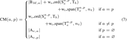
to represent the set of segmentation classes in a boundary classification problem. Using these classes, a confusion matrix (defined in Equation 7) can be created which sums boundary pair correct-ness so that information-retrieval metrics can be calculated that award partial credit to near misses by scaling edits operations.
CM(a, p) =
|BM,a|+wsord(Sa,pe ,Tb)
+wtspan(Ta,pe , nt) ifa=p
wsord(Sa,pe ,Tb)
+wtspan(Ta,p
e , nt) ifa6=p
|Ae,a| ifp=∅
|Ae,p| ifa=∅
(7)
An example confusion matrix is shown in Fig-ure 2 from which IR metrics such as precision, re-call, and Fβ-measure can be computed (referred to
as B-precision, B-recall, etc.).
Actual
Pr
edicted
B Non-B
B CM(1,1) CM(∅,1)
[image:5.595.333.512.57.103.2]Non-B CM(1,∅) CM(∅,∅)
Figure 2: Example confusion matrix (Tb={1})
3.4 B-Based Inter-coder Agreement
Fournier and Inkpen (2012, p. 156–157) adapted four inter-coder agreement formulations provided by Artstein and Poesio (2008) to use S to award partial credit for near misses, but because S pro-duces cosmetically high agreement values they grossly overestimate agreement. To solve this issue, this work instead proposes using micro-average B (i.e., mean boundary pair correctness over all documents and codings compared) to solve this issue (demonstrated in §5) because it does not over-estimate actual agreement (demon-strated in §4 and 5).
4 Discussion of Segmentation Metrics Before analysing how each metric compares to each other upon a large data set, it would be useful to investigate how they act on a smaller scale. To that end, this section discusses how each metric in-terprets a set of hypothetical segmentations of an excerpt of a poem by Coleridge (1816, pp. 55–58) titled Kubla Khan (shown in Figure 3)—chosen ar-bitrarily for its brevity (and beauty). These seg-mentations are topical and at the line-level.
1. In Xanadu did Kubla Khan 2. A stately pleasure-dome decree: 3. Where Alph, the sacred river, ran 4. Through caverns measureless to man 5. Down to a sunless sea.
6. So twice five miles of fertile ground 7. With walls and towers were girdled round: 8. And here were gardens bright with sinuous rills, 9. Where blossomed many an incense-bearing tree; 10. And here were forests ancient as the hills, 11. Enfolding sunny spots of greenery.
Figure 3: Excerpt from the poem Kubla Khan (Co-leridge, 1816, pp. 55–58) with line numbers
[image:5.595.80.291.642.709.2]contrived automatic segmentations are compared to this manual segmentation to illustrate how each metric reacts to different mistakes.
Lines Description
1–2 Kubla Khan and his decree 3–5 Waterways
6–11 Fertile ground and greenery
Figure 4: A hypothetical manual segmentation
Assuming that Figure 4 represents an accept-able manual segmentation (m), how would each
metric react to an automatic segmentation (a) that
combines the segments 1–2 and 3–5 together? This would represent a full miss, or a false neg-ative, as shown in Figure 5. S interprets these seg-mentations as being quite similar, yet, the auto-matic segmentation is missing a boundary. B and
1−W D,10in this case, better reflect this error.
m a
S B 1−W D
0.9 0.5 0.77¯7
[image:6.595.310.514.209.254.2]k= 2
Figure 5: False negative
How would each metric react to an automatic segmentation that is very close to placing the boundaries correctly, but makes the slight mis-take of thinking that the segment on waterways (3–5) ends a bit too early? This would repre-sent a near miss, as shown in Figure 6. S and
1−W D incorrectly interpret this error as being
equivalent to the previous false negative—a trou-bling result. Segmentation comparison metrics should be able to discern between the full and a near miss shown in these two figures, and an au-tomatic segmenter that nearly misses a boundary should be awarded a better score than one which fully misses a boundary—B recognizes this and awards the near miss a higher score.
m a
S B 1−W D 0.9 0.75 0.77¯7
[image:6.595.76.277.316.360.2]k= 2
Figure 6: Near miss
How would each metric react to an automatic segmentation that adds an additional boundary be-tween line 8 and 9? This would not be ideal because such a boundary falls in the middle of a cohesive description of a garden, representing
10WD is reported as1−W D because WD is normally a
penalty metric where a value of 0 is ideal, unlike S and B. Ad-ditionally,k= 2for all examples in this section because WD computeskfrom the manual segmentationm, which does not change in these examples.
a full miss, or false positive, as in Figure 7. S and1−W D incorrectly interpret this error as
be-ing equivalent to the previous two errors—an even more troubling result. In this case, there are two matching boundaries and a pair that do not match, which is arguably preferable to the full miss and one match in Figure 5, but not to the match and near miss in Figure 6. B recognizes this, and awards a higher score to this automatic segmenter than that in Figure 5, but below Figure 6.
m a
S B 1−W D 0.9 0.66¯6 0.77¯7
k= 2
Figure 7: False positive
How would each metric react to an automatic segmentation that compensates for its lack of pre-cision by spuriously adding boundaries in clusters around where it thinks that segments should begin or end? This is shown in Figure 8. This kind of behaviour is finally penalized differently by S and
1−W D(unlike the other errors shown in this
sec-tion), but it only barely results in a dip in their val-ues. B also penalizes this behaviour, but does so much more harshly—in B’s interpretation, this is as egregious as committing a false negative (e.g., Figure 5)—an arguably correct interpretation, if the evaluation desires to maximize similarity with a manual segmentation.
m a
S B 1−W D
0.8 0.5 0.66¯6
[image:6.595.311.516.464.504.2]k= 2
Figure 8: Cluster of false positives These short demonstrations of how S, B, and
1−W D interpret error should lead one to con-clude that: i) WD can penalize near misses to the same degree as full misses—overly harshly; ii) Both S and WD are not very discriminating when small segments are analysed; and iii) B is the only one of the three metrics that is able to often discriminate between these situations. B, if used to rank these automatic segmenters, would rank them from best to worst performing as: the near miss, false positive, and then a tie between the false negative and cluster of false positives—a reasonable ranking in the context of an evaluation seeking similarity with a manual segmentation.
5 Segmentation Agreement
[image:6.595.75.281.584.629.2]sec-0.0 0.1 0.2 0.3 0.4 0.5 0.6 0.7 0.8 P(miss) while P(near) = 0.0921
0.75 0.80 0.85 0.90 0.95 1.00
π
−
value
using
S
2 3 4
5 6 7
8 9 10
(a) S-based π∗ showing increasing full
misses with constant near misses
0.0 0.1 0.2 0.3 0.4 0.5 0.6 0.7 0.8 P(miss) while P(near) = 0.0921
0.2 0.4 0.6 0.8 1.0
π
−
value
using
Bb
2 3 4
5 6 7
8 9 10
(b) B-based π∗ showing increasing full
misses with constant near misses
2 3 4 5 6 7 8 9 10
Coders (quantity) 0.0
0.2 0.4 0.6 0.8 1.0
π
−
value
using
Bb
S B
(c) S and B basedπ∗with fully random
[image:7.595.78.522.61.160.2]segmentations
Figure 9: Artificial data sets illustrating how π adapted to use either S or B reacts to increasing full
misses and random segmentations and varying numbers of coders
tion, it makes sense to analyse some larger data sets. Two such data sets are The Stargazer data set collected by Hearst (1997) and The Moonstone data set collected by Kazantseva and Szpakowicz (2012). Both are linear topical segmentations at the paragraph level with only one boundary type, but that is where their similarities end.
The Stargazer text is a science magazine article titled “Stargazers look for life” (Baker, 1990) seg-mented by 7 coders and was one of twelve articles chosen for its length (between 1,800 and 2,500 words) and for having little structural demarca-tion. “The Moonstone” is a 19thcentury romance
novel by Collins (1868) segmented by 4–6 coders per chapter; of its 23 chapters, 2 were coded in a pilot study and another 20 were coded individually by 27 undergraduate English students in 5 groups. For the Stargazer data set, using S-based π∗,
an inter-coder agreement coefficient of0.7562is
obtained—a reasonable level by content analysis standards. Unfortunately, this value is highly in-flated, and B-basedπ∗ gives a much more
conser-vative coefficient at 0.4405. For the Moonstone
data set, the agreement coefficients for each group of 4–6 coders using S-based π∗ is again
over-inflated at 0.91, 0.92, 0.90, 0.94, 0.83. B-based
π∗ instead reports that the coefficients should be
0.20, 0.18, 0.40, 0.38, 0.23.
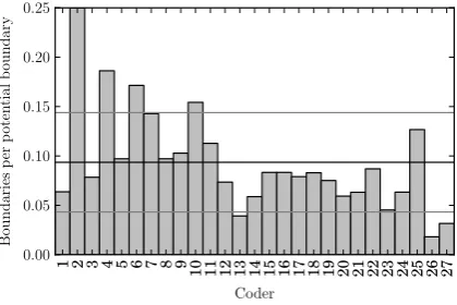
Which of these coefficients should be trusted? Is agreement in these data sets high or low? To help answer that, this work looks at how the coders in the data sets behaved. If the segmenters in the Moonstone data set truly agreed with each other, then they should have all behaved similarly. One measure of coder behaviour is the frequency that they placed boundaries (normalized by their op-portunity to place boundaries, i.e. the sum of the potential boundaries in the chapters that each seg-mented). This normalized frequency is shown per
1 2 3 4 5 6 7 8 9 10 11 12 13 14 15 16 17 18 19 20 21 22 23 24 25 26 27 Coder
0.00 0.05 0.10 0.15 0.20 0.25
Boundaries
p
er
p
oten
tial
b
oundary
Figure 11: Normalized boundaries placed by each coder in the Moonstone data set (with mean±SD)
coder in Figure 11 for The Moonstone data set, along with bars indicating the mean and one stan-dard deviation above and below. As can be seen, the coders fluctuated wildly in the frequency with which they placed boundaries—some (e.g., coder 7) to degrees exceeding 2 standard deviations. The Moonstone data set as a whole does not exhibit coders who behaved similarly, supporting the as-sertion by B-based π∗ that these coders do not
[image:7.595.312.522.238.378.2]declin-Random Human BayesSeg APS MinCut Automatic segmenter
0.80 0.82 0.84 0.86 0.88 0.90 0.92 0.94
S
−
value
n= 90 n= 90 n= 90 n= 90 n= 90
(a) S
Random Human BayesSeg APS MinCut Artificial Segmenter
0.2 0.3 0.4 0.5 0.6
Bb
mean
and
95%
CIs
n= 1057 n= 841 n= 964 n= 738 n= 871
(b) B
Random Human BayesSeg APS MinCut Automatic segmenter
0.35 0.40 0.45 0.50 0.55 0.60 0.65 0.70 0.75
1
−
W
D
−
value
n= 90 n= 90 n= 90 n= 90 n= 90
(c)1−W D
Figure 10: Mean performance of 5 segmenters using varying metrics with 95% confidence intervals
ing amount of agreement which is unaffected by the number of pseudo-coders. This is not appar-ent, however, for S-basedπ∗ in Figure 9a; as the
probability of a full miss increases, agreement ap-pears to rise and varies depending upon the num-ber of pseudo-coders. B-basedπ∗however shows
declining agreement and little to no variation de-pending upon the number of pseudo-coders, as shown in Figure 9b.
If instead of creating pseudo-coders from a ran-dom segmentation a series of ranran-dom segmenta-tions with the same parameters were generated, a properly functioning inter-coder agreement coef-ficient should report some agreement (due to the similar parameters used to create the segmenta-tions) but it should be quite low. Figure 9c shows this, and that S-basedπ∗drastically over-estimates what should be very low agreement whereas B-basedπ∗properly reports low agreement.
From these demonstrations, it is evident that S-based inter-coder agreement coefficients dras-tically over-estimate agreement, as does S itself in pairwise mean form. B-based coefficients, however, properly discriminate between levels of agreement regardless of the number of coders and do not over-estimate.
6 Evaluation of Automatic Segmenters
Having looked at how S, WD, and B perform at a small scale in §4 and on larger data set in §5, this section demonstrates the use of these met-rics to evaluate some automatic segmenters. Three automatic segmenters were trained—or had their parameters estimated upon—The Moonstone data set, including MinCut; (Malioutov and Barzilay, 2006), BayesSeg; (Eisenstein and Barzilay, 2008), and APS (Kazantseva and Szpakowicz, 2011).
To put this evaluation into context, an upper and lower bound were also created comprised of a ran-dom coder from the manual data (Human) and a
random segmenter (Random), respectively. These automatic segmenters, and the upper and lower bounds, were created, trained, and run by another researcher (Anna Kazantseva) with their labels re-moved during the development of the metrics de-tailed herein (to improve the impartiality of these analyses). An ideal segmentation evaluation met-ric should, in theory, place the three automatic seg-menters between the upper and lower bounds in terms of performance if the metrics, and the seg-menters, function properly.
The mean performance of the upper and lower bounds upon the test set of the Moonstone data set using S, B, and WD are shown in Figure 10a– 10c along with 95% confidence intervals. Despite the difference in the scale of their values, both S and WD performed almost identically, placing the three automatic segmenters between the upper and lower bounds as expected. For S, statistically sig-nificant differences11 (α = 0.05) were found
be-tween all segmenters except bebe-tween APS–human and MinCut–BayesSeg, and WD could only find significant differences between the automatic seg-menters and the upper and lower bounds. B, how-ever, shows a marked deviation, and places Min-Cut and APS statistically significantly below the random baseline with only BayesSeg between the upper and lower bounds—to a significant degree.
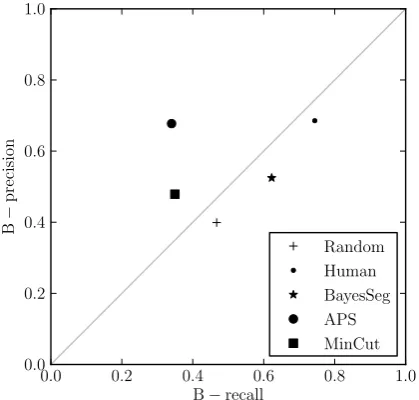
Why would pairwise mean B act in such an unexpected manner? The answer lies in a fur-ther analysis using the confusion matrix proposed earlier to calculate B-precision and B-recall (as shown in Table 2). From the values in Table 2, all three automatic segmenters appear to have B-precision above the baseline and below the upper bound, but the B-recall of both APS and MinCut is below that of the random baseline (illustrated
11Using Kruskal-Wallis rank sum multiple comparison
B n B-P B-R B-F1 TP FP FN TN Random 0.2640±0.0129 1057 0.3991 0.4673 0.4306 279.0 420 318 4236.0
[image:9.595.119.487.62.124.2]Human 0.5285±0.0164 841 0.6854 0.7439 0.7135 444.5 204 153 4451.5 BayesSeg 0.3745±0.0146 964 0.5247 0.6224 0.5694 361.0 327 219 4346.0 APS 0.2873±0.0163 738 0.6773 0.3403 0.4530 212.0 101 411 4529.0 MinCut 0.2468±0.0141 871 0.4788 0.3496 0.4041 215.0 234 400 4404.0
Table 2: Mean performance of 5 segmenters using micro-average B, B-precision (B-P), B-recall (B-R), and B-Fβ-measure (B-F1) along with the associated confusion matrix values for 5 segmenters
0.0 0.2 0.4 0.6 0.8 1.0
B−recall 0.0
0.2 0.4 0.6 0.8 1.0
B
−
precision
Random Human BayesSeg APS MinCut
Figure 12: Mean B-precision versus B-recall of 5 automatic segmenters
in Figure 12). These automatic segmenters were developed and performance tuned using WD, thus it would be expected that they would perform as they did according to WD, but the evaluation using B highlights WD’s bias towards sparse segmenta-tions (i.e., those with low B-recall)—a failing that S also appears to share. Mean B shows an un-biased ranking of these automatic segmenters in terms of the upper and lower bounds. B, then, should be preferred over S and WD for an un-biased segmentation evaluation that assumes that similarity to a human solution is the best measure of performance for a task.
7 Conclusions
In this work, a new segmentation evaluation met-ric, referred to as boundary similarity (B) is proposed as an unbiased metric, along with a boundary-edit-distance-based (BED-based) con-fusion matrix to compute predictably biased IR metrics such as precision and recall. Additionally, a method of adapting inter-coder agreement coef-ficients to award partial credit for near misses is proposed that uses B as opposed to S for actual agreement so as to not over-estimate agreement.
B overcomes the cosmetically high values of S and, the bias towards segmentations with few or tightly-clustered boundaries of WD–manifesting in this work as a bias towards precision over recall for both WD and S. When such precision is desir-able, however, B-precision can be computed from a BED-based confusion matrix, along with other IR metrics. WD and Pk should not be preferred
because their biases do not occur consistently in all scenarios, whereas BED-based IR metrics offer expected biases built upon a consistent, edit-based, interpretation of segmentation error.
B also allows for an intuitive comparison of boundary pairs between segmentations, as op-posed to the window counts of WD or the sim-plistic edit count normalization of S. When an un-biased segmentation evaluation metric is desired, this work recommends the usage of B and the use of an upper and lower bound to provide context. Otherwise, if the evaluation of a segmentation task requires some biased measure, the predictable bias of IR metrics computed from a BED-based con-fusion matrix is recommended. For all evalua-tions, however, a justification for the biased/un-biased metrics used should be given, and more than one metric should be reported so as to allow a reader to ascertain for themselves whether a par-ticular automatic segmenter’s bias in some manner is cause for concern or not.
8 Future Work
Future work includes adapting this work to anal-yse hierarchical segmentations and using it to at-tempt to explain the low inter-coder agreement co-efficients reported in topical segmentation tasks.
Acknowledgements
[image:9.595.76.286.174.374.2]References
Artstein, Ron and Massimo Poesio. 2008. Inter-coder agreement for computational linguistics.
Computational Linguistics34(4):555–596. Baker, David. 1990. Stargazers look for life.South
Magazine117:76–77.
Beeferman, Doug and Adam Berger. 1999. Sta-tistical models for text segmentation. Machine Learning34:177–210.
Carletta, Jean. 1996. Assessing Agreement on Classification Tasks: The Kappa Statistic. Com-putational Linguistics22(2):249–254.
Chang, Pi-Chuan, Michel Galley, and Christo-pher D. Manning. 2008. Optimizing Chinese word segmentation for machine translation per-formance. In Proceedings of the Third Work-shop on Statistical Machine Translation. Asso-ciation for Computational Linguistics, Strouds-burg, PA, USA, pages 224–232.
Cohen, Jacob. 1960. A Coefficient of Agreement for Nominal Scales. Educational and Psycho-logical Measurement20:37–46.
Coleridge, Samuel Taylor. 1816. Christabel, Kubla Khan, and the Pains of Sleep. John Mur-ray.
Collins, Wilkie. 1868. The Moonstone. Tinsley Brothers.
Davies, Mark and Joseph L. Fleiss. 1982. Measur-ing agreement for multinomial data. Biometrics
38:1047–1051.
Eisenstein, Jacob. 2009. Hierarchical text seg-mentation from multi-scale lexical cohesion. InProceedings of Human Language Technolo-gies: The 2009 Annual Conference of the North American Chapter of the Association for Com-putational Linguistics. Association for Com-putational Linguistics, Stroudsburg, PA, USA, pages 353–361.
Eisenstein, Jacob and Regina Barzilay. 2008. Bayesian unsupervised topic segmentation. In
Proceedings of the 2008 Conference on Em-pirical Methods in Natural Language Process-ing. Association for Computational Linguistics, Morristown, NJ, USA, pages 334–343.
Fleiss, Joseph L. 1971. Measuring nominal scale agreement among many raters. Psychological Bulletin76:378–382.
Fournier, Chris and Diana Inkpen. 2012. Segmen-tation Similarity and Agreement. In Proceed-ings of Human Language Technologies: The 2012 Annual Conference of the North American Chapter of the Association for Computational Linguistics. Association for Computational Lin-guistics, Stroudsburg, PA, USA, pages 152– 161.
Fournier, Christopher. 2013. Evaluating Text Seg-mentation. Master’s thesis, University of Ot-tawa.
Franz, Martin, J. Scott McCarley, and Jian-Ming Xu. 2007. User-oriented text segmentation eval-uation measure. InProceedings of the 30th An-nual International ACM SIGIR Conference on Research and Development in Information Re-trieval. Association for Computing Machinery, Stroudsburg, PA, USA, pages 701–702.
Gale, William, Kenneth Ward Church, and David Yarowsky. 1992. Estimating upper and lower bounds on the performance of word-sense dis-ambiguation programs. In Proceedings of the 30th Annual Meeting of the Association for Computational Linguistics. Association for Computational Linguistics, Stroudsburg, PA, USA, pages 249–256.
Georgescul, Maria, Alexander Clark, and Susan Armstrong. 2006. An analysis of quantita-tive aspects in the evaluation of thematic seg-mentation algorithms. In Proceedings of the 7th SIGdial Workshop on Discourse and Dia-logue. Association for Computational Linguis-tics, Stroudsburg, PA, USA, pages 144–151. Haghighi, Aria and Lucy Vanderwende. 2009.
Exploring content models for multi-document summarization. InProceedings of Human Lan-guage Technologies: The 2009 Annual Confer-ence of the North American Chapter of the As-sociation for Computational Linguistics. Asso-ciation for Computational Linguistics, Strouds-burg, PA, USA, NAACL ’09, pages 362–370. Hearst, Marti A. 1993. TextTiling: A Quantitative
Approach to Discourse. Technical report, Uni-versity of California at Berkeley, Berkeley, CA, USA.
Hearst, Marti A. 1997. TextTiling: Segmenting Text into Multi-paragraph Subtopic Passages.
Computational Linguistics23:33–64.
Nonparametric Statistical Methods. John Wi-ley & Sons, 2nd edition.
Isard, Amy and Jean Carletta. 1995. Replicability of transaction and action coding in the map task corpus. InAAAI Spring Symposium: Empirical Methods in Discourse Interpretation and Gen-eration. pages 60–66.
Kazantseva, Anna and Stan Szpakowicz. 2011. Linear Text Segmentation Using Affinity Prop-agation. InProceedings of the 2011 Conference on Empirical Methods in Natural Language Processing. Association for Computational Lin-guistics, Edinburgh, Scotland, UK., pages 284– 293.
Kazantseva, Anna and Stan Szpakowicz. 2012. Topical Segmentation: a Study of Human Per-formance. InProceedings of Human Language Technologies: The 2012 Annual Conference of the North American Chapter of the Asso-ciation for Computational Linguistics. Associ-ation for ComputAssoci-ational Linguistics, Strouds-burg, PA, USA, pages 211–220.
Lamprier, Sylvain, Tassadit Amghar, Bernard Levrat, and Frederic Saubion. 2007. On evuation methodologies for text segmentation al-gorithms. In Proceedings of the 19th IEEE In-ternational Conference on Tools with Artificial Intelligence. IEEE Computer Society, Washing-ton, DC, USA, volume 2, pages 19–26.
Litman, Diane J. and Rebecca J. Passonneau. 1995. Combining multiple knowledge sources for discourse segmentation. In Proceedings of the 33rd Annual Meeting of the Association for Computational Linguistics. Association for Computational Linguistics, Stroudsburg, PA, USA, pages 108–115.
Malioutov, Igor and Regina Barzilay. 2006. Min-imum cut model for spoken lecture segmen-tation. In Proceedings of the 21st Interna-tional Conference on ComputaInterna-tional Linguis-tics and the 44th annual meeting of the Asso-ciation for Computational Linguistics. Associ-ation for ComputAssoci-ational Linguistics, Strouds-burg, PA, USA, pages 25–32.
Niekrasz, John and Johanna D. Moore. 2010. Un-biased discourse segmentation evaluation. In
Proceedings of the IEEE Spoken Language Technology Workshop, SLT 2010. IEEE 2010, pages 43–48.
Oh, Hyo-Jung, Sung Hyon Myaeng, and Myung-Gil Jang. 2007. Semantic passage segmentation based on sentence topics for question answer-ing. Information Sciences177(18):3696–3717. Passonneau, Rebecca J. and Diane J. Litman.
1993. Intention-based segmentation: human reliability and correlation with linguistic cues. In Proceedings of the 31st Annual Meeting of the Association for Computational Linguis-tics. Association for Computational Linguistics, Stroudsburg, PA, USA, pages 148–155.
Pevzner, Lev and Marti A. Hearst. 2002. A cri-tique and improvement of an evaluation metric for text segmentation. Computational Linguis-tics28:19–36.
Reynar, Jeffrey C. and Adwait Ratnaparkhi. 1997. A maximum entropy approach to identifying sentence boundaries. In Proceedings of the 5th Conference on Applied Natural Language Processing. Association for Computational Lin-guistics, Stroudsburg, PA, USA, pages 16–19. Scott, William A. 1955. Reliability of content
analysis: The case of nominal scale coding.
Public Opinion Quarterly19:321–325.
Siegel, Sidney and N. J. Castellan. 1988. Non-parametric Statistics for the Behavioral Sci-ences, McGraw-Hill, New York, USA, chapter 9.8. 2nd edition.
Sirts, Kairit and Tanel Alum¨ae. 2012. A Hierar-chical Dirichlet Process Model for Joint Part-of-Speech and Morphology Induction. In Proceed-ings of Human Language Technologies: The 2012 Annual Conference of the North American Chapter of the Association for Computational Linguistics. Association for Computational Lin-guistics, Stroudsburg, PA, USA, pages 407– 416.