Solving a Large Real-world Bus Driver Scheduling
Problem with a Multi-assignment based Heuristic
Algorithm
Ademir Aparecido Constantino
(Universidade Estadual de Maring´a, Maring´a, Brazil [email protected])
Candido Ferreira Xavier de Mendon¸ca Neto (Universidade Estadual de S˜ao Paulo, S˜ao Paulo, Brazil
Silvio Alexandre de Araujo
(Universidade Estadual Paulista, S˜ao Jos´e do Rio Preto, Brazil [email protected])
Dario Landa-Silva
(University of Nottingham, Nottingham, UK [email protected])
Rog´erio Calvi
(Universidade Estadual def Maring´a, Maring´a, Brazil [email protected])
Allainclair Flausino dos Santos
(Universidade Estadual de Maring´a, Maring´a, Brazil [email protected])
Abstract: The bus driver scheduling problem (BDSP) under study consists in find-ing a set of duties that covers the bus schedule from a Brazilian public transportation bus company with the objective of minimizing the total cost. A deterministic 2-phase heuristic algorithm is proposed using multiple assignment problems that arise from a model based on a weighted multipartite graph. In the first phase, the algorithm con-structs an initial feasible solution by solving a number of assignment problems. In the second phase, the algorithm attempts to improve the solution by two different proce-dures. One procedure takes the whole set of duties and divides them in a set of partial duties which are recombined. The other procedure seeks to improve single long duties by eliminating the overtime time and inserting it into another duty. Computational tests are performed using large-scale real-world data with more than 2,300 tasks and random instances extracted from real data. Three different objective functions are an-alyzed. The overall results indicate that the proposed approach is competitive to solve large BDSP.
Key Words: bus driver scheduling, crew management, heuristic, transportation, large real-world instances.
1
Introduction
The Bus Driver Scheduling Problem (BDSP), or more generally named as the Crew Scheduling Problem (CSP) in transportation context, consists basically in generating a work schedule for a crew subject to a number of constraints and aiming to optimize a given objective function. This problem is known to be NP-hard and it has been extensively investigated as reported in the operational re-search literature since 1960’s. Several approaches were revised (e.g. [Bodin et al., 1983, Wren and Rousseau, 1995, Wren and Wren, 1995, Beasley and Chu, 1996]) and the progress of new developments have being reported in a series of spe-cialized workshops [Daduna and Wren, 1988]. A good summary of this devel-opment has been presented in the international workshops on Computer-Aided Scheduling of Public Transport (in 2009 this title was changed to “Conference of Advanced Systems of Public Transport” - CASPT) [CASPT2015, 2015].
The Crew Rostering Problem (CRP) and the Crew Scheduling Problem (CSP) are related problems that arise in crew management of large transporta-tion companies [Vera Valdes, 2010, Ernst et al., 2004]. Although the problems are related, usually CRP and CSP are solved separately and sequentially. Where the Crew scheduling is related to construct of shifts for a short period of time, e.g. for a day. In this phase the shifts are not yet assigned to individual crews. The crew rostering is a second phase in crew management in which the shifts generated during the crew scheduling phase are sequenced in order to form a roster for each crew for a larger planning horizon (typically a week or a month). The main focus of crew scheduling is the cost reduction, whilst the main focus of crew rostering is more related to aspects such as quality of life, rather than related to costs [Vera Valdes, 2010].
Despite these heuristic techniques, we found exact approaches based on the column generation (CG) technique to solve two real-world instances, both with up to 246 tasks [Yunes et al., 2005]. Their objective is to minimize the number of bus drivers instead of minimizing the total cost. Thus, they consider the unicost set covering (all columns have the same cost equal to one). Others researchers have investigated the CG technique (e.g., [Fores, 2001, Santos and Mateus, 2007, Shijun Chen, 2013, Li et al., 2015]). Recently [Shijun Chen, 2013] presented an improved CG algorithm which was applied to a set of real problem instances with up to 701 trips1.
A few papers have reported the use of a combination of CG with other approaches to solve the BDSP, e.g., [Santos and Mateus, 2007] reports the use of CG combined with Genetic Algorithm to solve instances with up to 138 tasks and [Li et al., 2015] reports the use of a CG based hyper-heuristic to solve real instances with 500 tasks.
Differently of the SCP or the SPP, a new mathematical formulation of the BDSP under special constraints imposed by Italian transportation rules was presented by [De Leone et al., 2011a]. Unfortunately, this formulation could only be useful when applied to small or medium-sized instances (up to 136 tasks). [De Leone et al., 2011a, De Leone et al., 2011b] report the use of a Greedy Randomized Adaptive Search Procedure (GRASP) that may be applied to larger instances. However, it can be applied to instances with at most 161 tasks.
Although most papers found in the literature report methods that use the SCP or the SPP to solve the BDSP, some studies use heuristics/meta-heuristics without using the SCP or the SPP. For example: the HACS algorithm that uses a tabu search [Shen and Kwan, 2001]; an evolutionary algorithm combined with fuzzy logic [Li and Kwan, 2003], a heuristic method, namely ZEST, derived from the process of manual scheduling [Liping Zhao, 2006]; a hybrid heuristic that combines GRASP and Rollout meta-heuristics to solve instances with 250 tasks [D’Annibale et al., 2007]; an algorithm based on Variable Neighborhood Search (VNS) to solve instances with 501 tasks [Ma et al., 2016]; an algorithm based on Iterated Local Search (ILS) [Silva and Reis, 2014] which is similar with VNS and Very Large-scale Neighborhood Search (VLNS); and a Self-Adjusting algorithm, based on evolutionary approach [Li, 2005].
Some papers report approaches that consider the scheduling of crews and the scheduling of vehicles simultaneously (or integratedly), trying to solve both problems at the same time. However, the computational time has been a criti-cal issue. For example: a combination of CG and Lagrangian relaxation which solves instances randomly generated as well as real-world data instances in which the number of tasks varies between 194 and 653 trips [Huisman et al., 2005]; a
GRASP based algorithm were applied to real-world instances with up to 249 tasks [Laurent and Hao, 2008], a set partition/covering-based approaches were applied to instances with up to 400 tasks [Mesquita and Paias, 2008]; and an integrated approach to solve real-world instances with up to 653 trips [De Groot and Huisman, 2008].
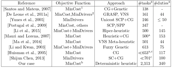
Table 1:Summary of the literature review comparing different features
Reference Objective Function Approach #tasks3#duties3 [Santos and Mateus, 2007] MinCost1 CG+Genetic 138
-[De Leone et al., 2011a] MinCost,MinDrivers2 GRASP, VNS 161 44 [Yunes et al., 2005] MinDrivers Unicost SCP+CG 246 ≤50 [Portugal et al., 2009] MinCost, others SCP/SPP 347
-[Li et al., 2015] MinCost+MinDrivers Hiper-heuristic 500 145 [Mauri and Lorena, 2007] MinCost Heuristic+CG 500a 153 [Ma et al., 2016] MinCost VNS Meta-heuristic 501 44 [Li and Kwan, 2003] MinCost+MinDrivers Fuzzy Genetic 613 75
[Huisman et al., 2005] MinCost CG 653a,c 117
[Shijun Chen, 2013] MinDrivers SC+CG 701c 100
Our case MinCostb Deterministic heuristic 2,313 340
1MinCost means minimizing the total cost.
2MinDriversmeans minimizing the number of drivers.
3#tasks e #duties means the number of tasks and duties respectively. aset of artificial benchmark instances.
bincluding vehicle changes and others functions are investigated. cnumber of trips (the number of tasks is not provided).
Some approachesfocus on the bus lines, i.e. the set of tasks is divided accord-ing to each bus line. Thus, the problem instance size is clearly reduced and solved separately (e.g. [Yunes et al., 2005]). However, [Portugal et al., 2009] reports an approach thatfocus on the network, i.e. the set of tasks is not divided according to each bus line and each task can be assigned to any driver despite the bus line it belongs to. In the work reported here we follow this approach. The set of tasks arises from 55 different bus lines and, due to the planning strategy of the company, are not separated. This means that a driver can drive in different bus lines during his/her daily duty. The company desires to minimize the number of bus line changes during a daily duty. Thus, this information is incorporated in our objective function as detailed in Section 3.
and an improvement phase. To the best of our knowledge this is the first time this approach is applied to solve a BDSP. We applied GraphBDSP with real-world problem instances from a Brazilian transportation bus company with 55 bus lines and more than 2,300 tasks, with about 340 duties and with two depots. In order to compare our results against the results reported in the literature we summarize our bibliography review in terms of instance sizes, features and approaches (see Table 1). According to our review, our problem instance is four times larger than the largest problem instance reported in the literature. Since we are dealing with a NP-hard problem spending a high computational effort to solve smaller instances, as reported, we belive that a heuristic technique can be justified to obtain good quality feasible solutions. The main advantages of the GraphBDSP are its effectiveness, its efficiency (low asymptotic complexity) and its facility in terms of parameter tuning.
In this context, this paper makes three contributions. The first contribution is the proposition of a new heuristic approach to solve a huge BDSP instance. Further, to the best of our knowledge, no paper considers this same set of labor rules (constraints and objective function). Also, it is worth noticing that this algorithm requires only one parameter to tune due to the simplicity of the crite-rion defined by [Cordeau et al., 2002]. The second contribution in this paper is to make available those new problem instances in order to promote new researches around this subject, including a large real-word problem instance. To the best of our knowledge, no paper deals with more than 500 tasks by exact approach. The third contribution is the application of three different objective functions which are compared, concluding that is more important to focus on idle time and overtime time instead of focusing on paid time only.
This paper is organized as follows. Section 2 gives the problem description. Section 3 presents the GraphBDSP in detail. Section 5 reports the computational results of GraphBDSP compared with set covering methods, giving lower bounds. Finally, Section 6 presents the conclusion remarks.
2
The Bus Driver Scheduling Problem
Terminology
Below we report some terminology used in this paper:
– Ablock represents a sequence of trips to be operated in a day by a vehicle from the time it leaves the depot (garage or the place were it is parked) until it returns to the same depot. These blocks are results from the vehicle scheduling2.
– A relief opportunity is a pair of place and time, into a block, in which a driver is allowed to leave or assume a vehicle.
– Ataskis a work defined by two consecutive relief opportunity and represents the minimum portion of work that can be assigned to a driver. Thus a task may involve one or more trips, usually two trips, or a deadhead3.
– Abus line is a route (itinerary) over which a bus regularly travels, although it is possible to use a bus in different lines.
– A running table is part of a block when the bus is used over the same line. Each row of a running table containing four entries which represents atask
t. These entries are defined byt= (sl, st, el, et), the first two entries indicate where and when the task starts the next two entries indicate where and when it ends, respectively. The information of which bus line a task t belongs is given bybl(t) and the values of each entry of the taskt is given by sl(t),
st(t),el(t) andet(t), respectively.
– A crew is a team of a driver and a conductor, but in some cases it may consists of a driver only. When weassigna crew to a taskt, that means that the crew is running the corresponding bus line from the placesl and timest
to the placeeland timeet.
– Apiece of work(POW) is a sequence of consecutive tasksti,ti+1, ...,tj, in the same bus line, assigned to the same crew whereet(tk)≤st(tk+1). – Astretch is a sequence of consecutive pieces of work (not necessarily in the
same bus line) without an intervening meal-break (rest time). Note that, by definition, a POW is a stretch and a single task is a POW. A POW (or a stretch )P = (ti, ti+1, ..., tj) starts at the same location (resp. time) where (resp. when) its first task starts. Thus,sl(P) = sl(ti) and st(P) = st(ti). Also, it ends at the same location (resp. time) where (resp when) its last task ends. Thus,el(P) =el(tj) andet(P) =et(tj).
2 We assume that the vehicle blocks is determined a priori by solving the vehicle scheduling. In this case we used the solutions provided by the public transport com-pany.
– There are two types of breaks:
• a rest time (rest break, meal-break) which is an unpaid time between two task assigned consecutively to the same driver; and
• aidle time(idle break) which is also a time between two tasks assigned consecutively to the same crew, however, idle time is a paid time used to complete a duty.
– AdutyD is an ordered sequence of tasks t1,t2, ...,tk (composed of one or more stretches) that can be assigned to a crew in a single day work.
– Aspreadover time(given bysot) of a dutyDis the time between the start of the first task ofDand the end of the last task ofD,sot(D) =et(tk)−st(t1). In this work, when we assign a task t to the end of a duty D, the task is always assigned to the same crew of duty D forming a new sequence where the tasktwill be in the last position. Therefore, for simplicity we say that we assign tasktto the end of dutyD.
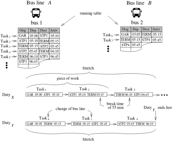
Figure 1 shows two bus linesAandB. Each bus line consists of a set of four entry columns where each row indicates all the tasks a bus must perform in a day (bus 1 and bus 2 for line A and bus 4, bus 5 and bus 6 for line B). This figure also shows two duties:
The DutyX where the first 3 tasks of the duty are Task1, Task2 and Task5. Note that, the first two tasks of the duty forms a POW and there is a rest time between Task2 and Task5; and
The DutyY where the first 3 tasks of the duty are Task6, Task3 and Task4. The whole duty consists of these 3 tasks, therefore, the crew will have a 367 minutes of idle time to complete their day work. Note that the crew assigned to this duty must change the bus line between Task6 Task3. Thus these 3 tasks forms a stretch .
2.1 Problem Specification
A feasible duty must meet the company regulations and the specific Brazilian legal restrictions established by both law and contracts with labor unions as follows.
Rule 1: The stretch time on a duty may not exceed 360 minutes, and if it exceeds this time, a rest time of at least 90 minutes must be applied. Rest time on a duty (unpaid time) may not exceed 300 minutes, otherwise the break time over that is considered idle time (paid time).
piece of work Stretch 5
Task Task4
3 Task Task2
1 Task
Bus line B
bus 2
Orig Dep Dest Arriv GAR 05:05 05:15
05:15 05:45 05:45
TERM
Task7 6 Task
STP4
TERM STP4
bus 1 Bus line A
Orig Dep Dest Arriv GAR 05:00 STP1 05:10 STP1 05:10TERM05:15 TERM 05:15 STP2
STP205:45TERM 06:10 05:45
TERM 06:10 STP3 STP3
06:45 06:45
running table
Stretch
6 3
GAR 05:05 TERM 05:15 TERM 05:15 STP2 05:45
Duty ends here
Task Task Task4
change of bus line Y
STP2 05:45 TERM 06:10
1 2 5
GAR 05:00 STP1 05:10
Duty
Task Task
Duty
Task
Y
X STP1 05:10 TERM 05:15 TERM 06:10 STP3 06:45
[image:8.595.152.447.109.354.2]of 55 min break time
Figure 1:Two bus lines showing a lists of tasks and two duties.
Rule 3: If a duty includesnight working, between 10pm and 5am, a period of 52 minutes is considered to be 60 minutes of work (called night time) and an additional payment of 20% of ordinary wage must be applied over such night working time. For overtime (extra working time) an additional payment of 50% of ordinary wage must be applied.
Rule 4: The total paid time per duty must be at least 432 minutes.
Rule 5: The spreadover time of a duty may not exceed 780 minutes.
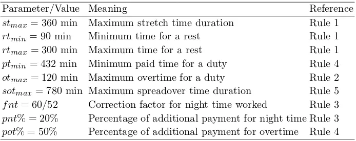
Table 2:Parameter notation from the problem.
Parameter/Value Meaning Reference
stmax= 360 min Maximum stretch time duration Rule 1 rtmin= 90 min Minimum time for a rest Rule 1 rtmax= 300 min Maximum time for a rest Rule 1 ptmin= 432 min Minimum paid time for a duty Rule 4 otmax= 120 min Maximum overtime for a duty Rule 2 sotmax= 780 min Maximum spreadover time duration Rule 5 f nt= 60/52 Correction factor for night time worked Rule 3
pnt% = 20% Percentage of additional payment for night time Rule 3
pot% = 50% Percentage of additional payment for overtime Rule 4
3
Proposed Algorithms
The proposed algorithm GraphBDSP is based on sucessive solution of (linear) assignment problems in order to construct and to improve diferent paths (duties) in a multipartite graph. The assignment problem [Pentico, 2007] is a well-known problem in operation research and it can be solved in polynomial time. The assignment problem has been quite used due to its low computational complex-ity to get optimal solution, e.g. recently it was sucessely used to takle a nurse scheduling problem [Constantino et al., 2014]. Given a cost matrix [cij] of di-mension n×n, the assignment problem consists in associating each row to a column in such a way that the total cost of the assignment is minimized. Using a binary variable xij = 1 if row i is associated with column j, the assignment problem can be formulated as follows:
min n
i=1 n
j=1
cijxij (1)
Subject to: n
i=1
xij= 1, j= 1, . . . , n (2) n
j=1
xij= 1, i= 1, . . . , n (3)
xij∈ {0,1}, i, j= 1, . . . , n (4)
where the number n and the cost matrix [cij] have different meaning (values) for each phase of the algorithm, which are explained in detail in the following sections.
3.1 Data and Solution Representation
First of all our algorithm starts with a weighted multipartite directed graph
G= (T, E) (or simply a graph) whereT is the set of verticesrepresenting the tasks the whose crews must be allocated and E is the set ofedgeseij = (ti, tj) indicating that the same crew can perform the tasktj after the taskti. In this case we say that ti isadjacent with tj and that eij leaves vertex ti and enters vertextj.
It is possible to place the set of vertices into layers T1, T2, ..., Tk (T =
∪k
m=1Tm) such that all edges are “forward”, i.e. for each edge eij = (ti, tj), vertexti is placed on layerTl and vertextj is placed on layerTm wherem > l. The vertices are arranged into layers in such way that each layers is made up of vertices representing tasks, if two tasks can be scheduled one after other, then they are not in the same layer, i.e. if tasktj can be scheduled after the task ti, then ti ∈ Tl and tj ∈ Tm, l < m. A simple greedy algorithm can build such partition. Letsm denote the size of the layerTm(1≤m≤k).
Let a path D = (T, A) be a sequence (v1, v2, ..., vu) of vertices of G such that vp is adjacent with vp+1 (1 ≤ p ≤ u−1). Its easy to show that a path meets each layer at most once. Two paths Dr and Ds are disjoint if and only if Dr∩Ds =∅. In the reminder of this work, we will refer to the vertices of Gas tasks and refer to the paths constructed by the algorithm as duties. Thus our algorithm try to find a set of disjoint paths (duties) that meets all vertices (tasks) of the graph (a partition ofT) minimizing the total cost. A solution is this set of disjoint paths.
Let a partial duty be an incomplete duty, this means that it is possible to include more task to obtain a complete duty. A partial duty is always referred with two indexes were the second index indicates the context of that part. Thus, a complete duty (or simply a duty) is referred with a single index. For example, we useDi to refer to a dutyito be carried out by a crew in a single day which can be split into two partial duties Dl
i,m−1 (called left partial duty) and Dri,m (called right partial duty), where Dl
i,m−1 contain the tasks ti,1, ti,2, ..., ti,m−1 andDr
i,m contain the tasksti,m,ti,m+1, ...,ti,k.
Our graph is edge-weighted graphs but the weight of each edge is computed dynamically. Since the additional cost of adding a task to a partial duty, or joining two partial duties, may not depend only on the last task of the partial dutyDl
3.2 Cost Function
Let λ-cost be a function that receives two parameters: a partial duty Dl i,m−1 and a partial duty Dr
j,m and returns the cost (related to paid time in minutes) of assigning the duty Dr
j,m at the end of dutyDli,m−1 forming the duty Di. If Di isfeasibletheλ-cost function returns the paid time in minutes; otherwise it returns∞(if it isunfeasible). Theλ-costfunction is defined in equation 5.
λ(Di,ml −1, Drj,m) = 5
r=1
λr (5)
whereλr is defined according to the set of rules stated in Section 2.1: Rule 1: Let bt(Di) = maxuk−=11{(st(ti,u+1)−et(ti,u))|((et(ti,u)−st(Di)) ≤
stmax)∧((et(Di)−st(ti,u+1))≤stmax)} be the longest break time of the duty Di which is candidate to be a rest time. If sot(Di) ≤ stmax we set α= 0; otherwise we setα=∞. Letrt(Di) be the rest time of the duty Di, i.e.rt(Di) =min{bt(Di), rtmax, α}. If rt(Di) = 0 or rt(Di)≥rtmim we set λ1= 0, otherwise we setλ1=∞.
Rule 2: Letotday(Di) and otnight(Di) be the overtime worked during the day and night (between 10pm and 5pm), respectively. Thus,ot(Di) =otday(Di)+ otday(Di)·f nt%. Ifot(Di)≤otmaxwe setλ2= 0, otherwise we setλ2 =∞. Rule 3: Letwt(Di) be the amount of working time of the dutyDi, i.e.wt(Di) = min{sot(Di)−rt(Di), ptmin}. Letnt(Di) be the amount of night time worked and let pt(Di) be the amount of paid time of the duty Di, i.e. pt(Di) = (wt(Di)−nt(Di)) + (nt(Di)·(1 +pnt%)) + (ot(Di)·pot%). Thus we set λ3=pt(Di).
Rule 4: Ifpt(Di)≥ptmin we setλ4= 0, otherwise we setλ4=∞. Rule 5: Ifot(Di)≤otmax we setλ5= 0, otherwise we setλ5=∞.
Aδ-penaltyfunction is defined as the value of a quantified penalty to reflect the bus line change and the feasibility of join Dl
i,m−1 to Dj,mr . The δ-penalty function is defined in equation 6.
δ(Dli,m−1, Dj,mr ) =δ1+δ2 (6) whereδ1 andδ2are computed as follows:
a)Letvc(Di) be the number of bus line change in Di, thus we set δ1= (pblc· vc(Di)), wherepblcis a penalty for a bus line change.
b)δ2 = 0 is (et(Dl
We define a cost function f which receives as parameter a pair of partial dutiesDli,m−1andDrj,mand returns the cost of assigning all tasks of the partial duty Dl
i,m−1 at the end of the partial duty Drj,m. In this work, we investigate three versions as follows:
f1(Dli,m−1,Dj,mr ) =λ(Dli,m−1, Drj,m) +δ(Di,ml −1,Drj,m), i.e. the in functionf1 only considers the paid time of assigning the partial dutyDl
i,m−1 at the end of the partial dutyDr
j,m.
f2(Dli,m−1,Drj,m) = (λ(Dli,m−1, Dj,mr )−λ3)+δ(Dli,m−1,Dj,mr )+it(Dli,m−1, Dj,mr ), whereit(Dl
i,m−1, Dj,mr ) returns the total idle time of the duty. This function focuses on idle time (paid break time) of the duty.
f3(Dli,m−1,Drj,m) = (λ(Dli,m−1, Dj,mr )−λ3)+δ(Dli,m−1,Dj,mr )+it(Dli,m−1, Dj,mr ) + (ot(Di)·pot%). This function focuses on idle time (paid break time) and overtime.
LetDbe the set of duties kept by the algorithm in a given time (the current solution). The cost f associated withD is given byf(D) =i|D=1|f(Di), where f can bef1,f2 orf3. These functions return∞ifDisunfeasible.
3.3 Construction Phase
In the construction phase a feasible schedule is built, i.e., a set of feasible du-ties, adding one task at a time according to a assignment problem, until all tasks have been assigned. Starting with an empty duties, iteratively each duty is constructed.
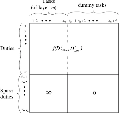
Let d be the number of estimated duties needed to assign all tasks, thus, it must be enough to assign the tasks to one of the d partial duties. We used
d= 2.5nv, wherenvis the number of vehicles obtained by the vehicle scheduling. We definedummy tasktas a not real task and there is no restriction to assign it to any partial duty at any release opportunity without changing any cost or property. In addition, sl(t) = el(t) = N U LL, st(t) = et(t) = 0. But since it is assigned to any partial duty, then sl(t) and st(t) (el(t) and et(t)) give information of its first real right (left, respectively) neighbor task in that duty. Note that a dummy task may be assigned to any partial duty, but in case of join two partial duty, a dummy task assumes the properties of its first real neighbor task, i.e. if a dummy task ti,m−1∈Di,ml −1 then it assumes the properties of its first real left neighbor task in Dl
i,m−1, similarly, if a dummy task ti,m ∈ Dri,m then it assumes the properties of its first real right neighbor task inDr
pointers linking all sequence of real tasks in a duty, i.e. a duty may be represented by dynamic list.
During this construction phase a duty Di is constructed incrementally by assigning a task by iteration. Some of these tasks may be dummy tasks. Initially, we start with Di,0 =∅ and Di,m is the partial duty obtained by assigning the task t at the end of the partial duty Di,m−1. In this step the task t becomes the task tm of the dutyDi,m, i.e. tm ← t, thus in this construction phase we considersDr
i,m containing the tasktmonly, i.e.Dri,m={tm}in order to use our cost functionf.
sm sm sm sm+d
Spare duties
d d+1
+2 d 2 1
1 2 +1 +2
Duties
Tasks
d+sm
8
0(of layer )m
i,m−1 f(D l
,Dj,mr )
[image:13.595.204.400.251.438.2]dummy tasks
Figure 2:The cost matrixC for each iterationm.
We construct a cost (weight) matrixC of orderd+sm at the beginning of each iterationmas shown in Figure 2. The figure also shows the meaning of the entries of the cost matrixC, i.e. the tasks of the layermcorrespond to the tasks of columns 1, 2, ...,sm, the nextdcolumns correspond to dummy tasks, the lines 1, 2, ...,dcorresponds to thedduties and the remainingsmlines correspond to the spare duties which cannot be used for assigning real tasks.
t9 t1 t5 T1 t t T2 2 6 3 7 T3 t
t t8 t4 T4 T5
1 C 120 8 8 0 0 0 0 0 0 0 0 120 8 8 8 8 2 C 8 8 0 0 0 0 240 8 8 8 8 300 120 120 120 120 t1 t5 T1 t t T2 2 6 D1,2 2,2 D T1 t1 t5 D1,1 2,1 D 3 C 8 8 0 0 0 0 243 8 8 303 300 240 240 300 323
263 t1
t5 T1 t t T2 2 6 3 7 T3 t t D 2,3 D 1,3 4 C 8 8 0 0 0 0 246 8 8 8 8 504 303 243 243 303 t 1 t5 T1 t t T2 2 6
D1,5 3
7
T3 t
t
2,5
D t8
t4 T4 T5
t9 5
8 0 0
504 246 246 504 432 8 C t1 t5 T1 t t T2 2 6
D1,4 3
7
T3 t
t
2,4
D t8
t4 T4 Orig Dep Dest Arriv
STP1 09:30
GAR1 07:30 STP1 09:30 TERM 12:30
STP2 13:03 GAR2 16:00 t1
t2
t3 t4
Orig Dep Dest Arriv
GAR2 10:00
STP3 10:30 TERM 08:00
12:30 STP4 TERM 13:00 13:03 STP4 13:03 STP5 13:06
STP3
STP5 13:06 GAR1 13:12 t5 t6 t7 8 9 t t TERM 13:00 STP2 13:03
Graph G
[image:14.595.131.471.108.321.2]bus line A bus line B
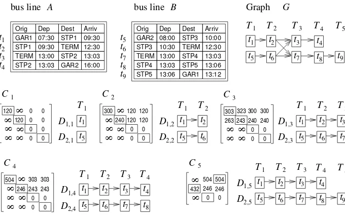
Figure 3: On the top, 2 tables of 2 bus lines containing 9 tasks, and the graph generated by those tables; On the next two rows it is shown a cost matrix Cm built in iterationmfollowed by the set of the partial duties constructed according with the solution of the Assignment Problem for that matrix.
Algorithm 1: ConstructSolution(G)
/* receive a multipartite graph G as defined */
1 begin
2 Set all dutiesDi,0=∅fori= 1,2, ..., d;
3 form←1 to kdo
4 Take the layerTmfrom G;
5 Set up the cost matrix Caccording to functionf;
6 Solve the assignment problem described by cost matrixC;
7 Assigning the tasks fromTmto each partial dutyDi,ml −1,
i= 1,· · ·, d according to assignment solution;
8 Remove all empty duty fromD;
9 returnD;
[image:14.595.131.471.428.598.2]layer, it builds the matrixC1. One of the solutions (of the Assignment Problem) is marked with rectangles which setsD1,1= (t1) andD2,1= (t5) (see first pair of partial duties on the right of matrixC1). In the second iteration (m= 2) it finds that T2 = {t2, t6}. For this layer, it builds the matrix C2, again, the solution is marked with rectangles which sets D1,2= (t1, t2) and D2,2 = (t5, t6) (shown in the right of matrix C2). The same applies to iteration 3 and 4. At the last iteration (m= 5) it finds thatT5={t9}. For this layer, it builds the last matrix
C5 where the solution is marked with rectangles and sets D1,5 = (t1, t2, t3, t4) andD2,5= (t5, t6, t7, t8, t9). Note that it assigned dummy tasks to dutyD1,5 in this last step. Since all tasks are set into layers, the algorithm ends. Thus, we setD1←D1,5andD2←D2,5.
3.4 Improvement Phase
A duty cut m on a dutyDi, denoted by CDmi, is a partition of the tasks of Di
into two sets of tasks forming two partial duties:left partial dutyDl
i,m andright
partial dutyDri,m+1,m= 1,· · · , k−1. A cut m on the set D, denoted by Cm
D, is a set of duty cut m, i.e. is the
set of the partial duties formed by the duty cuts on all duties on Dsuch that D=Dl
m∪ Dmr+1 whereDml ={Di,ml , i= 1,· · · ,|D|}andDrm+1={Di,mr +1, i= 1,· · · ,|D|}.
Lemma 1. IfCm
D is cutmon the setDthen duties fromDml may be recombined
with Dr
m+1 forming a new set of dutiesD in such a way that f(D)≥f(D).
Proof. LetDbe an instance of the set of duties constructed by algorithm 1. Let
CDm be a cut m on D (1 ≤ m ≤ k−1). Let E be a square matrix |D| × |D| where each line i(i= 1,2, ...,|D|) corresponds to the partial duty Dl
i,m ∈ Dlm, each columnj (j= 1,2, ...,|D|) corresponds to the partial dutyDr
j,m+1∈ Drm+1 and each entry ei,j corresponds to the cost of assigning all tasks of the partial dutyDr
j,m+1at the end of the partial dutyDli,m, i.e.ei,j=f(Dli,m, Drj,m+1) (the functionf used here is the same used in the construction phase) is element of the cost matrix E used by assignment problem. Since, the set of duties Dbelongs to the matrix E (it is the diagonal ei,i for i= 1,2, ...,|D|) and the solution of the assignment problem that recombinesDlmwithDmr+1into a new set of duties D, then f(D)≥f(D), the assertion follows from the minimum solution found
by the assignment problem.
Let Recombine(Cm
D) be an operation which receives cut m on the set D,
1≤m≤k−1, and recombine the partial duties as stated by Algorithm 2. LetD be the set of duties obtained by performing a Recombineoperation on the set of dutiesD. It follows from Lemma 1 thatf(D)≥f(D). However, if
Algorithm 2: Recombine(Cm
D)
1 begin
2 Recombine the partial dutiesDlmandDrm+1 ofDinto a new set of dutiesD according to the assignment problem solution using the cost matrixE as defined in the proof of Lemma 1;
3 Remove all empty duty fromD;
4 returnD;
otherwise (f(D) =f(D)) and both sets are equivalent. In any case, setD ← D at the end of each iteration.
The general improvement algorithm (Algorithm 5) uses two algorithms:Imp1 and Imp2. Algorithm Imp1 (Algorithm 3) performs successive cuts m on the set Dand tries to recombine them. AlgorithmImp2 (Algorithm 4) scans tasks with overtime and tries to reassign them to other duties in order to reduce the total cost.
Algorithm 3: Imp1(D)
1 begin
2 form←1 to k−1 do
3 D ←Recombine(Cm
D);
4 Remove all empty duty fromD;
5 returnD;
Letlot(Di) be the index of the last no dummy task of dutyDiifot(Di)>0 (it has overtime), otherwiselot(Di) = 0, i.e.lot(Di) = maxku=1{u|(ti,u∈Di∧(ti,u) is not dummy task ∧(ot(Di)>0),0}.
Algorithm 4: Imp2(D)
1 begin
2 fori←1 to |D|do
3 m←lot(Di)−1 ;
4 if m >0 then
5 D ←Recombine(Cm
D);
6 Remove all empty duty fromD;
7 returnD;
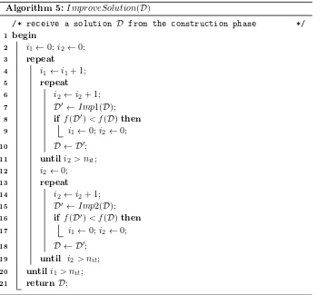
solution in a next iteration. Thus, the general improvement algorithm is stated by Algorithm 5. The algorithm ends after performing the two proceduresImp1 andImp2 without improvement for nittimes.
Algorithm 5: ImproveSolution(D)
/* receive a solution D from the construction phase */
1 begin
2 i1←0;i2←0;
3 repeat
4 i1←i1+ 1;
5 repeat
6 i2←i2+ 1;
7 D ←Imp1(D);
8 if f(D)< f(D)then
9 i1←0;i2←0;
10 D ← D;
11 untili2> nit;
12 i2←0;
13 repeat
14 i2←i2+ 1;
15 D ←Imp2(D);
16 if f(D)< f(D)then
17 i1←0;i2←0;
18 D ← D;
19 until i2> nit;
20 untili1> nit;
[image:17.595.131.491.171.496.2]21 returnD;
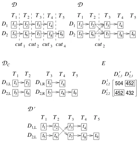
Figure 4 shows a sample of an iteration performed by algorithmImp1. The initial bus lines, graph and duties built by algorithm 1 are the same shown in Figure 3. The cost of the initial solutionDisf1(D1)+f1(D2) = 504+432 = 936. There are 5 layers in the graph. Thus, there are 4 possible cuts: cut1 between layersT1 andT2,cut2 between layersT2 andT3, cut3 between layersT3 andT4 and cut4 between layers T4 and T5. In this figure it is considered thecut2 (see Figure 4 top right). This cut will generate theCD2 ={{Dl
1,2, Dl2,2},{Dr1,3, Dr2,3}} where Dl
T5 t9 1,L 2,L D D 1 2 D D 1 2 D D D D 1,L 2,L 1,R 2,R D D 3 7 T3 t
t t8 t4 T4 T5
t9
D
cut cut cut cut t1 t5 T1 t t T2 2 6
1 2 3 4
3
7
T3
t
t t8 t4 T4 t1 t5 T1 t t T2 2 6 3 7 T3 t
t t8
t4 T4 T5
t9 t1 t5 T1 t t T2 2 6 504 452 432 452
D
cut t1 t5 T1 t t T2 2 6 3 7 T3 tt t8 t4 T4 T5
2
t9
D
C E [image:18.595.186.419.107.347.2]D’
1,3 D D 2,2 D D 1,2 l 2,3 r l rFigure 4:A sample of an iteration with a cut between layersT2andT3.
is the cost of 480 minutes of work time plus 50% of 48 minutes of overtime;
e1,2 = f(D1l,2, D2r,3) = 452 which is the cost of 312 minutes of work plus 120 minutes of idle time and 20 minutes as a penalization for bus line change;e2,1=
f(Dl
2,2, D1,3r) = 432 which is the cost of 420 minutes of work plus 12 minutes of idle time and 20 minutes as a penalization for bus line change. The solution of the Assignment Problem is shown in rectangles which is the set {e1,2, e2,1}. Thus, D ={D1, D2} where D1 = (t1, t2, t7, t8, t9) and D2= (t5, t6, t3, t4). The cost of the solutionD isf(D) = 904 which is smaller than the costf(D) = 936. Thus, theD is an improvement overD. Naturally, if the penalization for a bus line change were too high (above 36 minutes), this improvement should not be possible. Note that, procedure Imp2 may only perform cut3 which cut the last non dummy taskt4of dutyD1which has overtime. Therefore, in this particular case, procedureImp2 does not improve the solution.
4
Computational Complexity Analysis
Anywayd,sm e|D| depend on the task numbernt, that isk < maxs |D| dnt, wheremaxs=max{sm, m= 1, . . . , k}. An assignment problem is solved k times for each iteration ofImp1. The Imp2 is only applied for the last layer where there is overtime. Thus, the time complexity ofImp1andImp2is O(nt4). Usually these proceduresImp1 and Imp2 are not applied more than nt times. Therefore, we conclude that the overall complexity of our algorithm is O(nt5).
5
Computational Results and Analysis
Algorithm GraphBDSP is tested using real-world instances4from a large Brazil-ian metropolitan transportation company obtained of different days in a year. The instances are listed below; being the numerical part of the name an indi-cation of the number of tasks (e.g. CV412 contains 412 tasks): CV412, CC130, CC251, CC512, CC761, CC1000, CC1253, CC1517, CC2010 and C2313. The last three instances (CC1517, CC2010, C2313) are real cases, while the remaining were randomly created by extracting of vehicle blocks from these real instances. Our algorithm was coded in Pascal language. All these computational tests were carried out on a PC with an Intel 2.8Ghz processor and 8GB of RAM memory, running Windows operational system.
For the solution of the assignment problem we used the algorithm proposed by [Carpaneto and Toth, 1987], which combines the Hungarian method and the Shortest Augmenting Path method. To get the solution of the integer linear pro-gramming (ILP) the CBC solver [Ralphs, 2015] were used. CBC is maintained by IBM researchers, which is pretty competitive to current state-of-the-art com-mercial ILP solvers.
5.1 Computational Results
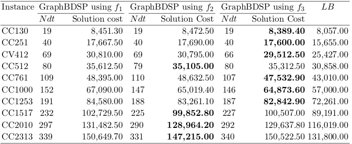
Table 3 lists the results obtained by our GraphBDSP using the functions f1,
f2 and f3 by the construction of the initial solution. We set up the parameters
pblg = 1 (penalty for each bus line change) andnit = 4 (number of iterations without solution improvement). For each instance, the number of duties (N dt) in the solution, the solution cost in minutes paid are shown. The best solution cost for each instance is highlighted in bold. The LB column shows the value of lower bound for the BDSP computed according to the mathematical model (ILP model) for personnel scheduling into a fixed place (named MPF), following the model proposed by [Bodin et al., 1983]. In this model, information on the spatial availability of the driver is ignored, thus a solution reached by this model is not a feasible BDSP solution.
Table 3:Results obtained by the proposed algorithm compared withLB
Instance GraphBDSP usingf1 GraphBDSP usingf2 GraphBDSP usingf3 LB
N dt Solution cost N dt Solution Cost N dt Solution Cost
CC130 19 8,451.30 19 8,472.50 19 8,389.40 8,057.00
CC251 40 17,667.50 40 17,690.00 40 17,600.00 15,655.00
CV412 69 30,810.00 69 30,795.00 66 29,512.50 25,427.00
CC512 80 35,612.50 79 35,105.00 80 35,312.50 30,858.00
CC761 109 48,395.00 110 48,632.50 107 47,532.90 43,010.00
CC1000 152 67,090.00 147 65,019.40 146 64,873.60 57,000.00
CC1253 191 84,580.00 188 83,261.10 187 82,842.90 72,261.00
CC1517 232 102,729.50 225 99,852.80 227 100,507.00 89,191.00
CC2010 297 131,482.50 290 128,964.20 292 129,637.80 116,019.00
CC2313 339 150,649.70 331 147,215.00 340 150,522.50 131,800.00
Running time was short, being 4min:4s the longest for instance CC2313 using function f1. The best results were obtained using functionsf2 andf3.
5.2 Improvement Procedures Analysis
[image:20.595.127.477.491.571.2]Table 4 indicates how much the initial solution cost can be reduced by using each procedure Imp1 andImp2 (alone and combined) in all cases using functionf3. Columns Red% mean the percentage of reduction in relation to initial solution cost.
Table 4:Comparison between improvement procedures
Instance Initial Sol. Experiment 1 Experiment 2 Experiment 3
Imp1 Red% Imp2 Red% Imp1 +Imp2 Red%
CV412 33,394.80 29,512.50 11.63 30,897.30 7.48 29,512.50 11.63
CC1000 74,637.00 65,442.00 12.32 68,550.50 8.15 64,873.60 13.08
CC1253 95,622.00 82,955.40 13.25 88,486.90 7.46 82,842.90 13.36
CC2313 172,660.40 150,635.00 12.76 158,088.00 8.44 150,522.50 12.82
The highest gain by using bothImp1andImp2was for instance CC1000, which obtained an additional reduction of 0.88% in relation to the reduction obtained by using only Imp1. Although such a gain was small in percentage, it is worth noting that its economic value can be rather significant.
5.3 Results with the Set Covering Problem - SCP
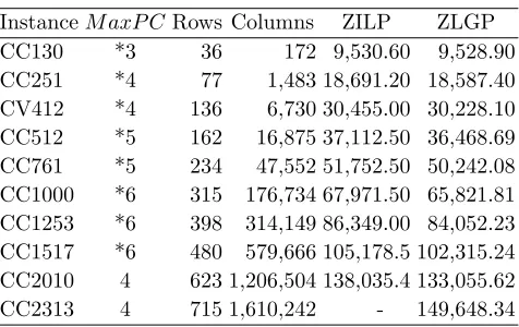
[image:21.595.184.422.460.610.2]This section presents results for the BDSP modeled as a SCP. For small instances, the optimal value could be obtained by using ILP solver, whereas for large in-stances, lower bounds was computed using the subgradient method to solve a La-grangian relaxation problem for SCP according to [Beasley, 1987, Umetani and Yagiura, 2007]. As mentioned at the beginning of this paper, the total number of possible columns in a SCP instance is usually very high, mainly for the largest BDSP instances. Thus, we used a classical heuristic technique to reduce (gener-ate) the number of columns based on a maximum number of PWOs per column (M axP C), limiting the minimum and maximum duration for each PWOs of 60 and 100 minutes, respectively. A similar procedure was also used by [De Leone et al., 2011a]. In this paper the values of M axP C were estimated taking into account some previous real scheduling provided by the transportation company. Table 5 presents results obtained from BDSP solution using the SCP model. An asterisk (*) before the number indicates that all possible columns have been gen-erated. Values without the asterisk indicate that the instance could have more columns with more M axP C PWOs, but they were not generated in order to keep the problem in a solvable size.
Table 5:Results obtained with SCP model
InstanceM axP CRows Columns ZILP ZLGP
CC130 *3 36 172 9,530.60 9,528.90
CC251 *4 77 1,483 18,691.20 18,587.40
CV412 *4 136 6,730 30,455.00 30,228.10
CC512 *5 162 16,875 37,112.50 36,468.69
CC761 *5 234 47,552 51,752.50 50,242.08
CC1000 *6 315 176,734 67,971.50 65,821.81
CC1253 *6 398 314,149 86,349.00 84,052.23
CC1517 *6 480 579,666 105,178.5 102,315.24
CC2010 4 623 1,206,504 138,035.4 133,055.62
CC2313 4 715 1,610,242 - 149,648.34
solving of ILP, ZLGP is the Lagrangian lower bound [Beasley, 1987, Umetani and Yagiura, 2007]. To obtain ZILP a running time limit of 24 hours was adopted. Table 5 shows it was possible to obtain the ZILP value for nearly all the instances, except for instance CC2313 due to the high number of columns and the high running time without obtaining the solution (more than 24 hours waiting).
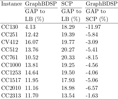
5.4 Comparison of Results
Table 6 shows relative percentage deviation, named GAP. First column is the GAP from the best solution cost from GraphBDSP (Table 3) in relation to LB. Second column is the GAP from the best solution cost from SCP (ZILP or ZLGP value) (Table 5) in relation to LB (Table 3). Third column is the GAP from the best solution cost from GraphBDSP (Table 3) in relation to the best solution cost from SCP (Table 5).
Note that the GraphBDSP GAP to LB are apparently high due to LB
[image:22.595.200.403.403.575.2]quality, since the MPF formulation is a fairly relaxed model to BDSP [Bodin et al., 1983], but it is the best known model to get lower bound for BSDP. The GraphBDSP solution costs were kept above the lower bound (LB) by between 4.13% and 16.07%.
Table 6:Comparison GraphBDSP results against LB and SCP results
Instance GraphBDSP SCP GraphBDSP
GAP to GAP to GAP to
LB (%) LB (%) SCP (%)
CC130 4.13 18.29 -11.97
CC251 12.42 19.39 -5.84
CV412 16.07 19.77 -3.09
CC512 13.76 20.27 -5.41
CC761 10.52 20.33 -8.15
CC1000 13.81 19.25 -4.56
CC1253 14.64 19.50 -4.06
CC1517 11.95 17.93 -5.06
CC2010 11.16 18.98 -6.57
CC2313 11.70 13.54 -1.63
means optimum solution for the BDSP, even for the Lagrangian lower bound for these instances. Note that, we got the optimum solution for the SCP instances (except instance CC2313).
6
Conclusions
We presented a deterministic 2-phase algorithm, named GraphBDSP, to tackle the bus driver scheduling problem based on Brazilian real instances, from an urban public transportation company. This algorithm produced competitive re-sults comparing with SCP-based approach providing good result for huge real instances with more than 2,300 tasks within reasonable computing time. To the best of our knowledge this is the largest real instance in the literature and the GraphBDSP represents a new approach applied to the bus driver scheduling problem. The results are compared against to lower bounds computed by math-ematical programming. The computational performance of the GraphBDSP was very satisfactory regarding both the solution quality and the running time.
We compared three different cost functions, which the functionf3 based on idle time and overtime presented best results for most cases instead of focusing on paid time only. Although the best solution for the large instance was achieved with the functionf2 (idle time). Anyway, the objective functionf1 focusing on paid time was not the best option.
GraphBDSP is a deterministic algorithm that uses no random operations, i.e., it always find the same solution for the same input. In addition, it has only one parameter to tune (nit), so it uses an easy parameter tuning. GraphBDSP is quite flexible to changes of rules. The adapt5ations regarding the new rules are needed to compute the cost matrix for each bipartite graph, without changing the model. Thus, we believe it is extensible to other crew scheduling problems.
Our algorithm meets the criteria defined by [Cordeau et al., 2002] for heuris-tic methods. The simplicity criterion is met because the proposed algorithm requires only one parameter to tune and uses a classical well-known assignment problem, which is easily solved by polynomial running time algorithm. The flex-ibility criterion is also observed when incorporating new rules. A reasonable accuracy and speed criteria are also observed as shown in section 5.
Acknowledgments
We would like to thank the anonymous referees for their constructive comments, which led to a clearer presentation of this paper. We would also like to thank CNPq (process 306754/2015-0), CAPES and Funda¸c˜ao Arauc´aria for their fi-nancial support.
References
[Beasley, 1987] Beasley, J. E. (1987). An algorithm for set covering problems. Euro-pean Journal of Operational Research, 31:85–93.
[Beasley and Chu, 1996] Beasley, J. E. and Chu, P. C. (1996). A genetic algorithm for the set covering problem. European Journal of Operational Research, 94(2):392–404. [Bodin et al., 1983] Bodin, L., Golden, B., Assad, A., and Ball, M. (1983). Routing and scheduling of vehicles and crews - the state of the art. Computers and Operations Research, 10(2):63–212.
[Bornd¨orfers, 2010] Bornd¨orfers, R. (2010).Aspects of Set Packing, Partitioning, and Covering. PhD thesis, Technische Universit¨at Berlin.
[Caprara et al., 1999] Caprara, A., Fischetti, M., and Toth, P. (1999). A heuristic method for the set covering problem. Operations Research, 47:730–743.
[Carpaneto and Toth, 1987] Carpaneto, G. and Toth, P. (1987). Primal-dual algror-ithms for the assignment problem. Discrete Applied Mathematics, 18(2):137 – 153. [CASPT2015, 2015] CASPT2015 (2015). Conference on Advanced Systems in Public
Transport. http://www.caspt.org.
[Constantino et al., 2014] Constantino, A. A., Landa-Silva, D., de Melo, E. L., de Mendon¸ca, C. F. X., Rizzato, D. B., and Rom˜ao, W. (2014). A heuristic algo-rithm based on multi-assignment procedures for nurse scheduling. Annals of Opera-tions Research, 218(1):165–183.
[Cordeau et al., 2002] Cordeau, J. F., Gendreau, M., Laporte, G., Potvin, J. Y., and Semet, F. (2002). A guide to vehicle routing heuristics. Journal of the Operational Research Society, 53(5):512–522.
[Daduna and Wren, 1988] Daduna, J. and Wren, A. (1988). Computer-aided Transit Scheduling: Proceedings of the Fourth International Workshop on Computer-Aided Scheduling of Public Transport. Lecture Notes in Economics and Mathematical Sys-tems. Springer-Verlag.
[D’Annibale et al., 2007] D’Annibale, G., Leone, R. D., Festa, P., and Marchitto, E. (2007). A new meta-heuristic for the bus driver scheduling problem: GRASP com-bined with rollout. In 2007 IEEE Symposium on Computational Intelligence in Scheduling, CISched 2007, Honolulu, Hawaii, USA, April 2-4, 2007, pages 192–197. [De Groot and Huisman, 2008] De Groot, S. W. and Huisman, D. (2008). Vehicle and Crew Scheduling: Solving Large Real-World Instances with an Integrated Approach, pages 43–56. Springer Berlin Heidelberg, Springer Berlin Heidelberg, Berlin, Heidel-berg.
[De Leone et al., 2011a] De Leone, R., Festa, P., and Marchitto, E. (2011a). A bus driver scheduling problem: a new mathematical model and a GRASP approximate solution. J. Heuristics, 17(4):441–466.
[De Leone et al., 2011b] De Leone, R., Festa, P., and Marchitto, E. (2011b). Solving a bus driver scheduling problem with randomized multistart heuristics. International Transactions in Operational Research, 18(6):707–727.
[Fores, 2001] Fores, S. (2001). Column generation approaches to bus driver scheduling. PhD thesis, School of Computing.
[Huisman et al., 2005] Huisman, D., Freling, R., and Wagelmans, A. P. M. (2005). Multiple-depot integrated vehicle and crew scheduling. Transportation Science, 39(4):491–502.
[Laurent and Hao, 2008] Laurent, B. and Hao, J.-K. (2008). Simultaneous vehicle and crew scheduling for extra urban transports. In Nguyen, N., Borzemski, L., Grzech, A., and Ali, M., editors,New Frontiers in Applied Artificial Intelligence, volume 5027 ofLecture Notes in Computer Science, pages 466–475. Springer Berlin Heidelberg. [Li et al., 2015] Li, H., Wang, Y., Li, S., and Li, S. (2015). A Column Generation
Based Hyper-Heuristic to the Bus Driver Scheduling Problem. Discrete Dynamics in Nature and Society, 2015:1–10.
[Li, 2005] Li, J. (2005). A self-adjusting algorithm for driver scheduling. Journal of Heuristics, 11(4):351–367.
[Li and Kwan, 2003] Li, J. and Kwan, R. S. (2003). A fuzzy genetic algorithm for driver scheduling. European Journal of Operational Research, 147(2):334 – 344. [Liping Zhao, 2006] Liping Zhao (2006). A heuristic method for analyzing driver
scheduling problem. IEEE Transactions on Systems, Man, and Cybernetics - Part A: Systems and Humans, 36(3):521–531.
[Ma et al., 2016] Ma, J., Ceder, A. A., Yang, Y., Liu, T., and Guan, W. (2016). A case study of Beijing bus crew scheduling: a variable neighborhood-based approach: VNS Algorithm for Bus Crew Scheduling. Journal of Advanced Transportation, 50(4):434– 445.
[Mauri and Lorena, 2007] Mauri, G. R. and Lorena, L. A. N. (2007). A new hybrid heuristic for driver scheduling. Int. J. Hybrid Intell. Syst., 4(1):39–47.
[Mesquita and Paias, 2008] Mesquita, M. and Paias, A. (2008). Set partitioning/covering-based approaches for the integrated vehicle and crew scheduling problem. Computers and Operations Research, 35(5):1562–1575.
[Ohlsson et al., 2001] Ohlsson, M., Peterson, C., and S¨oderberg, B. (2001). An efficient mean field approach to the set covering problem. European Journal of Operational Research, 133(3):583–595.
[Pentico, 2007] Pentico, D. W. (2007). Assignment problems: A golden anniversary survey. European Journal of Operational Research, 176(2):774–793.
[Portugal et al., 2009] Portugal, R., Loureno, H., and Paixo, J. (2009). Driver schedul-ing problem modellschedul-ing. Public Transport, 1(2):103–120.
[Ralphs, 2015] Ralphs, T. (2015 (accessed 30-May-2015)). CBC MILP. https:// projects.coin-or.org/Cbc.
[Santos and Mateus, 2007] Santos, A. G. d. and Mateus, G. R. (2007). Hybrid ap-proach to solve a crew scheduling problem: an exact column generation algorithm improved by metaheuristics. In 7th International Conference on Hybrid Intelligent Systems (HIS 2007), pages 107–112.
[Shen and Kwan, 2001] Shen, Y. and Kwan, R. S. K. (2001). Computer-Aided Schedul-ing of Public Transport, chapter Tabu Search for Driver SchedulSchedul-ing, pages 121–135. Springer Berlin Heidelberg, Berlin, Heidelberg.
[Shijun Chen, 2013] Shijun Chen, Y. S. (2013). An improved column generation al-gorithm for crew scheduling problems. Journal of Information and Computational Science, 10(1):175–183.
[Silva and Reis, 2014] Silva, G. P. and Reis, A. F. d. S. (2014). A study of different metaheuristics to solve the urban transit crew scheduling problem. Journal of Trans-port Literature, 8(4):227–251.
[Umetani and Yagiura, 2007] Umetani, S. and Yagiura, M. (2007). Relaxation heuris-tics for the set covering problem. Journal of the Operations Research Society of Japan, 50(4):350–375.
[Wren and Rousseau, 1995] Wren, A. and Rousseau, J.-M. (1995).Bus Driver Schedul-ing - An Overview, volume 430 of Lecture Notes in Economics and Mathematical Systems, pages 173–187. Springer Berlin Heidelberg.
[Wren and Wren, 1995] Wren, A. and Wren, D. O. (1995). A genetic algorithm for public transport driver scheduling. Computers and Operations Research, 22(1):101– 110.