Type Reduction Operators for Interval Type–2
Defuzzification
Thomas A. Runklera, Chao Chenb, Robert Johnc
a Siemens AG, Corporate Technology, 81730 Munich, Germany, Email:
bLaboratory for Uncertainty in Data and Decision Making (LUCID), University of
Nottingham, Wollaton Road, Nottingham, NG8 1BB, UK Email: [email protected]
cLaboratory for Uncertainty in Data and Decision Making (LUCID), University of
Nottingham, Wollaton Road, Nottingham, NG8 1BB, UK Email: [email protected]
Abstract
Fuzzy sets are an important approach to model uncertainty. Defuzzification maps fuzzy sets to non–fuzzy (crisp) values. Type–2 fuzzy sets model uncer-tainty in the degree of membership in a fuzzy set. Type–2 defuzzification maps type–2 fuzzy sets to non–fuzzy values. Type reduction maps type–2 fuzzy sets to type–1 fuzzy sets, in order to make type–2 defuzzification easier and to im-plement more efficient type–2 defuzzification algorithms.
This paper is a first step towards a theoretical foundation of the emerging field of type reduction. Five mathematical properties of type reduction are defined, and two existing type reduction methods (Nie–Tan and uncertainty weight) are examined with respect to our five properties. Furthermore, two new type reduction methods are proposed: consistent linear type reduction and consistent quadratic type reduction. All our five properties are satisfied by consistent quadratic type reduction.
Keywords: defuzzification, type–2 fuzzy sets
This manuscript is the authors’ original work and has not been published nor has it
been submitted simultaneously elsewhere. All authors have checked the manuscript and have
1. Introduction
Fuzzy sets [29] are an important approach to model and process uncertain information. Fuzzy information processing (for example in fuzzy rule based systems [14, 26]) usually yield fuzzy sets as outputs. If non–fuzzy outputs are needed (for example in control applications [7, 18]), these can be obtained from fuzzy outputs using defuzzification. Many defuzzification methods have been proposed during the last decades, for an overview see [19, 20, 25], and the mathematical properties of defuzzification have been studied in [24].
Interval type–2 fuzzy sets [13, 15, 30] are extensions of (type–1) fuzzy sets, where the degrees of membership in a fuzzy set may be uncertain. Interval type–2 fuzzy information processing yields interval type–2 fuzzy sets as outputs, which can be converted to non–fuzzy outputs using interval type–2 defuzzifica-tion. One of the most popular methods for interval type–2 defuzzification is the Karnik–Mendel algorithm [11]. The mathematical properties of interval type–2 defuzzification have been studied in [22].
Recently, alternative methods for interval type–2 defuzzification have been proposed that are based ontype reduction. Type reduction of an interval type–2 fuzzy set means a mapping to a type–1 fuzzy set which then can be defuzzified using type–1 defuzzification techniques. Examples are the Nie–Tan (NT) [17] and the uncertainty weight (UW) method [23]. The relation between type– 1 defuzzification, type–2 defuzzification, and type reduction is illustrated in Fig. 1.
type–2 fuzzy set
type–1 fuzzy set
non–fuzzy value
-type–2 defuzzification
-type reduction type–1 defuzzification 6
The NT and UW methods (and also the CQTR and CLTR methods proposed in this paper) are different from the Karnik–Mendel approach.These methods reduce each interval type–2 fuzzy set to a type–1 fuzzy set upfront, and then perform ordinary type–1 defuzzification. These methods can therefore also be viewed as a tool to design type–1 membership functions in scenarios with dif-ferent levels of uncertainty for difdif-ferent decision options.
Type–reduction based interval type–2 defuzzification reduces interval type– 2 fuzzy sets to type–1 fuzzy sets upfront, so we lose some ability to explicitly consider the specific uncertainty of the memberships which is considered an important advantage of interval type–2 fuzzy sets over type–1 fuzzy sets. It was shown however for typical fuzzy controller scenarios that the NT method and its variants yield very good approximations of the Karnik–Mendel algorithm at a reduced computational cost [12, 23], which appears beneficial for a large number of real–world applications.
The emerging field of type reduction needs a theoretical foundation that en-ables researchers to assess, compare, and develop novel type reduction methods. So the focus of this paper is not just proposing new type reduction formulas. We also propose the required properties (a standard) for designing type reduction methods. As a first step in this direction, this paper defines five mathemat-ical properties of type reduction. There are infinitely many choices for type reduction functions. An important criterion for type reduction functions is (mathematical and computational) simplicity, so we will focus on linear and quadratic functions in this paper. We will derive specific linear and quadratic functions to meet our five proposed properties, which will lead us to propose two new type reduction methods,consistent linear type reduction (CLTR)and consistent quadratic type reduction (CQTR).
6 and 7). Finally, we summarize the properties of all considered methods, give some illustrative examples (Section 8), and present our conclusions and ideas for future research (Section 9).
2. Type–1 and Type–2 Defuzzification
A type–1 fuzzy set [29] over a universe X is specified by a membership function u : X → [0,1], so u(x) quantifies the degree of membership of any
x∈X in the type–1 fuzzy set. Type–1 defuzzification is a functiondthat maps any type–1 fuzzy membership function to one representative crisp (non–fuzzy) value inX.
d(u(x))∈X (1)
One of the most popular type–1 defuzzification methods is thecentroiddefined as
dC(u(x)) =
R
X
u(x)·x dx R
X
u(x)dx (2)
which represents the (horizontal) position of the center of gravity (first moment) of the area between the membership function and thexcoordinate (abscissa). Many other methods for type–1 defuzzification have been proposed in the liter-ature. For an overview see [19, 20, 25].
An interval–fuzzy set [3, 9, 10] or closed interval type–2 fuzzy set [16] is specified by two membership functions: a lower membership functionu:X →
[0,1] and an upper membership functionu:X→[0,1], where
u(x)≤u(x) (3)
for allx∈X. Interval type–2 fuzzy sets can be used to model uncertainty about a membership function or to model risk in decision processes [21].
A popular interval type–2 defuzzification method is theKarnik–Mendel (KM) algorithm [11] that considers all (type–1) membership functionsu(x) between the lower and upper membership functionsu(x) andu(x), respectively,
For one dimensional universes X ⊆ R, KM computes the lower and upper
centroids that can be written as
dC(u(x), u(x)) = inf
u(x)≤u(x)≤u(x)dC(u(x)) (5)
dC(u(x), u(x)) = sup u(x)≤u(x)≤u(x)
dC(u(x)) (6)
and returns the average of these
dKM(u(x), u(x)) =
dC(u(x), u(x)) +dC(u(x), u(x))
2 (7)
The Karnik–Mendel algorithm is iterative and computationally intensive, so several enhanced methods and efficient implementations have been proposed in the literature [6, 27, 28].
Nie and Tan [17] have introduced an alternative way to interval type–2 de-fuzzification. The idea is to transform the lower and upper membership func-tionsu(x) andu(x) to one single (type–1) membership functionu(x), and then apply type–1 defuzzification, for example the centroid method, to u(x). The conversion of the lower and upper interval type–2 membership functions to one single type–1 membership function is calledtype reduction. Type reduction for interval type–2 membership functions can be viewed as an application of a two– dimensional fusion function [1, 4]. In their original paper, Nie and Tan [17] proposed theNie–Tan (NT)type reduction formula
uNT(x) = u(x) +u(x)
2 (8)
which converts an interval type–2 fuzzy set to a type–1 fuzzy set by taking the average of each respective upper and lower membership grades.
Recently, Runkleret al. [23] presented an alternative type reduction formula called theuncertainty weight (UW)method
uUW(x) = 1
2(u(x) +u(x))·(1 +u(x)−u(x))
α (9)
respective upper and lower membership grades (which is used in the Nie–Tan method), the uncertainty weight method multiplies this average by the weight factor (1 +u(x)−u(x))α, which is zero for maximum uncertainty (u(x) = 0,
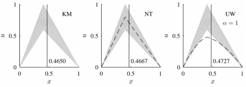
u(x) = 1) and one for minimum uncertainty (u(x) =u(x)), and which increases linearly with the uncertainty for α = 1, less than linearly for all α < 1 and more than linearly for all α >1. The experiments in [12, 23] indicated that both NT and UW can be used to yield good approximations of KM with low computational effort. Fig. 2 shows the defuzzification results of the KM, NT, and UW (α= 1) methods for an example of a triangular interval type–2 fuzzy set. The vertical solid lines indicate the defuzzification results for the three methods: dKM = 0.4650, dNT = 0.4667, and dUW = 0.4727, which are all very similar for this example. The dashed curves at the NT and UW graphs are the results of type reduction. The KM graph does not show any dashed curve because KM directly produces a non–fuzzy value from a type–2 fuzzy set, without type reduction to a type–1 fuzzy set. NT type reduction yields a (type–1) membership function that passes right through the middle of the grey area limited by the upper and lower interval type–2 membership functions. In this example, UW type reduction yields a membership function partially lying outside the grey area. The observation of this behavior was one of the main motivations to define the properties of type reduction (most specifically the so–called type–2 consistency property) which are introduced in the following section.
3. Properties of Type Reduction
0 0.5 1 x
0 0.5 1
u
0.4650 KM
0 0.5 1
x 0
0.5 1
u
0.4667 NT
0 0.5 1
x 0
0.5 1
u
0.4727 UW
α= 1
Figure 2: Defuzzification of a triangular interval type–2 fuzzy set using the KM, NT, and UW
(α= 1) methods.
purpose of these properties is to evaluate, compare, and develop type reduction methods.
Here, we only consider pointwise type reduction methods, i.e. for the com-putation of a type–1 membership degreeu(x) we only consider the lower and upper interval type–2 membership degreesu(x) and u(x) at the same pointx, but not the membership degreeu(y) andu(y) at any other pointy6=x. There-fore, we can omit the argumentxand simply write each type reduction method as a functionf : [0,1]2→[0,1] with
u=f(u, u) (10)
3.1. Type–1 Consistency
If the lower and upper interval type–2 memberships are equal, then we obtain the special case of type–1 memberships.
u=u (11)
In this case there no uncertainty about the membership, and we expect the type reduction to yield
⇒ u=u=u (12)
This means that if the uncertainty disappears, the interval type–2 fuzzy model will reduce to a conventional type–1 fuzzy model. This property corresponds to the (only) requirement that was used to derive the popular Karnik–Mendel method. It also corresponds to the notion of idempotency, which is very well known in algebra and in the field of aggregation functions [2].
Definition 1. A type reduction functionf istype–1 consistentif and only if
f(u, u) =ufor allu∈[0,1] (13)
3.2. Type–2 Consistency
Let us assume arbitrary lower and upper interval type–2 membershipsu, u∈
[0,1] with
u≤u (14)
A common interpretation of this situation is that there is uncertainty about the membership, and the membership is at leastuand at mostu.
u≤u≤u (15)
Definition 2. A type reduction functionf istype–2 consistentif and only if
u≤f(u, u)≤ufor allu, u∈[0,1] withu≤u (16)
Theorem 1. If a function is type–2 consistent, then it is type–1 consistent.
Proof. Trivial.
Type–2 consistency is related to the notion of an averaging function (a func-tion which is between the minimum and the maximum), but it is not the same because we are not assuming symmetry here. Type reduction is also closely related to the idea of ignorance functions and entropy for interval–valued fuzzy sets [5]. We are planning to investigate in a future project if adding a symmetry constraint could yield a generalized definition of type reduction in the context of averaging functions, and we want to have a closer look at the relation between type reduction and ignorance functions.
3.3. (Strict) Uncertainty Conformity
Let us assume that the membership is aroundu∗∈[0,1] with an uncertainty of±∆u, where
u∗−∆u≥0, u∗+ ∆u≤1 (17)
so we obtain
u=u∗−∆u, u=u∗+ ∆u (18)
For ∆u= 0 we have the type–1 case, and for any type–1 consistent functionf
we obtain
u=f(u∗, u∗) =u∗ (19)
type reduction operator has this property, then for two options with the same average membership but with different levels of uncertainty (spread between the lower and upper type–2 memberships) the option with lower uncertainty will be preferred over the option with higher uncertainty, so the degree of uncertainty is reflected in the type reduction process.
Definition 3. A type reduction functionf is uncertainty conformif and only if for anyu∗∈[0,1] and any ∆u1,∆u2≥0, ∆u1<∆u2with
u∗−∆u2≥0, u∗+ ∆u2≤1 (20)
the following condition holds:
f(u∗−∆u1, u∗+ ∆u1)≥f(u∗−∆u2, u∗+ ∆u2) (21)
Definition 4. A type reduction function f is strictly uncertainty conform if and only if for anyu∗∈[0,1] and any ∆u1,∆u2≥0, ∆u1<∆u2 with
u∗−∆u2≥0, u∗+ ∆u2≤1 (22)
the following condition holds:
f(u∗−∆u1, u∗+ ∆u1)> f(u∗−∆u2, u∗+ ∆u2) (23)
Lemma 1. The preconditions of Definitions 3 and 4 imply ∆u≤0.5. Proof.
Foru∗∈[0,0.5] : u∗−∆u≥0 ⇒ ∆u≤u∗≤0.5 (24) Foru∗∈[0.5,1] : u∗+ ∆u≤1 ⇒ ∆u≤1−u∗≤0.5 (25)
So foru∗∈[0,1] we have ∆u≤0.5.
Theorem 2. If a function is strictly uncertainty conform, then it is uncertainty
conform.
3.4. Ignorance of Indifference
The most uncertain interval type–2 membership values are
u= 0, u= 1 (26)
In this case we have no information about the membership at all, so we may want to completely ignore such indifferent objects
⇒ u= 0 (27)
If a type reduction operator has this property, then options with complete un-certainty will receive zero memberships and hence will receive weight zero in the defuzzification process.
Definition 5. A type reduction functionf ignores indifference if and only if
f(0,1) = 0 (28)
4. Properties of the Nie–Tan Method
The Nie–Tan (NT) method [17] is specified by the type reduction function
fNT(u, u) =
u+u
2 (29)
In this section we examinefNTwith respect to the five properties defined in the previous section. The properties of the NT and all other methods considered in this paper will be summarized in section 8.
Theorem 3. The Nie–Tan type reduction function is type–1 consistent.
Proof.
fNT(u, u) =u+u
2 =ufor allu∈[0,1] (30)
Theorem 4. The Nie–Tan type reduction function is type–2 consistent.
Proof. For allu, u∈[0,1] withu≤u fNT(u, u) =u+u
2 ≥
u+u
2 =u (31)
fNT(u, u) =
u+u
2 ≤
u+u
Theorem 5. The Nie–Tan type reduction function is uncertainty conform.
Proof. For any u∗∈[0,1] and any ∆u≥0 we obtain
fNT(u∗−∆u, u∗+ ∆u) =u
∗−∆u+u∗+ ∆u
2 =u
∗ (33)
so for ∆u1≥∆u2
fNT(u∗−∆u1, u∗+ ∆u1) = fNT(u∗−∆u2, u∗+ ∆u2) = u∗(34)
⇒ fNT(u∗−∆u1, u∗+ ∆u1) ≥ fNT(u∗−∆u2, u∗+ ∆u2) (35)
Theorem 6. The Nie–Tan type reduction function is not strictly uncertainty
conform.
Proof. From (34) follows
fNT(u∗−∆u1, u∗+ ∆u1) > f6 NT(u∗−∆u2, u∗+ ∆u2) (36)
Theorem 7. The Nie–Tan type reduction function does not ignore indifference.
Proof.
fNT(0,1) = 0 + 1
2 = 0.56= 0 (37)
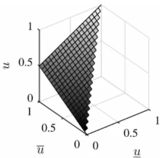
Fig. 3 shows the graph of the NT function over the triangle (u, u)∈[0,1]2with
u≤u. The graph of the NT function is a triangle with the edge points (u, u, u) = (0,0,0), (1,1,1), and (0,1,0.5), which contradicts ignorance of indifference. The graph of the NT function is linear with a slope of 0.5 along both the uand u
axes.
5. Properties of the Uncertainty Weight Method
Runkleret al. proposed the uncertainty weight (UW) method [23] specified by the type reduction function
fUW(u, u) = 1
2(u+u)·(1 +u−u)
α (38)
with the parameterα >0. Obviously, UW converges to NT asαapproaches 0.
0 1 0.5
1
u
u
0.5 1
u
0.5 0 0
Figure 3: Graph of the NT function.
In this section we examine fUW with respect to the five properties defined in this paper.
Theorem 8. The uncertainty weight type reduction function is type–1
consis-tent.
Proof.
fUW(u, u) = 1
2(u+u)·(1 +u−u)
α=ufor allu
∈[0,1] (40)
Theorem 9. The uncertainty weight type reduction function is not generally
(i.e. for anyα >0) type–2 consistent. Proof. Let for example u= 0.5,u= 1. Then
fUW(0.5,1) = 1
2(0.5 + 1)·(1 + 0.5−1)
α= 0.5 3
2α+1 6≥0.5 =u for 2α+1>3 ⇒ α > log 3
log 2−1≈0.585 (41)
Theorem 10. The uncertainty weight type reduction function is strictly
uncer-tainty conform.
Proof.
fUW(u∗−∆u, u∗+ ∆u) = 1
2(u
∗−∆u+u∗+ ∆u)·(1 +u∗−∆u−u∗−∆u)α=u∗(1−2∆u)α (42) is strictly monotocially decreasing with ∆u for ∆u ≤0.5 (Lemma 1) and for
Theorem 11. The uncertainty weight type reduction function is uncertainty
conform.
Proof. Follows from Theorems 2 and 10.
Theorem 12. The uncertainty weight type reduction function ignores
indiffer-ence.
Proof.
fUW(0,1) = 1
2(0 + 1)·(1 + 0−1)
α= 0 (43)
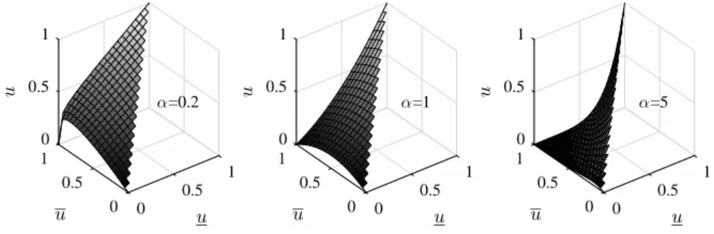
Fig. 4 shows the graphs of the UW function forα∈ {0.2,1,5}. All three graphs are nonlinear but smooth, and contain the points (u, u, u) = (0,0,0), (1,1,1), and (0,1,0), corresponding to ignorance of indifference. Forα= 0.2 (left), the UW function looks very similar to the NT function at Fig. 3, only the very edge at u= 0 and u= 1 is bent fromu= 0.5 to u= 0 (ignorance of indifference). Depending on the value of the parameter αthe graph of the UW function is bent in different ways. It is monotonically increasing along the u axis with increasing (α = 0.2) or decreasing slope (α = 5). It is however not generally monotonic along theuaxis. Consider for example the front edge curve atu= 0 which is distinctly bent up for medium values of u ≈ 0.5 for α = 0.2 (left) and α = 1 (center). For α = 5 (right), the UW function always yields very small memberships u ≈ 0 except near the main diagonal at u = u, where it yieldsu=u=u(type–1 consistency). Forα= 1 (center), the UW function is quite flat along theuaxis, and almost linearly increases along theuaxis, so it approximates the functionu=u.
6. Linear Type Reduction
Besides NT and UW we can construct infinitely many type reduction func-tionsf. For reasons of simplicity we first consider linear functions and derive specific instances of linear functions trying to satisfy our five proposed proper-ties. So we start with the general case of linear functions for type reduction
0 1 0.5 1 u u α=0.2 0.5 1 u 0.5 0 0 0 1 0.5 1 u u α=1 0.5 1 u 0.5 0 0 0 1 0.5 1 u u α=5 0.5 1 u 0.5 0 0
Figure 4: Graphs of the UW function forα∈ {0.2,1,5}.
with arbitrary parametersa, b, c∈R. If we require type–1 consistency, then we
obtain
u= 0, u= 0, u= 0 ⇒ c= 0 (45)
u= 1, u= 1, u= 1 ⇒ 1 =a+b+c ⇒b= 1−a (46)
and so
u=a·u+ (1−a)·u (47)
If we further require type–2 consistency, then we obtain
u≤a·u+ (1−a)·u ⇒ (1−a)·(u−u)≥0 ⇒ a≤1 (48)
a·u+ (1−a)·u≤u ⇒ a·(u−u)≥0 ⇒ a≥0 (49)
which leads us to
Definition 6. Theconsistent linear type reduction (CLTR)function is defined as
fCLTR(u, u) =a·u+ (1−a)·u (50) witha∈[0,1]
for the upper membership grades. Fora= 0, CLTR will yield the upper mem-bership function; for a = 0.5, CLTR will yield the average of the upper and lower membership functions, which is also the result of the NT type reduction function (so the NT type reduction function is a special case of the CLTR func-tion); and for a= 1, CLTR will yield the lower membership function. For all other values ofa∈[0,1], CLTR will linearly interpolate between these special cases.
Theorem 13. The consistent linear type reduction function is type–1 and type–
2 consistent.
Proof. Follows immediately from the requirements for consistent linear type reduction functions (45)–(49).
Theorem 14. The consistent linear type reduction function is uncertainty
con-form if and only ifa≥0.5. Proof.
fCLTR(u∗−∆u, u∗+ ∆u)
=a·(u∗−∆u) + (1−a)·(u∗+ ∆u) =u∗+ (1−2a)·∆u (51) is monotocially decreasing with ∆uforα∈[0.5,1].
Theorem 15. The consistent linear type reduction function is strictly
uncer-tainty conform if and only ifa >0.5.
Proof. (51) is strictly monotocially decreasing with ∆uforα <(0.5,1].
Notice that the NT type reduction function is the only instance of the CLTR function that is uncertainty conform but not strictly uncertainty conform.
Theorem 16. The consistent linear type reduction function ignores indifference
if and only ifa= 1. Proof.
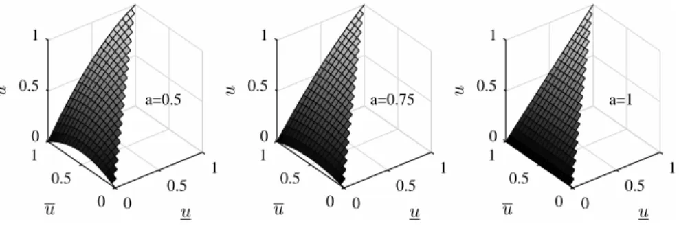
Fig. 5 shows the graphs of the CLTR function fora∈ {0.5,0.75,1}. All three graphs are triangles through (u, u, u) = (0,0,0) and (1,1,1). The third edge of each triangle is at (0,1,1−a). The intersection of all CLTR graphs is the unit main diagonal through (0,0,0) and (1,1,1) (type–1 consistency). All three graphs are linear with non–negative slopes along u and u. The slope is zero along u for a = 1. All these three CLTR instances are uncertainty conform, because a∈[0.5,1]. The left graph (a = 0.5) corresponds to the NT function at Fig. 3. The right graph (a= 1) corresponds to the only CLTR function that ignores indifference, u=u, which is approximately equal to the UW function forα= 1 (Fig. 4 center). For a= 1, the CLTR function always yieldsu=u, so the complete information aboutuis lost in this case. Hence, if we want to keep the information about bothuand u, and at the same type satisfy all our five properties, then we have to use a nonlinear type reduction function.
0 1 0.5 1 u u a=0.5 0.5 1 u 0.5 0 0 0 1 0.5 1 u u a=0.75 0.5 1 u 0.5 0 0 0 1 0.5 1 u u a=1 0.5 1 u 0.5 0 0
Figure 5: Graphs of the CLTR function fora∈ {0.5,0.75,1}.
7. Nonlinear Type Reduction
should be able to satisfy all five proposed properties.
To find such a function we start with the linear approach (44) and add a nonlinear term. This nonlinear term should be suitable to indicate indifference, so it should containuandu. In order to stay type–1 consistent, the nonlinear term should be zero whenu= u. So, the nonlinear term could be defined as
g(u−u) with a suitable functiong whereg(0) = 0. Here for simplicity we use a quadratic function forg and obtain
u=a·u+b·u+c+d·(u−u)2 (53) with arbitrary parametersa, b, c, d∈R. If we require type–1 consistency, then we obtain just as in (45) and (46)
u= 0, u= 0, u= 0 ⇒ c= 0 (54)
u= 1, u= 1, u= 1 ⇒ 1 =a+b+c ⇒b= 1−a (55)
and so
u=a·u+ (1−a)·u+d·(u−u)2 (56) If we further want to ignore indifference, then we obtain
u= 0, u= 1, u= 0 ⇒ 0 = 1−a+d ⇒ d=−(1−a) (57) and so
u=a·u+ (1−a)·u−(1−a)·(u−u)2 (58) If we further require type–2 consistency, then we obtain
u≤a·u+ (1−a)·u−(1−a)·(u−u)2
⇒ (1−a)·(u−u)≥(1−a)·(u−u)2 ⇒ a≤1 (59) and
a·u+ (1−a)·u−(1−a)·(u−u)2≤u
Definition 7. Theconsistent quadratic type reduction (CQTR)function is de-fined as
fCQTR(u, u) =a·u+ (1−a)·u−(1−a)·(u−u)2 (61) witha∈[0,1]
The CQTR function (61) is equal to the CLTR function (50) minus the term (1−a)·(u−u)2 which is zero for minimum uncertainty (u(x) = u(x)) and maximal (equal to 1−a) for maximum uncertainty (u(x) = 0, u(x) = 1), and which increases quadratically with the uncertainty. Fora= 0, CQTR will yield the upper membership function minus the quadratic uncertainty,u−(u−u)2; and for a= 1, CQTR will simply yield the lower membership functionu. For all other values ofa∈[0,1], CQTR will linearly interpolate between these two cases.
Theorem 17. The consistent quadratic type reduction function is type–1 and
type–2 consistent, and ignores indifference.
Proof. Follows immediately from the requirements for consistent linear type reduction functions (54)–(60).
Theorem 18. The consistent quadratic type reduction function is uncertainty
conform if and only ifa≥0.5. Proof.
fCQTR(u∗−∆u, u∗+ ∆u)
=a·(u∗−∆u) + (1−a)·(u∗+ ∆u)−(1−a)·(2∆u)2
=u∗+ (1−2a)·∆u−4(1−a)∆u2 (62) is monotocially decreasing with ∆ufora= 1. Fora <1 consider the slope
∂fCQTR
∂∆u = 1−2a−8(1−a)∆u (63)
This slope is negative or zero for anya < 1 if 1−2a≤0 ⇒ a∈ [0.5,1). So,
Theorem 19. The consistent linear type reduction function is strictly
uncer-tainty conform if and only ifa >0.5.
Proof. (62) is strictly monotocially decreasing with ∆ufora= 1. (63) is nega-tive for anya <1 if 1−2a <0⇒a∈(0.5,1). So,a∈(0.5,1].
Fig. 6 shows the graphs of the CQTR function fora∈ {0.5,0.75,1}. All three graphs contain the points (u, u, u) = (0,0,0), (1,1,1), and (0,1,0) (ignorance of indifference). All three graphs are strictly monotonically increasing alongu
with non–increasing slopes. For a = 1 (right), the graph is linear; here the CQTR function is equal to the CLTR function fora= 1 (Fig. 5 right),u=u. This is the only intersection point of the CLTR and CQTR function instances. Fora= 0.5 (left) anda= 0.75 (center), the graph of the CQTR function looks somewhat similar to the graph of the UW function forα= 1 (Fig. 4 center) but the front edge curve is bent more strongly.
0 1 0.5 1 u u a=0.5 0.5 1 u 0.5 0 0 0 1 0.5 1 u u a=0.75 0.5 1 u 0.5 0 0 0 1 0.5 1 u u a=1 0.5 1 u 0.5 0 0
Figure 6: Graphs of the CQTR function fora∈ {0.5,0.75,1}.
8. Summary and Examples
The properties of the NT, UW, CLTR, and CQTR functions are summarized in Table 1. The NT function is not strictly uncertainty conform and does not ignore indifference. The UW function is not type–2 consistent. CLTR is uncertainty conform fora∈[0.5,1] and strictly uncertainty conform for a∈
case, the only function considered here that satisfies all five properties is CQTR fora∈(0.5,1].
Table 1: Properties of the NT, UW, CLTR, and CQTR functions.
NT UW CLTR CQTR
type–1 consistent type–2 consistent uncertainty conform
strictly uncertainty conform
ignores indifference #
only fora∈(0.5,1] or [0.5,1],#only fora= 1
To illustrate the practical relevance of these properties we look at three selected interval type–2 fuzzy sets and present the results for the four different (families of) type reduction functions.
Fig. 7 left illustrates type–2 consistency for the interval type–2 membership function (shaded area) computed as
u(x) = 1.8·((x−0.3)·(x−0.5)·(x−0.7) + 0.15) (64)
u(x) = 3.5·((x−0.2)·(x−0.6)·(x−1) + 0.25) (65)
These polynomial functions represent an example for smooth and continuous membership functions where the individual options possess different levels of preference and also different levels of uncertainty, where preference and uncer-tainty are not directly correlated. The maximum of the upper membership is at
the shaded area. As illustrated in this example, NT, CLTR, and CQTR are type–2 consistent and therefore yield memberships inside the uncertainty range of the type–2 memberships (between the lower and upper type–2 membership), whereas UW is not type–2 consistent and therefore may yield memberships outside this uncertainty range.
0 0.5 1
x 0
0.5 1
u
0 0.5 1
x 0
0.5 1
u
0 0.5 1
x 0
0.5 1
u
Figure 7: Example applications of type reduction functions: NT (solid), UW (α= 1, dashed),
CLTR (a= 0.75, dotted), CQTR (a= 0.75, dash–doted).
Fig. 7 center illustrates strict uncertainty conformity for the interval type–2 membership function
u(x) = 0.5·(1−x) (66)
u(x) = 0.5·(1 +x) (67)
This is an example where the average degree of preference is constant but where the uncertainty increases linearly with x, from zero at x = 0 to maximum uncertainty at x= 1, so we may prefer the option with minimum uncertainty in defuzzification. For this example UW (α = 1, dashed), CLTR (a = 0.75, dotted), and CQTR (a= 0.75, dash–doted) take into account the uncertainty and yield lower type–1 membership values for increasing uncertainty (increasing
NT is not strictly uncertainty conform and therefore does not recognize different levels of uncertainty.
Fig. 7 right illustrates ignorance of indifference for the interval type–2 mem-bership function
u(x) =
4.5·((x−0.3)·(x−0.5)·(x−0.7) + 0.11) forx∈[0.1,0.9]
0 otherwise
(68)
u(x) =
4.5·((x−0.3)·(x−0.5)·(x−0.7) + 0.11) forx∈[0.1,0.9]
1 otherwise
(69)
This is an example where the uncertainty is zero in a certain interval (here
x∈[0.1,0.9]), so here the memberships are of type-1, and outside this interval we have maximum uncertainty, u(x) = 0 and u(x) = 1, for x ∈ [0,0.1) and forx∈(0.9,1] (shaded areas), so we may want to ignore the areas of extreme uncertainty in defuzzification. For this example all four methods correctly rec-ognize the type–1 part of this membership function. However, only UW (α= 1, dashed) and CQTR (a= 0.75, dash–doted) yield zero type–1 membership val-ues for the two areas of indifference, whereas NT (solid) yields 0.5, and CLTR (a = 0.75, dotted) yields 0.25 there. As illustrated in this example, UW and CQTR (fora∈(0.5,1]) ignore indifference and therefore always yield zero mem-bership for options with maximal uncertainty, whereas NT and CLTR (fora6= 1) do not ignore indifference and therefore yield non–zero memberships here.
9. Conclusions
As a first step towards a theoretical foundation of type reduction we have introduced a set of five mathematical properties and illustrated some relations between these properties.
strictly uncertainty conform and to ignore indifference, but when not important to be type–2 consistent.
Further we have proposed two new type reduction methods, consistent linear type reduction (CLTR) and consistent quadratic type reduction (CQTR). CLTR satisfies all our five properties except ignorance of indifference, and CQTR com-pletely satisfies all five properties (fora∈(0.5,1]). So, CLTR and CQTR are considered good alternatives to NT and UW with attractive mathematical prop-erties.
The purpose of this paper is to provide a foundation of the theory of type reduction. Given the width of this field, this paper has to leave many impor-tant aspects open for further research, for example: Can we find a real–world application example where satisfying our five properties will improve system performance? How can our list of five properties of type reduction be reason-ably refined and/or extended? How can similar properties be defined for other types of (non–interval) type–2 fuzzy sets? How does type reduction relate to averaging and ignorance functions [5]? How can we define properties of type re-duction for non–pointwise type rere-duction, for example in constrained fuzzy sets [8], where a type–2 fuzzy set is generated by wobbling a type–1 fuzzy set along the horizontal axis? What kind of properties can we realize with nonlinear type reduction functions other than UW and CQTR? Where can type reduction be applied beyond defuzzification?
References
[1] E. Barrenechea, H. Bustince, M. Pagola, J. Fern´andez, Construction of interval–valued fuzzy entropy invariant by translations and scalings, Soft Computing 14(9), 2010, pp. 945–952.
[2] G. Beliakov, H. Bustince, T. Calvo, A Practical Guide to Averaging Func-tions, Springer, 2016
fuzzy sets: Toward a wider view on their relationship, IEEE Transactions on Fuzzy Systems 23 (5) (2015) 1876–1882.
[4] H. Bustince, J. Fern´andez, A. Koles´arov´a, R. Mesiar, Directional mono-tonicity of fusion functions, European Journal of Operational Research 244(1), 2015, pp. 300–308.
[5] H. Bustince, M. Pagola, E. Barrenechea, J. Fern´andez, P. Melo–Pinto, P. Couto, H. R. Tizhoosh, and J. Montero, Ignorance functions. An ap-plication to the calculation of the threshold in prostate ultrasound images, Fuzzy sets and Systems 161(1), 2010, pp. 20–36.
[6] C. Chen, R. John, J. Twycross, J. Garibaldi, A direct approach for deter-mining the switch points in the Karnik–Mendel algorithm, IEEE Transac-tions on Fuzzy Systems.
[7] D. Driankov, H. Hellendoorn, M. Reinfrank, An Introduction to Fuzzy Control, Springer, Berlin, 1995.
[8] J. M. Garibaldi, S. Guadarrama, Constrained type–2 fuzzy sets, in: IEEE Symposium on Advances in Type–2 Fuzzy Logic Systems, 2011, pp. 66–73. [9] M. Gehrke, C. Walker, E. Walker, Some comments on interval valued fuzzy sets, International Journal of Intelligent Systems 11 (10) (1996) 751–759. [10] M. B. Gorza lczany, A method of inference in approximate reasoning based
on interval–valued fuzzy sets, Fuzzy Sets and Systems 21 (1) (1987) 1–17. [11] N. N. Karnik, J. M. Mendel, Centroid of a type–2 fuzzy set, Information
Sciences 132 (2001) 195–220.
[12] J. Li, R. John, S. Coupland, G. Kendall, On Nie–Tan operator and type– reduction of interval type–2 fuzzy sets, IEEE Transactions on Fuzzy Sys-tems.
[14] E. H. Mamdani, S. Assilian, An experiment in linguistic synthesis with a fuzzy logic controller, International Journal of Man–Machine Studies 7 (1) (1975) 1–13.
[15] J. M. Mendel, R. I. John, F. Liu, Interval type–2 fuzzy logic systems made simple, IEEE Transactions on Fuzzy Systems 14 (6) (2006) 808–821. [16] J. M. Mendel, M. R. Rajati, P. Sussner, On clarifying some definitions and
notations used for type–2 fuzzy sets as well as some recommended changes, Information Sciences 340–341 (2016) 337–345.
[17] M. Nie, W. W. Tan, Towards an efficient type–reduction method for interval type–2 fuzzy logic systems, in: IEEE International Conference on Fuzzy Systems, Hong Kong, 2008, pp. 1425–1432.
[18] W. Pedrycz, Fuzzy Control and Fuzzy Systems, 2nd Edition, Wiley, New York, 1993.
[19] S. Roychowdhury, W. Pedrycz, A survey of defuzzification strategies, In-ternational Journal of Intelligent Systems 16 (6) (2001) 679–695.
[20] T. A. Runkler, Selection of appropriate defuzzification methods using ap-plication specific properties, IEEE Transactions on Fuzzy Systems 5 (1) (1997) 72–79.
[21] T. A. Runkler, S. Coupland, R. John, Interval type–2 fuzzy decision mak-ing, International Journal of Approximate Reasoning 80 (2017) 217–224. [22] T. A. Runkler, S. Coupland, R. John, Properties of interval type–2
defuzzi-fication operators, in: IEEE International Conference on Fuzzy Systems, Istanbul, Turkey, 2015.
[24] T. A. Runkler, M. Glesner, A set of axioms for defuzzification strategies — towards a theory of rational defuzzification operators, in: IEEE Interna-tional Conference on Fuzzy Systems, San Francisco, 1993, pp. 1161–1166. [25] J. J. Saade, H. B. Diab, Defuzzification techniques for fuzzy controllers,
IEEE Transactions on Systems, Man, and Cybernetics, Part B 30 (1) (2000) 223–229.
[26] T. Takagi, M. Sugeno, Fuzzy identification of systems and its application to modeling and control, IEEE Transactions on Systems, Man, and Cyber-netics 15 (1) (1985) 116–132.
[27] D. Wu, J. M. Mendel, Enhanced Karnik–Mendel algorithms, IEEE Trans-actions on Fuzzy Systems 17 (4) (2009) 923–934.
[28] D. Wu, M. Nie, Comparison and practical implementation of type– reduction algorithms for type–2 fuzzy sets and systems, in: IEEE Inter-national Conference on Fuzzy Systems, 2011, pp. 2131–2138.
[29] L. A. Zadeh, Fuzzy sets, Information and Control 8 (1965) 338–353. [30] L. A. Zadeh, The concept of a linguistic variable and its application to
![Fig. 3 shows the graph of the NT function over the triangle (u, u) ∈ [0, 1] 2 with](https://thumb-us.123doks.com/thumbv2/123dok_us/8561668.365816/12.918.201.721.234.394/fig-shows-graph-nt-function-triangle-u-u.webp)