Interval Type–2 Fuzzy Decision Making
1
Thomas Runklera, Simon Couplandb, Robert Johnc
2
a Siemens AG, Corporate Technology, 81730 Munich, Germany, Email: 3
4
bCentre for Computational Intelligence, De Montfort University, The Gateway, 5
Leicester, LE1 9BH, UK, Email: [email protected]
6
c Laboratory for Uncertainty in Data and Decision Making (LUCID), University of 7
Nottingham, Wollaton Road, Nottingham, NG8 1BB, UK
8
Email: [email protected]
9
Abstract
10
This paper concerns itself with decision making under uncertainty and the
consideration of risk. Type-1 fuzzy logic by its (essentially) crisp nature
is limited in modelling decision making as there is no uncertainty in the
membership function. We are interested in the role that interval type–2 fuzzy
sets might play in enhancing decision making. Previous work by Bellman and
Zadeh considered decision making to be based on goals and constraint. They
deployed type–1 fuzzy sets. This paper extends this notion to interval type–2
fuzzy sets and presents a new approach to using interval type-2 fuzzy sets
in a decision making situation taking into account the risk associated with
the decision making. The explicit consideration of risk levels increases the
solution space of the decision process and thus enables better decisions. We
explain the new approach and provide two examples to show how this new
approach works.
Keywords:
11
fuzzy decision making, interval type–2 fuzzy sets
1. Introduction
13
In this paper we are concerned with decision making under uncertainty.
14
In particular, we are interested in the role that interval type–2 fuzzy sets
15
might play in enhancing decision making. In part, this has been motivated by
16
our recent work on the properties of type-2 defuzzification operators (Runkler
17
et al., 2015) where we explored the role of defuzzification of type–2 fuzzy sets
18
in decision making. In particular that work explored the semantic meaning
19
of interval type–2 fuzzy sets from the perspective of opportunity or risk, in
20
respect to defuzzification operators. This led us to explore how risk could
21
be modelled using interval type–2 fuzzy sets. Most fuzzy logic based risk
22
research relates to applications of risk (e.g. (Mays et al., 1997; Malek et al.,
23
2015)). We are interested in the notion of risk from the perspective of how
24
different individuals might make decisions with their own notions of risk.
25
In the context of this work, by decision making we mean where we have
26
a goal(s) that is limited by some constraints. In the case of type–1 fuzzy sets
27
the fuzzy decision making process finds an optimal decision when goals and
28
constraints are specified by fuzzy sets (Zadeh, 1965). A type–1 fuzzy set is
29
defined by a membership function u:X →[0,1]. So, they are by their very
30
nature crisp and there is no uncertainty around the membership function. In
31
this paper we will always consider fuzzy sets over one–dimensional
continu-32
ous intervals X = [xmin, xmax]. An interval type–2 fuzzy set (Zadeh, 1975;
33
Liang and Mendel, 2000; Mendel et al., 2006) ˜A is defined by two
member-34
ship functions1, a lower membership function uA˜ :X → [0,1] and an upper
35
(Gorzal-0
1 u
˜
A(x)
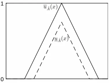
[image:3.612.212.400.126.269.2]uA˜(x)
Figure 1: Interval type–2 fuzzy set.
membership function uA˜ :X →[0,1], where
36
uA˜(x)≤uA˜(x) (1)
for all x∈X. Fig. 1 shows an example of a triangular interval type–2 fuzzy
37
set and its upper (solid) and lower (dashed) membership functions. Fuzzy
38
decision making using type–1 fuzzy sets was introduced by Bellman and
39
Zadeh (1970). Given a set of goals specified by the membership functions
40
{ug1(x), . . . , ugm(x)} (2)
and a set of constraints specified by the membership functions
41
{uc1(x), . . . , ucn(x)} (3)
the optimal decision x∗ is defined as
42
x∗ = argmax
x∈X
ug1(x)∧. . .∧ugm(x) ∧ uc1(x)∧. . .∧ucn(x)
(4)
x∗
0 1
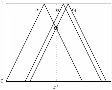
[image:4.612.212.399.123.274.2]g1 g2 c1
Figure 2: Type–1 fuzzy decision.
where ∧is a triangular norm such as the minimum or the product operator.
43
In the experiments presented in section 4 we will use the minimum operator.
44
Fig. 2 shows an example of a type–1 fuzzy decision with two type–1 triangular
45
goals g1, g2 and one triangular constraint c1. Notice that in fuzzy decision 46
making goals and constraints are treated in the same way, so we do not need
47
to explicitly distinguish between goals and constraints.
48
Successful applications of type-1 fuzzy decision making include
environ-49
mental applications such as water resource planning (Afshar et al., 2011) or
50
waste management (Kara, 2011), infrastructure planning applications such
51
as energy system planning (Kaya and Kahraman, 2010) or location
manage-52
ment (Guneri et al., 2009), logistic applications such as supplier selection
53
(Bottani and Rizzi, 2008), transportation planning (He et al., 2012), fuzzy
54
data fusion (Shell et al., 2010) or optimisation of logistic processes (Sousa
55
et al., 2002).
56
In this paper we provide a new fuzzy decision making approach using
terval type–2 fuzzy sets within the context of risk. Chen and Wang (Chen and
58
Wang, 2013, 2011) deploy interval type-2 fuzzy sets to aid decision making
59
through a ranking mechanism and fuzzy multiple attributes decision making.
60
Multi-Criteria Group Decision Making and type-2 fuzzy sets are explored by
61
Naim and Hagras (Naim and Hagras, 2015) in an extensive comparison of
62
different approaches. They are interested in where groups make decisions.
63
Lascio et al. (Di Lascio et al., 2007) take a formal mathematical approach to
64
type-2 fuzzy decision making. Zhang and Zhang (Zhang and Zhang, 2012)
65
extend so called soft sets to type-2 fuzzy sets and provide limited examples of
66
type-2 fuzzy soft sets in decision making. An example application is that of
67
using type-2 fuzzy sets in multi-criteria decision making for choosing energy
68
storage (Ozkan et al., 2015).
69
The decision making research using type-2 fuzzy sets does not align the
70
decision making with the notion of risk. When making a decision our attitude
71
to risk affects our decision making. Our approach then is to consider risk and
72
decision making and provide an interval type-2 fuzzy set approach to that.
73
The rest of the paper is structured as follows: Section 2 provides an
74
overview of interval type-2 fuzzy decision making; Section 3 discusses the
75
properties of this type of decision making; Section 4 provides examples of
76
the use of the approach and Section 5 provides some closing remarks.
77
2. Interval Type–2 Fuzzy Decision Making
78
In type–1 fuzzy decision making the membership values of the goals and
79
constraints quantify the degrees of utility of the different decision options.
80
In interval type–2 fuzzy decision making the utility is subject to uncertainty.
The upper and lower membership values of each option quantify the lower
82
bound (worst case) and upper bound (best case) of the corresponding utility,
83
respectively. Hence, it is straightforward to define the worst case interval
84
type–2 fuzzy decision as
85
x∗ = argmax
x∈X
ug˜1(x)∧. . .∧ug˜m(x) ∧ uc˜1(x)∧. . .∧uc˜n(x) (5)
and to define the best case interval type–2 fuzzy decision as
86
x∗ = argmax
x∈X
ug˜1(x)∧. . .∧ug˜m(x) ∧ uc˜1(x)∧. . .∧uc˜n(x)
(6)
The worst case interval type–2 fuzzy decision maximizes the utility that is
obtained under the worst possible conditions. This decision policy reflects a
cautious or pessimistic decision maker. The best case interval type–2 fuzzy
decision maximizes the utility that is obtained under the best possible
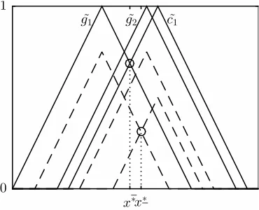
condi-tions. This decision policy reflects a risky or optimistic decision maker. Fig.
3 shows an example of worst case and best case type–2 fuzzy decisions with
two type–2 triangular goals ˜g1, ˜g2 and one triangular constraint ˜c1. We do
not want to restrict the interval type–2 fuzzy decision to the worst case and
best case decisions but we want to allow to specify the level of risk β ∈[0,1]
associated with the decision, where riskβ = 0 corresponds to the worst case
decision x∗ and risk β = 1 corresponds to the best case decision x∗. This
leads us to define the interval type–2 fuzzy decision at risk level β as
x∗β = argmax
x∈X
((1−β)·ug˜
1(x) +β·ug˜1(x))
∧. . .∧((1−β)·ug˜m(x) +β·ug˜m(x))
x∗x∗
0 1
˜
[image:7.612.213.398.125.275.2]g1 g˜2 c˜1
Figure 3: Interval type–2 fuzzy decisions.
87
∧. . .∧((1−β)·uc˜n(x) +β·uc˜n(x))
(7)
It is worth noting the relationship between equations (5) and (6) and the
88
intersection operator. The worst case decision computed in equation (5) may
89
also be calculated through the intersection operator when using the same
t-90
norm as used by the ∧ operator in equations (5), (6) and (7). Equations (5)
91
and (6) find the maximum value across the domain X from the minimum
92
of all the membership functions at a domain point x. This could equally be
93
obtained by finding the highest membership grade across the domain of a
94
fuzzy set which is the intersection of all goals and constraints. Let this fuzzy
95
set f be calculated by equation (8) below.
96
˜
f = ˜g1 ∩. . .∩g˜m∩c˜1∩. . .∩c˜n (8)
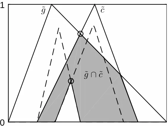
Figure 4 depicts the intersection of a single goal and constraint with the
97
points x∗ and x∗ highlighted by circles. The approach leads to equations (9)
98
and (10) giving alternative ways of calculating the respective worst and best
0
1
˜
g
c
˜
[image:8.612.165.449.127.340.2]˜
g
∩
˜
c
Figure 4: The intersection of an interval type-2 fuzzy goal and constraint
case decisions.
100
x∗ = argmax
x∈X
(˜f(x)) (9)
101
x∗ = argmax
x∈X
(f˜(x)) (10)
We can use equations (9) and (10) to calculate the decision for given risk
102
value β using equation 11.
103
x∗β = argmax(1−β)·µ˜f(x) +β·µ˜f(x))
(11)
whereβ∈[0,1]. The next section explores some properties of this approach.
104
3. Properties of Interval Type–2 Fuzzy Decision Making
105
In this section we investigate in some detail the properties of the interval
106
type–2 fuzzy decision at risk level β defined by (7).
It is easy to see thatx∗0 =x∗ and x∗1 =x∗. It seems reasonable to require
108
that for any risk levelβ ∈[0,1] the decision should be in the interval bounded
109
by the worst case decision x∗ and the best case decisionx∗, so
110
min x∗, x∗≤xβ∗ ≤max x∗, x∗ (12)
for arbitrary t–norms ∧.
111
We now consider whether equation (12) holds for all fuzzy sets, placing no
112
constraints on the membership functions. For simplicity consider a decision
113
with only one goal and no constraint, so for the decision we consider only
114
one single type–2 fuzzy set, and we don’t have to worry about the t–norm
115
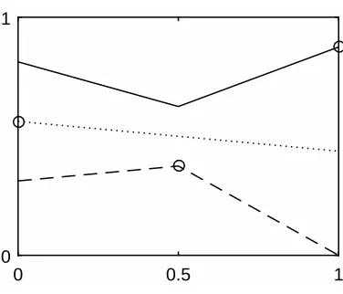
∧. Fig. 5 shows an example of such a type–2 fuzzy set where the maximum
116
of the upper membership function (solid) is at x∗ = 0.5, the maximum of
117
the lower membership function (dashed) is at x∗ = 1, but where for the risk
118
level β = 0.5 (dotted) we obtain the decision x∗0.5 = 0, which is outside the
119
interval between the worst case and the best case, i.e. x∗0.5 6∈ [x∗, x∗]. This
120
example proves that (12) does not hold in general.
121
We will now consider equation (12) for interval type-2 fuzzy set whose
122
membership functions are convex. By convex we mean both the upper and
123
lower membership functions are convex. Consider the two convex interval
124
type-2 fuzzy sets ˜g1 and ˜c1 over the domain X. We know that taking the
125
minimum or the product of two convex functions will always yield a convex
126
function. Therefore ˜g1 ∩c˜1 and ˜g1 ∩c˜1 must yield convex functions when 127
using the product or minimum t-norm. Let ˜f = ˜g1∩c˜1 as with equation(8). 128
It is obvious that the lower membership function of ˜f is contained by the
129
upper membership function of ˜f i.e. f(x)˜ ≥ f(x),˜ ∀x ∈ X. We can now
130
show that (12) holds for convex sets when using the minimum and product
0 0.5 1 0
[image:10.612.211.399.122.283.2]1
Figure 5: Nonconvex example for an interval type–2 fuzzy decision.
t-norms. First divide the domain X into three distinct regions.
132
• Region I: min x∗, x∗≤x≤max x∗, x∗
133
• Region II : x <min x∗, x∗
134
• Region III : max x∗, x∗ < x
135
These regions are depicted in Figure 6. For any value of x∗β to be outside
136
region I it must be in either region II or III. For x∗β to be in region II the
137
derivative of either function must negative with respect to x. Since both
138
functions are convex this is impossible. Forx∗β to be in region III the
deriva-139
tive of either function must positive with respect to x. Since both functions
140
are convex this is impossible. Therefore any value of x∗β must be in region I.
141
This completes the proof.
142
There is a caveat we must add to this discussion which is that x∗β is
143
only non zero when xis in the support of the intersection of all the goals and
144
constraints. If the intersection is an empty set we have no decision agreement.
0
1
I
[image:11.612.164.449.128.343.2]II
III
Figure 6: Regions in a pair of convex functions.
The next section looks at two examples as to how this decision making
146
approach works.
147
4. Application Examples
148
In this section we illustrate our proposed interval type–2 fuzzy decision
149
making approach with two application examples: optimization of the room
150
temperature and choosing optimal travel times with low road congestion.
151
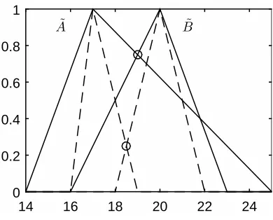
For the first application example assume you have invited two guests, A
152
and B, and wonder to which room temperature you should set the heater.
153
You know that A will be completely happy with 17 degrees, and will be
com-154
pletely unhappy at less than 16 degrees or more than 19 degrees. And B will
155
be completely happy with 20 degrees, and will be completely unhappy for
156
less than 18 degrees or more than 22 degrees. This can be modeled using
14 16 18 20 22 24 0
0.2 0.4 0.6 0.8 1
˜
[image:12.612.208.403.125.282.2]A B˜
Figure 7: Interval type–2 fuzzy decision for the temperature example.
the interval type–2 fuzzy sets shown in Fig. 7, where the upper membership
158
functions for ˜Aand ˜B are shown as solid triangles and the lower membership
159
functions for ˜A and ˜B as dashed triangles. Now a cautious decision maker
160
will set the temperature to 18.5 degrees (lower circle, at the intersection of
161
the lower membership functions, dashed), because then none of the guests
162
will be less happy than 25%. And a risky decision maker will set the
temper-163
ature to 19 degrees (upper circle, at the intersection of the upper membership
164
functions, solid), because in the best case both guests will be 75% happy.
In-165
termediate levels of risk betweenβ = 0 and 1 will yield optimal temperatures
166
between 18.5 and 19 degrees.
167
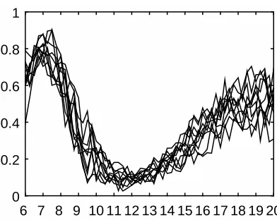
For the second application example assume that we want to drive to work
168
at some time between 6 and 12 o’clock, work for 8 hours, and then drive back.
169
From a traffic reporting system we have obtained the traffic density curves for
170
the 10 previous work days that are shown in Fig. 8. These curves represent,
171
in our view, a sensible view of typical daily traffic density. Note they are non
6 7 8 9 10 11 12 13 14 15 16 17 18 19 20 0
[image:13.612.206.402.123.279.2]0.2 0.4 0.6 0.8 1
Figure 8: Traffic example: Observed traffic densities.
convex and that, as is typical, the uncertainty at the beginning and end of
173
the day is larger.
174
We start with a type–1 fuzzy approach to model this situation and find
175
an optimal decision. Based on the observed traffic densities we estimate
176
the average traffic densities using a mixture of two Gaussian membership
177
functions as
178
u(x) = 0.775·e−(x−1337·60) 2
+ 0.525·e−(x−29019·60) 2
(13)
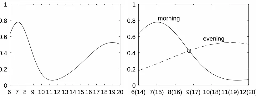
Fig. 9 left shows a plot of this membership function which may be associated
179
with the linguistic label “traffic”, so for example at 7 o’clock we have 0.775
180
traffic. We want to drive to work some time between 6 and 12 o’clock, so for
181
the morning traffic we consider the part of the membership function for the
182
time between 6:00 and 12:00 (solid curve in Fig. 9 right). We want to drive
183
back after 8 hours of work, so for the evening traffic we consider the part
184
of the membership function for the time between 14:00 and 20:00, shifted 8
185
hours to the left (dashed curve in Fig. 9 right). If we do the morning trip
6 7 8 9 10 11 12 13 14 15 16 17 18 19 20 0
0.2 0.4 0.6 0.8 1
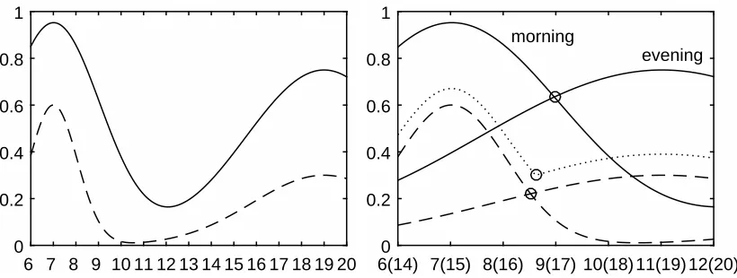
6(14) 7(15) 8(16) 9(17) 10(18) 11(19) 12(20) 0
0.2 0.4 0.6 0.8 1
morning
[image:14.612.113.522.127.283.2]evening
Figure 9: Traffic example: Type–1 fuzzy membership function of the traffic (left) and type–1 fuzzy decision (right).
at 7:00 and the evening trip at 15:00, for example, then we will have 0.775
187
traffic in the morning and about 0.26 traffic in the evening. Our goal is to
188
find a travel time, where the traffic in the morning is low and the traffic in the
189
evening is low. This yields a fuzzy decision with two goals that correspond to
190
the two membership functions shown in in Fig. 9 right. In contrast to the first
191
example we are looking for the minimum, not the maximum memberships,
192
so we replace the argmax in the decision function by argmin. The optimal
193
type–1 fuzzy decision (marked by a circle) is at 8:46 (return 16:46) with a
194
traffic of 0.42 for both the morning and the evening trips.
195
Next, we consider a type–2 fuzzy approach for this problem. We estimate
196
the minimum and maximum bounds of the traffic densities as
197
u(x) = 0.95·e−(x−3·760·60) 2
+ 0.75·e−(x−319·60·60) 2
(14)
198
u(x) = 0.6·e−(x1.5−7··6060) 2
+ 0.3·e−(x4.5−19·60·60) 2
(15)
which represent the lower (dashed) and upper (solid) membership functions
6 7 8 9 10 11 12 13 14 15 16 17 18 19 20 0
0.2 0.4 0.6 0.8 1
6(14) 7(15) 8(16) 9(17) 10(18) 11(19) 12(20)0 0.2
0.4 0.6 0.8 1
morning
[image:15.612.112.522.126.281.2]evening
Figure 10: Traffic example: Interval type–2 fuzzy membership function of the traffic (left) and type–2 fuzzy decision (right).
of the interval type–2 fuzzy membership function of the traffic, as shown in
200
Fig. 10 left. The lower and upper membership functions for both the morning
201
and evening trips are shown in Fig. 10 right. The three circles show three
202
type–2 fuzzy decisions at different risk levels. A cautious decision maker will
203
drive to work at 8:59 and back at 16:59 (upper circle), because the worst case
204
traffic is about 0.64. A risky decision maker will drive to work at 8:32 and
205
back at 16:32 (lower circle), because the best case traffic is about 0.22. For
206
intermediate levels of risk the optimal decision will be to leave between 8:32
207
and 8:59 and return 8 hours later. For example, for risk level β = 0.8 we
208
obtain the dotted curve which is minimized for leaving at 8:37 and returning
209
at 16:37 with a traffic of about 0.3.
210
A comparison of the type–1 and type–2 fuzzy decisions is shown in Fig. 11.
211
The two almost linear solid curves show the worst case and best case traffic
212
for the morning trip times between 8:30 and 9:00, corresponding to evening
8:30(16:30) 8:45(16:45) 9:00(17:00) 0
0.2 0.4 0.6 0.8 1
best case worst case
type 1 8:46(16:46) min type 2
8:32(16:32)
max type 2 8:59(16:59)
-5.3%
[image:16.612.195.418.124.283.2]-8.1%
Figure 11: Traffic example: Comparison of the worst case and best case traffic for the type–1 and type–2 fuzzy decisions.
trip times between 16:30 and 17:00. The middle dashed line at 8:46(16:46)
214
corresponds to the type–1 fuzzy decision, where the worst case traffic is about
215
0.69 and the best case traffic is about 0.23. The left dashed line at 8:32(16:32)
216
corresponds to a risky decision maker who picks the minimum type–2 fuzzy
217
decision, where the best case traffic is 5.3% lower than the best case for the
218
type–1 fuzzy decision. The right dashed line at 8:59(16:59) corresponds to
219
a cautious decision maker who picks the maximum type–2 fuzzy decision,
220
where the worst case traffic is 8.1% lower than the worst case for the type–1
221
fuzzy decision. So if we specify a risk level that we are willing to accept, then
222
type–2 fuzzy decision making can take this risk level into account and may
223
therefore yield better results than type–1 fuzzy decision making.
5. Conclusions
225
Existing approaches supporting decision making using type-2 fuzzy sets
226
ignore the risk associated with these decisions. In this paper we have
pre-227
sented a new approach to using interval type–2 fuzzy sets in decision making
228
with the notion of risk. The method extends the work of Bellman and Zadeh
229
(1970) by replacing the type–1 fuzzy sets with interval type–2 fuzzy sets.
230
This brings an extra capability to model more complex decision making, for
231
example, allowing trade-offs between different preferences and different
atti-232
tudes to risk. The explicit consideration of risk levels increases the solution
233
space of the decision process and thus enables better decisions. In a traffic
234
application example, the quality of the obtained decision could be improved
235
by 5.3–8.1%.
236
The paper explores some of the properties of this new approach and with
237
two examples shows how it works. We will follow on this work by tackling
238
larger, more complex, problems as well as investigating the properties in more
239
detail.
240
References
241
Afshar, A., Mari˜no, M. A., Saadatpour, M., Afshar, A., 2011. Fuzzy TOPSIS
242
multi-criteria decision analysis applied to Karun reservoirs system. Water
243
Resources Management 25 (2), 545–563.
244
Bellman, R., Zadeh, L., 1970. Decision making in a fuzzy environment.
Man-245
agement Science 17 (4), 141–164.
Bottani, E., Rizzi, A., 2008. An adapted multi-criteria approach to
suppli-247
ers and products selection an application oriented to lead-time reduction.
248
International Journal of Production Economics 111 (2), 763–781.
249
Chen, S.-M., Wang, C.-Y., 2013. Fuzzy decision making systems based on
250
interval type-2 fuzzy sets. Information Sciences, Volume 242, 1 September
251
2013, Pages 1-21, ISSN 0020-0255.
252
Chen, S.-M., Wang, C.-Y., 2011. A new method for fuzzy decision making
253
based on ranking generalized fuzzy numbers and interval type-2 fuzzy sets.
254
Machine Learning and Cybernetics (ICMLC), 2011 International
Confer-255
ence on, Guilin, 2011, pp. 131-136.
256
Di Lascio, L., Fischetti, E., Gisolfi, A., Gisolfi, A., and Nappi, A., 2011.
Type-257
2 fuzzy decision making by means of a BL-algebra. IEEE International
258
Fuzzy Systems Conference, London, 2007, pp. 1-6.
259
Guneri, A. F., Cengiz, M., Seker, S., 2009. A fuzzy ANP approach to shipyard
260
location selection. Expert Systems with Applications 36 (4), 7992–7999.
261
He, T., Ho, W., Man, C. L. K., Xu, X., 2012. A fuzzy AHP based integer
262
linear programming model for the multi-criteria transshipment problem.
263
The International Journal of Logistics Management 23 (1), 159–179.
264
Gehrke, M., Walker, C., and Walker, E., 1996. Some comments on interval
265
valued fuzzy sets. Int. J. Intell. Syst., vol. 11, pp. 751–759.
266
Gorzalczany, M. B., 1987. A method of inference in approximate reasoning
267
based on interval-valued fuzzy sets. Fuzzy Sets and Systems Volume 21,
268
Issue 1, January 1987, Pages 1–17.
Kara, S. S., 2011. Evaluation of outsourcing companies of waste electrical
270
and electronic equipment recycling. International Journal of
Environmen-271
tal Science & Technology 8 (2), 291–304.
272
Kaya, T., Kahraman, C., 2010. Multicriteria renewable energy planning using
273
an integrated fuzzy VIKOR & AHP methodology: The case of Istanbul.
274
Energy 35 (6), 2517–2527.
275
Liang, Q., and Mendel, J. M., 2000. Interval type-2 fuzzy logic systems:
276
Theory and design. IEEE Trans. Fuzzy Syst., vol. 8, no. 5, pp. 535–550.
277
Malek, M., Tumeo, M., and Saliba, J., 2015. Fuzzy logic approach to risk
278
assessment associated with concrete deterioration. ASCE-ASME Journal
279
of Risk and Uncertainty in Engineering Systems, Part A: Civil Engineering,
280
1(1):04014004, 2015.
281
Mays, M. D., Bogardi, I., and Bardossy, A., 1997. Fuzzy logic and risk-based
282
soil interpretations. Geoderma Volume 77, Issues 2–4, June 1997, Pages
283
299–315.
284
Mendel, J. M., John, R. I., and Liu, F., 2006. Interval type-2 fuzzy logic
285
systems made simple. Fuzzy Systems, IEEE Transactions on, 14(6):808–
286
821.
287
Naim, S., and Hagras, H., 2015. A Type-2 Fuzzy Logic Approach for
288
Multi-Criteria Group Decision Making. Granular Computing and
Decision-289
Making: Interactive and Iterative Approaches, Springer International
Pub-290
lishing Editor Pedrycz, W., and Chen, S.-M., 123–164
¨
Ozkan, B., Kaya, ˙I., Cebeci, U., and Ba¸slıgil, H., 2015. A Hybrid
Multi-292
criteria Decision Making Methodology Based on Type-2 Fuzzy Sets For
293
Selection Among Energy Storage Alternatives. International Journal of
294
Computational Intelligence Systems Vol. 8, Iss. 5.
295
Runkler, T. A., Coupland, S., and John, R., 2015. Properties of interval
296
type-2 defuzzification operators. IEEE International Conference on Fuzzy
297
Systems, pp 1–7.
298
Shell, J., Coupland, S., and Goodyer, E., 2010. Fuzzy data fusion for fault
299
detection in wireless sensor networks. Computational Intelligence (UKCI),
300
2010 UK Workshop on, pages 1–6.
301
Sousa, J. M., Palm, R., Silva, C. A., Runkler, T. A., 2002. Fuzzy optimization
302
of logistic processes. In: IEEE International Conference on Fuzzy Systems.
303
Honolulu, pp. 1257–1262.
304
Zadeh, L. A., 1965. Fuzzy sets. Information and Control 8, 338–353.
305
Zadeh, L. A., 1975. The concept of a linguistic variable and its application to
306
approximate reasoning. Information Science 8, 199–250, 301–357, 9:42–80.
307
Zhang, Z., and Zhang, S., 2012. Type-2 Fuzzy Soft Sets and Their
Appli-308
cations in Decision Making, Journal of Applied Mathematics, vol. 2012,
309
Article ID 608681, 35 pages, 2012.