Abstract—The Dynamic Phasor (DP) concept has been widely used in modelling electrical power systems. So far, the DP concept has been restricted to modelling systems with one single electrical source at a fixed fundamental frequency; either one generator or an ideal three-phase AC source. This paper aims to extend the DP modelling methodology to a wider application area. Two major achievements have been introduced: 1. application of DPs for multi-source, multi-frequency systems; 2. modelling of systems with time-varying frequencies. These two techniques enable the use of DPs to study nearly all types of Electrical Power Systems (EPS). The developed theory is validated using a twin-generator system from the More Open Electrical Technologies (MOET) project. The accuracy and effectiveness of the developed models is confirmed by comparing the simulation results of detailed switching models and DP models under both balanced and unbalanced conditions.
Index Terms— more-electric aircraft, dynamic phasors, modelling, multi-source, multi-frequency, time-varying frequency
I. ABBREVIATIONS
ATRU Auto-Transformer Rectifier Unit APU Auxiliary Power Unit
DP Dynamic Phasor
ECS Environment Control System EMA Electro-Magnetic Actuator EPS Electrical Power Systems
FTC Frame Transformation Coefficient GCU Generator Control Unit
HVDC High-Voltage Direct Current HVAC High-Voltage Alternative Current MEA More Electric Aircraft
MOET More Open Electrical Technology PEC Power Electronic Converter PMM Permanent Magnet Machine SG Synchronous Generator WIPS Wing Icing Protection System
II. INTRODUCTION
With the advancement of power electronics and control theory, there has been significant penetration of power electronics into Electrical Power Systems (EPS) in recent years. This includes within applications such as the modern electric
grid, distributed energy resources and the electrical systems of ships, aircraft and vehicles. However, increased system complexity and a wide variation in the time scales of electromagnetic and electromechanical phenomena in the system will lead to significant challenges for EPS designers [1]. Modelling and simulation of these power electronic based systems is thus essential to design and verify the developed energy systems [2].
Traditionally, the dynamic behaviour of EPS can be studied using models created in commercial software such as Saber, Matlab/Simpower, etc. [3-5]. These models usually include detailed switching behaviour of semiconductor devices. When studying large-scale EPS, the application of these switching models often leads to significant computing time as well as large computer storage requirements. In addition, the switching models are discontinuous and thus difficult to extract the small-signal characteristics for system-level studies [2].
Since the switching behaviour of Power Electronic Converters (PECs) has little added value for system-level studies, a number of approaches have been exploited to balance the accuracy and efficiency of the models. Averaging the variables during one switching period, the dynamic average model, has been widely used and proved to be an efficient method to model PECs. However, the publications available mainly focus on the modelling of PECs under balanced conditions [2, 6-8]. For unbalanced conditions, the complex behaviour of switching functions of PECs makes it difficult to develop the average models with high accuracy. For three-phase EPS, the average model is based on the Park transformation which transfers the quantities in the three-phase coordinate (ABC frame) into a synchronous rotating dq frame. This technique is also referred to as the DQ0 average modelling technique. These average models have shown great performance for EPS studies during balanced operation [9-11]. However, for unbalanced and faulty regimes this technique loses its efficiency and is time-consuming due to the second harmonic in the d and q axes [12].
An alternative approach that can address this problem is to use Dynamic Phasor (DP) models, also referred to as the general averaging model [13]. DPs are essentially time-varying Fourier series coefficients. This method can model the fundamental component as well as higher harmonics in the system. Under both balanced and unbalanced conditions, the DP variables are constant or slow-varying complex quantities which allow big time steps during the simulation process.
Dynamic Phasor Modelling of Multi-Generator
Variable Frequency Electrical Power Systems
T. Yang, S. Bozhko,
Member, IEEE,
J.M. Le-Peuvedic, G. Asher,
Fellow, IEEE,
The DP technique has been successfully used in modelling a number of electrical and electronic devices, such as electrical machines [14-16], power system dynamics and faults [17], flexible AC transmission systems [18, 19], sub-synchronous resonance [20], dc-dc converters [21] and High-Voltage Direct Current (HVDC) systems [22]. For system-level studies, the single machine infinite bus has been studied with DPs [17], where all the generators were perfectly synchronized and operating at a common fixed fundament frequency. However, this is not always true in the real world. In fact, many applications require variable frequency or generators with multiple frequencies. For example; the electrical output frequency of a generator which is time varying during start up and shut down, the typical oscillations that occur in the synchronous machines of a conventional grid with frequencies of 0.1-4Hz, and the EPS in future aircraft as these will be supplied by variable frequency generators with a common HVDC bus.
This paper aims to establish a foundation for DP modelling of multi-generator, multi-frequency systems as well as systems with time-varying frequencies. The paper is organized as follows: the DP concept is introduced in Section II; Section III develops the theory of DP modelling of time-varying frequency systems; the theory of DP modelling of multi-generator multi-frequency systems is introduced in Section IV; the implementation of the developed theory is demonstrated using a twin-generator aircraft EPS in Section V, which is followed by the paper’s conclusions in Section VI.
III. DYNAMIC PHASOR CONCEPT
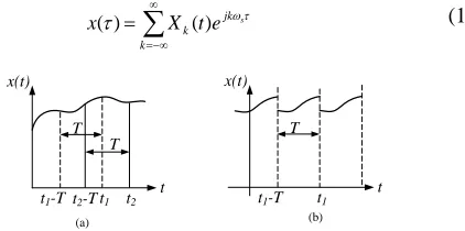
The DP concept is based on the generalized averaging theory and was first reported in [13]. DPs are essentially time-varying Fourier coefficients. For a time-domain quasi-periodic waveform x(τ), defining a time-moving window τ(t-T, t], as shown in Figure 1, and viewing the waveforms in this window to be periodic, the Fourier expansion of the waveform in this interval can be represented by the following Fourier series:
k
jk k
s
e t X
x() () (1)
t1-T t1 t2
T T x(t)
t
t1-T t1
T x(t)
t
(a)
t2-T
(b)
Figure 1 (a) Defined moving window at time t1 and t2, (b) equivalent periodic signal at time t1
where ωs=2π/T and T is the length of the window. Xk(t) is the kth Fourier coefficient in a complex form and is referred to as a “Dynamic Phasor” (DP). It is defined as follows:
k
t
T t
jk
k x e d x
T t
X
s
) ( 1 )
( (2)
A key factor in developing dynamic models based on DPs is the relationship between the derivatives of the variable x(τ) and the derivatives of the kth Fourier coefficient given as:
) ( )
( )
( jk X t
dt t dX t dt dx
k s k
k
(3)
This can be verified using (1), (2), and be used in evaluating the
kth phasor of time-domain model. The differential term on the right side of (3) is crucial, since this term represents the transient dynamic of variables. Dropping this term, the differential property of DPs reduces to be the same as that of traditional phasors. This property will also be modified when
ωs is time-varying and will be discussed in section IV. Another important property of DPs is that the kth phasor of a product of two time-domain variables can be obtained via the convolution of corresponding DPs:
i k i i
k x y
xy (4)
The properties (3) and (4) play a key role when transforming the time-domain models into DP domain. Algebraic manipulations in this paper will also exploit the following property of real functions x(τ):
) ( ) (t X*t
Xk k (5) where the notation ‘*’ denotes a complex conjugate. Applying (5), the real time-domain waveform can be derived from (1) and rewritten as:
1
0() 2 ()
) (
k
t jk k
s
e t X e t
X t
x (6)
Transforming (1) into the frequency domain gives
k
s
k j jk
X j
X( ) ( ) (7)
As seen in (7), applying the DP concept shifts all the band limited components at kωs by –kωs. This makes all the harmonics become base-band components, as illustrated in Figure 2, and allows bigger simulation steps and higher computation efficiency.
) ( X
s
2s
s
s
3
2s 3s
)
( s
kj k
X
0
To DPs
) (
1
X X3() )
(
1
X
) (
3
X
[image:2.612.84.295.509.614.2] [image:2.612.357.522.538.658.2]IV. DYNAMIC PHASOR MODELLING OF VARYING FREQUENCY WAVEFORMS
So far, all the DPs are constant frequency. As mentioned before, there is no system with a perfectly fixed frequency. Even in a conventional grid, it is typical that an oscillation with a frequency of 0.1-4Hz is manifested in the synchronous machines. The application of DPs in modelling time-varying frequency systems has been touched on in [13]. There, the author chooses a ‘sliding window’ with phase angle θ(t)=2π for the time-varying frequency signals. The theory developed in [13] is difficult for application and there has been no further development in this area since [13]. In this section, the authors propose another methodology that makes the application of DPs in modelling time-varying EPS convenient.
As briefly highlighted in section II, the analysis based on (2) is valid if ωs is constant. In the case where the frequency ωs is time varying, the selection of a ‘time-moving window’ in the DP definition should be reconsidered. The main difficulty of DPs of time-variant frequency waveforms is to derive the differential of a DP when ωs varies. For a waveform with a time-varying frequency, it is convenient to define the DP using the phase angle θ instead of the angular speed ωs as was used in (2). Using the phase angle θ, the DP definition becomes:
,... 2 , 1 , 0 )) ( ( 2 1 2
k d e t x x jk k (8)
where
t s d
t
0 ( )
)
(
(9) This approach was reported in [13] where the author derived the derivative property as:
2 ) ( ) ( ) ( ) ( ) ( ) ( 2 1 ) ( ) ( ) ( 2 1 ) ( ) ( d t jk t t e t x t T t T t e t T t x dt t x d dt t dx t jk t T t jk k k (10)
The proof of (10) is shown in [13] and will not be detailed in this paper. As can be seen above, when the frequency is constant, i.e. ω̇ (t)=0 and Ṫ (t)=0, (10) will reduce to (3). However, for the case of ω̇ (t)≠0, equation (10) is extremely complicated and this makes its implementation totally impractical. Therefore in reality, it is not possible to use (10) to study EPS. This is due to the fact that the two terms x(t-T(t)) and ω(t-T(t)) require the solver to store all the results during the
T(t) period, for a large-scale EPS with many state variables, it will result in impractical computation time. Indeed, after the authors reveal (10) in [13], DPs have never been used in literature for time-varying frequency systems.
In this paper, we introduce an alternative approach to derive a simple formula for the DP of the differential term and this is:
k k k x t jk dt x d dt dx ) (
(11)
Proof: To prove this result, it must first be recalled that according to the definition in (8), the differential of DP 〈x〉k can be expressed as:
2 ( ) 2
1 )
(
k jk
k e t x t dt d d x d dt x
d (12)
In addition, the DP form of a differential term dx dt⁄ can be given as:
2 2 )) ( ( 2 1 )) ( ( 2 1 d e dt d d t dx d e dt t dx dt dx jk jk k (13)Since dθ/dt=ω(t), (13) can be written as:
2 )) ( ( ) ( 2 1 t dx e t dt dx jk k (14)Then exchanging the integration terms in (14) yields:
2 2
)) ( ( 2 1 ) ( ) ( )) ( ( 2 1 d e x t jk e t t x dt
dx jk jk
k
(15)
The first term, from (12) is equal to d‹x›k/dt. The second term, from (8) is equal to jkω(t)‹x›k. Therefore, combining (8), (12) and (15) gives (11).
Comparing (11) and (3), one can notice that the derivative characteristics of frequency based DP and phase angle based DP are of the same form. This implies that these two types of DPs can be treated equally.
V. MULTI-FREQUENCY SYSTEMS MODELLING WITH DYNAMIC PHASORS
In addition to DP modelling of time-varying frequency EPS, another issue addressed in this paper is the DP modelling of EPS with multiple frequencies, i.e. multiple generators. EPS with multiple generators working in parallel are very common for redundancy and safety reasons. Taking the Airbus A380 as a prime example, there are four main generators and an Auxiliary Power Unit (APU) in the EPS. During the engine start-up and shutdown process of the aircraft, there is a transition between the aircraft electrical power being supplied by the APU and the main generators. During this transition multiple generators are running in parallel at differing frequencies. In this section, the DP modelling technique will be extended to modelling multi-generator parallel-operation systems. A common reference frame, called the master frame, is chosen in the multi-generator system and all the variables in the model are referred to the master frame. It will be seen later in this section, that the transformation between different frames can be represented with some simple algebraic functions. This is extremely convenient when implementing the theory developed in this section.
For the same time-domain waveform, the DP transformation with different base frequencies, will define distinct series of DPs. Let a time-domain waveform xq(t) be associated with the
qth Synchronous Generator (SG) with a base frequency ωq. Then the DP of xq(t) can be written as:
... 2 , 1 , 0 , ) ( 1 ) (
n d e x T t X t T t jn q q qn q q
where ωq=2π/Tq. The first subscript ‘q’ in Xqn(t) denotes that the DP is associated with the variable xq(t) and the qth generator with a base frequency ωq. The second subscript ‘n’ gives the DP index in this frame. To proceed, we define a master frame or primary frame with base frequency ωp and the DPs for the signal xq(t) in this frame can be written as:
... 2 , 1 , 0 , ) ( 1 ) (
m d e x T t Y t T t jm q p pm p p
(17)where ωp=2π/Tp. The ‘m’ gives the DP index in the corresponding ωp frame. In this paper, the DPs in their own frame are denoted using ‘X’ and the DPs after frame
transformation are denoted with ‘Y’. A linear relation between
DPs in the master frame (ωp frame), and the slave frame (ωq frame) can be written as:
... 2 , 1 , 0 , ) ( )
(t
C e X t mY n qn t j nm pm nm
(18)
The proof of (18) is shown in Appendix I. In (18),
∆ωnm=nωq-mωp and the coefficient Cnm is dependent on ∆ωnm. Using (18), transformation from DPs in the master ωp frame to DPs in the slave ωq frame can be achieved. In this case, every component of Xqn(t) will contribute to a widespread range of
Ypm(t) (m=0, 1,2, …). However, this study is focused on the functional modelling level [10] and as such we neglect high harmonics and only the fundamental component is considered. Thus all signals are represented by their fundamental components.
Applying:
) cos( )
(t A t
xq q (19) Let the base frequency ωq, then the DP Xqn(t) can be calculated as: 1 0 1 5 . 0 ) ( n n Ae t X j qn (20)
From (20), it can be concluded that in the ωq frame, all the DPs except Xq1(t) (n=1) are equal to zero. Using (18) and (20), the DPs in the master frame are written as:
) ( )
( 1 1
1 X t
e C t Y q t j m pm m
, m=1, 2, … (21) Therefore, it can be seen from (20) and (21), that in the slave frame, Xqn(t) only includes the DP component with n=1. However, when transferred into the master frame,
Ypm(t) includes a series of DPs with a wide range of frequency components (m= 1, 2,…). This makes the frame transformation difficult to calculate and impractical for applications. To make progress, we utilise the fact that in the slave frame, the DPs of
xq(t) only include the n=1 component, as shown in (20). From (21), we can define the complex variable Ypm' (t) as:
) ( ) ( 1 1 ' t Y C t
Ypm m pm
, m=1, 2,… (22) Combining (21) and (22) gives:
) ( )
( 1
' t e 1 X t
Y q t j pm m
, m=1, 2,… (23) Equation (22) illustrates a linear relation between Yp'm(t) and
Ypm(t). This indicates that Ypm ' (t) is still in the master frame. Equation (23) reveals that the DP Ypm' (t) can be derived from a rotational transformation of the DP Xq1(t), with rotating angle γ=∆ω1mt=(ωq-mω1)t.
From (20), we know that Xq1(t) includes all the information for the sinusoidal xq(t). While, equation (23) reveals that Ypm ' (t) is derived from a rotational transform of Xq1(t). It can therefore be concluded that each item of Ypm ' (t) (m=1,2,…) contains all the required information needed for xq(t). Indeed, considering the case m=1 in (23) gives:
) ( ) ( 1 ' 1
11X t
e t
Yp j t q (24) Combining (6) and (24) the time-domain waveform xq(t) can be traced back from Yp1 ' (t) with
j t
p t j t j p t j q q p q q e Y e e e Y e e t X e t x ' 1 ' 1 1 2 2 ) ( 2 ) (
11
(25)
where the function Re derives the real term of the complex variable. Equations (24) and (25) illustrate that the complex variable Yp1 ' (t) can be used as a DP in the master frame. The DPs in those two different frames are related with a rotating function ej∆ω11t, as shown in (24). The introduction of this extra complex variable Yp1 ' (t) makes the frame transformation more convenient and mathematically easier for application.
2 d Load system1 Load system2 Load system q (26) (26) Subsystem in the ω1 frame
[image:4.612.369.513.433.606.2]SG1 SG2 2 d SGj ωp ωk ωq nm ) ( 1t Xv p ) ( 1t Xi p ) ( 1t Xv q ) ( 1t Xi q ) ( 1t Yv p ) ( 1t Yi p ) ( 1t Xv p ) ( 1t Xi p
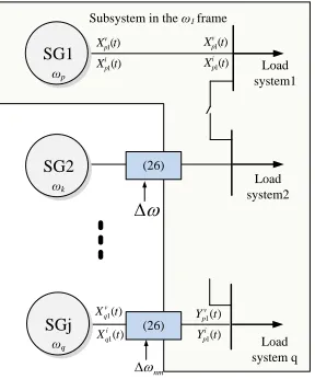
Figure 3 DP modelling of multi-generator systems
The application of (24) can be illustrated using a multi-generator system as shown in Figure 3. The synchronous generator SG1, with rotating frame ωp, is selected as the master frame. Other generators SGj (j≠1) are viewed as slave
be developed to connect a itslave-frame based DP subsystem with a master-frame based DP subsystem using:
) (
) (
) ( '
) ( '
1 1
1 1
1 1
t X
t X e t Y
t Y
i p v q t j i
p v
p (26)
where Xq1𝑣(t), Xq1𝑖 (t) are DPs of the voltages and currents in the slave frame and Yq1′𝑣(t), Yq1′𝑖(t) are the DPs in the master frame after transformation.
VI. IMPLEMENTATION
Two test cases are presented in this section. The first case is used to validate the application of the phase-based DPs in modelling frequency-varying systems. This is validated experimentally. The second case applies the DP frame transformation theory to a twin-generator EPS in a More-Electric Aircraft (MEA). The results from DP models are compared with those from detailed behavioural models (referred to as ABC models). The DP models of EPS elements can be found in our recent publications [23-25]. Simulations have been performed on an Intel i7 [email protected], 24.0GB of RAM using Modelica/Dymola v.7.4 software. The Radau IIa algorithm has been chosen in the solver and the tolerance has been set at 1e-4. As a quantitative evaluation of the computation efficiency, the computation time has been compared between DP and ABC models.
A. Application of phase-based DPs
The proposed phase-based DPs will now be validated experimentally. The scheme for testing is shown in Figure 4. A three-phase power supply with internal impedance Rs and Ls is used to supply an RL load. The California MX45 is used as the AC power supply. When running as an AC source, the MX45 has internal impedance of Rs= 50mΩ and Ls=200μH. The load resistance is R=57.2Ω and inductance is L=0.8mH. In this test, a step change of frequency from 50Hz to 400Hz is applied to the system. This step change will rarely happen in a generator driven system. However, this extreme case provides a good test to validate the developed theory. In order to trigger the scope, the magnitude of AC power is also stepped from 20Vrms to 40Vrms.
A
B Rs
C Ls
Va
Vb
Vc
R L
R L
R L
AC power supply
[image:5.612.327.551.393.586.2]
(a) (b)
[image:5.612.52.298.574.679.2]Figure 4 Validation of varying frequency DPs. (a) system configuration; (b) test rig
Figure 5 Phase A currents flowing through resistor R comparison between DP model and experimental results with frequency steps from 50Hz to 400Hz
The load currents (phase A) from the DP models are transformed to the time-domain and compared with the experimental results, as shown in Figure 5. The experimental results, and those from phase-based DP model, are almost identical before and after step change in frequency. This therefore confirms the accuracy of phase-based DP in modelling time-varying frequency systems.
B. Twin-generator system
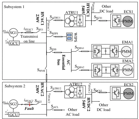
A twin-generator electrical power system of MEA is shown in Figure 6. This large aircraft hybrid AC/DC power system is based on an A380 style EPS and was the subject of studies within More-Open Electrical Technologies (MOET) project [10].
SG1
GCU
SATRU1
PMM
PMM
W
IP
S
SATRU2
SACL
Other AC load
PMM Other
DC load ECS1
SG2
GCU
SHVB
H
V
A
C
1
2
3
0
V
H
V
A
C
2
2
3
0
V
H
V
D
C
1
5
4
0
V
Other DC load
H
V
D
C
2
5
4
0
V
*
T
v
ωe2 * T
v
EMA1 ωe1
EMA2 SECS1
PMM ECS2 SECS2
SWIPS
SESS
iHVAC1 SSG1
SSG2
A
C
E
ss
en
tia
l
b
u
s
SEMA1
SEMA2
ATRU1
ATRU2 Subsystem 1
Subsystem 2
Fault
Transmissi on line
v
H
V
D
C
2
iHVAC2
v
H
V
D
C
1
v
H
V
A
C
1
v
H
V
A
C
2
Figure 6 One twin-generator electrical power system of MEA
The main elements of the EPS in Figure 6 include the Synchronous Generator (SG) and its control unit, Auto-Transformer Rectifier Units (ATRUs), Wing-Ice Protection System (WIPS), Environmental Control System (ECS) and Electro-Mechanical Actuators (EMAs). The Generator Control Unit (GCU) is used to control the voltage of the main AC bus. The ATRUs provide AC to DC power conversion. They are comprised of an auto-transformer and three sets of diode bridges [26]. The WIPS is an electrical de-icing system. It is modelled as a three-phase variable
0.01 0.02 0.03 0.04
-1.5 -1 -0.5 0 0.5 1 1.5
Time(s)
Cu
rre
n
t
ia
(A
)
Exp DP
resistive load. The ECS system is driven by large compressors which are modelled as Permanent Magnet Machines (PMMs). The ECS provides environmental temperature control and cabin pressurization. The EMAs, which are mainly used for the flight control actuation, consist of an electric motor and gear box assembly and are modelled as PMMs fed by back-to-back inverters.
1) Normal Operation Conditions
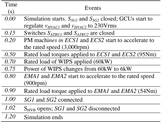
[image:6.612.342.529.234.387.2]This section presents simulation studies of the power system in Figure 6 under start-up and normal conditions. During the start-up process, the two subsystems operate independently. It is assumed that the generators have reached the rated speed before the electrical system starts operation. The electrical frequencies of synchronous generators SG1 and SG2 are fixed at 400Hz and 405Hz respectively with different initial rotor angles. This asynchronism represents a real situation where the two generators are driven by different engine shafts. After the generators reach steady state, a series of events occurs. The event sequence during start-up of the twin-generator aircraft EPS is shown in Table I.
TABLE I EVENTS SEQUENCE OF MEA TWIN-GENERATOR SYSTEM CASE
Time
(s) Events
0.00 Simulation starts. SSG1 and SSG2 closed; GCUs start to regulate vHVAC1 and vHVAC2 to 230Vrms
0.15 Switches SATRU1and SATRU2 are closed
0.20 PM machines in ECS1 and ECS2 start to accelerate to the rated speed (3,000rpm)
0.50 Rated load torques applied to ECS1 and ECS2 (95Nm)
0.70 Rated load of WIPS applied (60kW)
0.75 Power of WIPS changes from 60kW to 6kW
0.80 EMA1 and EMA2 start to accelerate to the rated speed (900rpm)
0.90 Rated load torque applied to EMA1 and EMA2 (54Nm)
1.00 SG1 and SG2 connected
1.02 SHVB opens; SG1 and SG2 disconnected
1.20 Simulation ends
Results from the ABC and DP models are compared in the following figures. The dynamic responses of the DC bus voltages, vHVDC1 and vHVDC2 are shown in Figure 7. It can be seen that the voltage vHVDC1 and vHVDC2, from two different modelling techniques, match very well. Since the initial values of vHVDC1 and vHVDC2 are set at zero, when the switches SATRU1 and SATRU2 are closed, vHVDC1 and vHVDC2 jump from 0V to around 800V. This is due to the inrush of current charging the zero-initialized capacitor. When generators SG1 and SG2 are connected, vHVDC1 and vHVDC2 drop due to the difference between vHVAC1 and
vHVAC2. When the two generators disconnect at t=1.02s, the two subsystems return to their previous steady state before parallel operation. SG2 then starts to supply the whole load system and the system settles into steady state after a short transient period.
Since the system is assumed to be balanced, the currents flowing into the ATRU iATRU1 are represented by the phase A current only. For comparison, the variables in the DP models are transformed into three-phase coordinates within the time domain, as shown in Figure 8. The magnitudes of the DPs, denoted by |DP|, are also shown in these figures. As can be seen, the currents iATRU1 remain at zero until the load is connected to the HVDC buses. At 0.2s the acceleration of the PMMs in the ECS causes increased current in iATRU1. The application of rated ECS load causes another step response in
[image:6.612.39.312.344.546.2]iATRU1 at t=0.5s. Again, it can be seen that the results from the ABC and DP models are well matched during the whole simulation process. The DP magnitudes form envelops of the time-domain currents iATRU1.
Figure 7 The dynamic response of vHVDC1 and vHVDC2. Above: response of vHVDC1; below: response of vHVDC2
0 0.2 0.4 0.6 0.8 1 1.2
-200 0 200
iAT
R
U
1
(A
)
0.96 0.98 1 1.02 1.04
-150 -50 50 150
Time(s)
iAT
R
U
1
(A
)
ABC DP |DP|
magnitude of DPs
SGs connect SG1 removes ECS1 speed up
Loads on ECS1
WIPS reudction
0.787 0.7875 0.788 0.7885 0.789 0.7895 -60
-40 -20 0 20 40 60
Figure 8 The dynamic response of iHVAC1, phase A current flowing into ATRU1. Above: iHVAC1; below: zoom-in area of iHVAC1
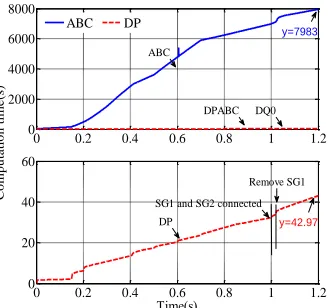
The computation time consumed by the three models is compared in Figure 10 and in Table II. It can be seen that the DP model is 185 times faster than the ABC model.
0 0.2 0.4 0.6 0.8 1
0 200 400 600 800 1000
vH
V
D
C
1
(V
)
0 0.2 0.4 0.6 0.8 1
0 200 400 600 800 1000
Time(s)
v H
V
D
C
2
(V
)
ABC DP
ECS2 Loads on
ECS2 speeds up
Accerlation Finished
ECS1 Loads on
ECS1 speeds up
Accerlation Finished WIPS
[image:6.612.337.533.431.582.2]Figure 9 Comparison of the computation time between three different models
TABLE II COMPARISON OF THE COMPUTATION TIME BETWEEN THREE DIFFERENT MODELS
Model ABC DP
Simulation time (s) 7983.00 42.97
Acceleration factor 1 185
2) Line-to-Line Fault Conditions
The application of DPs in modelling EPS in faulty conditions has been discussed in [24, 25, 27]. In these publications, the DP modelling technique was used to model synchronous generators, ATRUs, front-end rectifier units, diode bridges and transmission lines. All of the developed models were tested under both balanced and unbalanced conditions. In this section, the system behaviour under line-to-line fault conditions will be studied. The line-to-line fault is imposed between phase A and phase B at the transmission line connecting the generator SG2 and the HVAC1 bus, as shown in Figure 6. The fault is implemented by using a 0.1mΩ resistor between the phases. The system goes through a series of events the same as those shown in Table I, prior to the line-to-line fault occurring at t=1.2s. Since the fault happens at the main AC supply cables, all the elements in the EPS will be fed by severely distorted power during the fault condition.
Table III SIMULATION SCENARIOS OF TWIN-GENERATOR AIRCRAFT EPS UNDER ABNORMAL OPERATION CONDITIONS
Time (s) Events
…. Same as Table I
1.20 A line-to-line fault occurs between the SG2 and
the HVDC2 bus
1.30 Simulation ends
Figure 10 The dynamic response of HVDC bus voltages, vHVDC1 and vHVDC2, with a line-to-line fault occurring at t=1.2s.
Figure 11 The dynamic response of currents flowing into the ATRU2 with a line-to-line fault occurring at t=1.2s
Figure 10 shows the DC-link voltages of ATRU1 and ATRU2. After the fault occurs, vHVDC1 and vHVDC2 reduce from 540V to a new steady state around 310V. The power quality of the DC side is reduced and the apparent harmonics can be due to the increased voltage ripple, as shown in Figure 10. The currents flowing into the ATRU2 are shown Figure 11. The results from the DP model are transformed into three-phase coordinates within the time domain for comparison studies. It can be seen from Figure 11 that after fault occurs, the AC currents flowing into the ATRUs are distorted. The results from the two different modelling techniques are well matched both before and after the fault occurs. The computation time of different models is shown in TABLE IV. As can be seen, the DP model in this case is almost 90 times faster than the ABC model.
TABLE IV COMPARISON OF THE COMPUTATION TIME BETWEEN THREE DIFFERENT MODELS (FOR 0.1S FAULT CONDITIONS ONLY)
Model ABC DPABC
Simulation time (s) 724.5 8.066
Acceleration 1 89.7
0 0.2 0.4 0.6 0.8 1 1.2
0 2000 4000 6000 8000
ABC DP
0 0.2 0.4 0.6 0.8 1 1.2
0 20 40 60
Time(s)
Co
m
p
u
ta
ti
o
n
t
im
e
(s
)
DPABC DQ0
ABC
Remove SG1
SG1 and SG2 connected DP y=42.97
y=7983
1.19 1.2 1.21 1.22 1.23
200 300 400 500 600
vHV
D
C
1
(V
)
ABC DP
1.19 1.2 1.21 1.22 1.23
200 300 400 500 600
Time(s) vH
V
D
C
2
(V
)
1.19 1.2 1.21 1.22 1.23
-100 0 100
iAT
R
U
2
a(A
)
1.19 1.2 1.21 1.22 1.23
-100 0 100
iAT
R
U
2
b
(A
)
1.19 1.2 1.21 1.22 1.23
-200 0 200
Time(s) iAT
R
U
2
c(A
)
[image:7.612.342.527.224.376.2] [image:7.612.40.306.558.637.2] [image:7.612.325.555.619.672.2]VII. CONCLUSION
This paper has further developed the application of the DP concept in two major areas. The first was DP modelling of frequency varying systems and the second was DP modelling of multi-frequency, multi-generator systems. When modelling a multi-generator system using DPs, the frequency of one generator is chosen as the master frame and the whole loading system is modelled in this master frame. The slave generators connect to the loading system with an interface which transforms the DPs from the slave frame to the master frame. After transformation, the DPs in the subsystems exhibit time-varying behaviour at a frequency ∆ω, which depends on the difference between the master frame and the slave frame. In general, the frequency difference will be small which means that the subsystems will have slowly varying DPs. This still allows larger simulation steps and hence accelerated simulations, as shown in this paper. Indeed, compared to ABC model simulation results, the DP models have been shown to provide significant acceleration while still maintaining extremely high dynamic and steady state accuracy. The phase-based DP concept, which is based on phase angle θ instead of angular speed ω, has also been proposed for modelling time-varying frequency systems. The derivative property revealed in this paper makes this type of DP modelling much more convenient for application than the technique presented in [13] as the phase-based DP models can be conveniently modified from the ω-based DP. Finally, using a twin-generator aircraft EPS, and comparing simulation results from ABC and DP models, the effectiveness and accuracy of DP models was also demonstrated when the system is under a fault condition.
APPENDIX I
This appendix aims to explain the proof of (18). Combining (17), (18) and the inverse DP transformation (1), the relation between the DPs in the master frame and DPs in the slave frame can be expressed as:
... 2 , 1 , 0 , ) ( 1 ) (
m d e e t X T t Y t T t jm n jn qn p pm p p q (AI- 1)
Considering that in the integration term, Xqn(t) is a slave-frame DP at the time instant ‘t’, and that it is constant during the
integration interval [t-Tp,t], then the term Xqn(t)can be moved outside the integration. Exchanging the integration and sum calculation order yields:
,.... 2 , 1 , 0 , ) ( 1 ) (
m t X d e e T t Y n qn t Tp t jm jn p pm p q (AI- 2)
The equation (AI-2) reveals that the DPs of xq(t) in the master
ωp frame, Ypm(t), can be expressed as an algebraic sum of DPs in the slave ωqframe, Xqn(t). According to the DP definition (2), the coefficients of Xqn(t) in (AI-2) can be viewed as the mth DP of ejnω𝑞t in the ω
p frame and denoted as 〈e jnω𝑞t〉
pm. The coefficients are called DP Frame Transformation Coefficients (FTCs). Therefore, (AI-2) can be written as:
... 2 , 1 , 0 , ) ( ) (
e X t mt Y n qn pm t jn pm q
(AI- 3)
The FTCs can be calculated as:
q p p
p q
q jn m t jn m T
p q p pm t jn e e m n j T
e ( )1 ( )
) (
1
1
(AI- 4)
Defining nωq-mωp=∆ωnm and using Euler and Half-Angle formulas, (AI-4) can be written as:
2 ) 2 ( ) 2
sin( n mp
n m q T j p nm p nm t j pm t jn e T T e e
(AI- 5)
Defining the following coefficient:
2 ) 2 ( ) 2
sin( n mTp
j p nm p nm nm e T T C
(AI- 6)
Substituting (AI-5) and (AI-6) into (AI-3) gives: ... 2 , 1 , 0 , ) ( )
(t
C e X t m Y n qn t j nm pm nm (AI- 7)
ACKNOWLEDGMENT
The authors gratefully acknowledge the EU FP7 funding via the Clean Sky JTI – Systems for green Operations ITD.
REFERENCES
[1] J. Y. Astic, A. Bihain, and M. Jerosolimski, "The mixed Adams-BDF variable step size algorithm to simulate transient and long term phenomena in power systems," Power Systems, IEEE Transactions on, vol. 9, pp. 929-935, 1994.
[2] S. Chiniforoosh, J. Jatskevich, A. Yazdani, V. Sood, V. Dinavahi, J. A. Martinez, and A. Ramirez, "Definitions and Applications of Dynamic Average Models for Analysis of Power Systems," Power Delivery, IEEE Transactions on, vol. 25, pp. 2655-2669, 2010.
[3] B. R. Needham, P. H. Eckerling, and K. Siri, "Simulation of large distributed DC power systems using averaged modelling techniques and the Saber simulator," in Applied Power Electronics Conference and Exposition, Orlando, FL, USA, 1994, pp. 801-807.
[4] Simulink Dynamic System Simulation Software, Users Manual [Online]. Available: http://www.mathworks.com
[5] SimPowerSystems: Model and Simulate Electrical Power Systems, User’s Guide [Online]. Available: http://www.mathworks.com [6] S. Chiniforoosh, H. Atighechi, A. Davoudi, J. Jatskevich, A. Yazdani, S.
Filizadeh, M. Saeedifard, J. A. Martinez, V. Sood, K. Strunz, J. Mahseredjian, and V. Dinavahi, "Dynamic Average Modeling of Front-End Diode Rectifier Loads Considering Discontinuous Conduction Mode and Unbalanced Operation," Power Delivery, IEEE Transactions on, vol. 27, pp. 421-429, 2012.
[7] S. R. Sanders and G. C. Verghese, "Synthesis of averaged circuit models for switched power converters," Circuits and Systems, IEEE Transactions on, vol. 38, pp. 905-915, 1991.
[8] P. T. Krein, J. Bentsman, R. M. Bass, and B. C. Lesieutre, "On the use of averaging for the analysis of power electronic systems," Power Electronics, IEEE Transactions on, vol. 5, pp. 182-190, 1990. [9] T. Wu, "Integrative System Modelling of Aircraft Electrical Power
[10] S. V. Bozhko, T. Wu, Y. Tao, and G. M. Asher, "More-electric aircraft electrical power system accelerated functional modeling," in Power Electronics and Motion Control Conference (EPE/PEMC), 2010 14th International, 2010, pp. T9-7-T9-14.
[11] T. Wu, S. Bozhko, G. Asher, P. Wheeler, and D. W. Thomas, "Fast Reduced Functional Models of Electromechanical Actuators for More-Electric Aircraft Power System Study," SAE International, 2008. [12] T. Wu, S. V. Bozhko, G. M. Asher, and D. W. P. Thomas, "A fast
dynamic phasor model of autotransformer rectifier unit for more electric aircraft," in Industrial Electronics, 2009. IECON '09. 35th Annual Conference of IEEE, 2009, pp. 2531-2536.
[13] S. R. Sanders, J. M. Noworolski, X. Z. Liu, and G. C. Verghese, "Generalized averaging method for power conversion circuits," IEEE Transactions on Power Electronics, vol. 6, pp. 251-259, 1991. [14] A. M. Stankovic, S. R. Sanders, and T. Aydin, "Dynamic phasors in
modeling and analysis of unbalanced polyphase AC machines," Energy Conversion, IEEE Transactions on, vol. 17, pp. 107-113, 2002. [15] A. M. Stankovic and T. Aydin, "Analysis of asymmetrical faults in
power systems using dynamic phasors," Power Systems, IEEE Transactions on, vol. 15, pp. 1062-1068, 2000.
[16] T. Demiray, F. Milano, and G. Andersson, "Dynamic Phasor Modeling of the Doubly-fed Induction Generator under Unbalanced Conditions," in Power Tech, 2007 IEEE Lausanne, 2007, pp. 1049-1054.
[17] T. Demiray, "Simulation of Power System Dynamics using Dynamic Phasr Models," Ph.D, Swiss Federal Institute of Technology, Zurich, 2008.
[18] P. Mattavelli, G. C. Verghese, and A. M. Stankovic, "Phasor dynamics of thyristor-controlled series capacitor systems," Power Systems, IEEE Transactions on, vol. 12, pp. 1259-1267, 1997.
[19] A. M. Stankovic, P. Mattavelli, V. Caliskan, and G. C. Verghese, "Modeling and analysis of FACTS devices with dynamic phasors," in Power Engineering Society Winter Meeting, 2000. IEEE, 2000, pp. 1440-1446 vol.2.
[20] M. C. Chudasama and A. M. Kulkarni, "Dynamic Phasor Analysis of SSR Mitigation Schemes Based on Passive Phase Imbalance," Power Systems, IEEE Transactions on, vol. 26, pp. 1668-1676, 2011. [21] V. A. Caliskan, G. C. Verghese, and A. M. Stankovic, "Multifrequency
averaging of DC/DC converters," Power Electronics, IEEE Transactions on, vol. 14, pp. 124-133, 1999.
[22] H. Zhu, Z. Cai, H. Liu, Q. Qi, and Y. Ni, "Hybrid-model transient stability simulation using dynamic phasors based HVDC system model," Electric Power Systems Research, vol. 76, pp. 582-591, 2006. [23] Y. Tao, S. Bozhko, and G. Asher, "Modeling of active front-end
rectifiers using dynamic phasors," in Industrial Electronics (ISIE), 2012 IEEE International Symposium on, 2012, pp. 387-392.
[24] Y. Tao, S. Bozhko, and G. Asher, "Assessment of dynamic phasors modelling technique for accelerated electric power system simulations," in Power Electronics and Applications (EPE 2011), Proceedings of the 2011-14th European Conference on, 2011, pp. 1-9.
[25] T. Yang, S. Bozhko, and G. Asher, "Modeling of An 18-pulse Autotransformer Rectifier Unit with Dynamic Phasors," SAE 2012, 2012.
[26] T. Yang, S. Bozhko, and G. Asher, "Functional Modelling of Symmetrical Multi-pulse Auto-Transformer Rectifier Units for Aerospace Applications," Power Electronics, IEEE Transactions on, vol. PP, pp. 1-1, 2014.
[27] T. Yang, S. Bozhko, and G. Asher, "Modeling of active front-end rectifiers using dynamic phasors," in Industrial Electronics (ISIE), 2012 IEEE International Symposium on, 2012, pp. 387-392.
Tao Yang received the Ph.D. degree from the University of Nottingham, Nottingham, U.K., in 2013.
Since 2013, he has been a Researcher with the Power Electronics, Machines and Control Group at the University of Nottingham. His research interests include aircraft electrical power systems and ac drive control.
Serhiy Bozhko (M’96) received the M.Sc. and Ph.D. degrees in 1987 and 1994, respectively, in electromechanical systems from the National Technical University of Ukraine, Kyiv city, Ukraine.
Since 2000, he has been with the Power Electronics, Machines and Controls Research Group of the University of Nottingham, Nottingham, U.K. He is currently a Principal Research Fellow leading several EU- and industry-funded projects in the area of aircraft electric power systems, including control and stability issues, power management, as well as advanced modeling and simulations methods.
Jean-Mark Le-Peuvedic obtained an engineering degree from CentraleSupelec in 1993. He immediately joined the French National Railway testing laboratories in Vitry-sur-Seine, before joining Robert Benjamin fluid dynamics research team at the Los Alamos National Laboratory in 1994 under an international exchange programme. He finally joined Dassault Aviation in 1997, doing part-time research on power line communications. In 2004, He was the deputy manager of the avionics work package of the Neuron UCAV demonstrator. Later he helped shape parts of the international Clean Sky research programme and has been the technical manager of the Eco Design for Systems part since 2008. In 2011, he was named Chairman of the Paris region aerospace cluster Astech on-board energy systems R&D sector. He has obtained several patents including a miniaturised data concentrator fitted inside electrical harness connectors, and a high bandwidth flush air data system for agile stealthy aircraft. His current research interests include more electric aircraft, high power direct current vehicle electrical networks, network control and stability, high speed alternators, turbine engine and alternator integration, batteries and multi physics modelling.
Christopher Ian Hill (M’08) received the M.Eng and Ph.D degrees from The University of Nottingham, UK, in 2004 and 2014 respectively.