Computational Study of Induction Heating Process in Crystal Growth Systems—The Role of Input Current Shape

Computational Study of Induction Heating Process in

Crystal Growth Systems—The Role of

Input Current Shape

Mohammad Hossein Tavakoli1*, Tayebe Nadery Mostagir2 1_{Physics Department, Bu-Ali Sina University, Hamedan, Iran} 2_{Department of Physics, Kurdistan University, Sanandaj, Iran}

Email: *_{[email protected], [email protected]}

Received October 28, 2012; revised November 30, 2012; accepted December 8,2012

ABSTRACT

A set of 2D steady state finite element numerical simulations of electromagnetic fields and heating distribution for an oxide Czochralski crystal growth system was carried out for different input current shapes (sine, square, triangle and sawtooth waveforms) of the induction coil. Comparison between the results presented here demonstrates the importance of input current shape on the electromagnetic field distribution, coil efficiency, and intensity and structure of generated power in the growth setup.

Keywords: Computer Simulation; Induction Heating; Czochralski Method; Growth from Melt; Metals

1. Introduction

Radio frequency induction heating is frequently used in crystal growth technology. The process principle consists of applying an alternating current in a conductor or coil called inductor (RF-coil) that generates an alternating electromagnetic field in the space. The alternating elec- tromagnetic field induces eddy currents in metal crucible where the crystal material is placed and should be to melt. These currents lead to Joulean heating (RI2_{) of the cruci-} ble in the form of temporal and spatial volumetric heat- ing. Distribution and control of the induced power along the crucible cross-section and length are quite important which result in temperature difference and flow field in the growth setup [1-3].

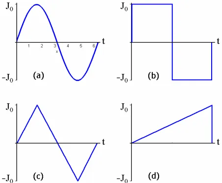
In order to produce the required heating pattern within a metal crucible and afterheater it is necessary to accu- rately model and predict the electromagnetic field and the eddy currents distribution produced by the RF-coil under different operating conditions such as geometry and orientation of the metallic parts, cross section of the coil turns, the crucible shape and position, and frequency choice [4-7]. Selection of input current shape is another critical issue, which is particularly important for certain selective heating applications. In this article, we try to investigate the effects of different input voltage shapes,

i.e., sine, square, triangle and sawtooth waveforms (

Fig-ure 1) on the strength and distribution of the electro-magnetic fields and heat generation in a Czochralski se-tup using the mathematical modeling and computer si-mulation. It should be noted, however, that despite of the differences in the patterns, each pattern is periodic. This point is important for our analysis of the driving current shape, i.e., they can be represented as closely as desired by the combination of a sufficiently large number of si-nusoidal patterns that form a harmonic series (Fourier series). Every non-sinusoidal current pattern consists of a fundamental and a complement of harmonics, which can be considered as a superposition of sine pattern of a fun-damental frequency ω and integer multiples of that fre-quency [8].

2. Mathematical Model

2.1. Governing Equations

Since the real induction heating process is very complex, we make some simplifying assumptions in our approach. In our mathematical model used for numerical calcula- tions, we make the following five assumptions: 1) the heating system is rotationally symmetric about the z-axis, so that all quantities are independent of the azimuthal coordinate φ; 2) all materials are isotropic, non-magnetic and have no net electric charge; 3) the displacement cur- rent is neglected; 4) the distribution of driving electrical current (also voltage) in the RF-coil is uniform; and 5)

[image:2.595.59.285.84.271.2]

Figure 1. Four input current shapes (a) Sine; (b) Square; (c) Triangle; and (d) Sawtooth waveforms of the induction coil.

the driving and induced currents have only one angular component (i.e., φ-direction). Under these assumptions, the governing equations are [4];

0

1 _B 1 _{B ˆ}

B J

r r r z r r 

  _{ }

 

  _   _{  }

   

         (1)

where

1 1

ˆ B

r r r z r r

B

 

 

    

 _{ } _

       

 _ (2)

and

coil coil coil

crucible

1

driving and eddy currents in the coil 1

eddy currents in the crucible

co B

d e d

cr B

e

J J J

r r t

J

J

r r t



 

 

  _{  }

 _

  

 _

  

 

(3) in which _B is the magnetic stream function defined by



, ,t



r



, , ,

B r z A r z t



  where Aφ is the azimuthal com-

ponent of the vector potential, the cylindrical coordinates, J the charge current density, σ the electrical conductivity, ₀



r z,



 the magnetic permeability of free space and t the time.

The energy dissipation rate in all metallic parts (coil, crucible and afterheater) is computed as



, ,



J2

P r z t 



 (4)

Finally we average over one period to obtain the vo-lumetric heat generation rate (i.e., the time averaged quantity),

 





2π

0

, P r, z,

2π

q r z   



where  is the frequency of the electrical current in the induction coil.

a) Sine Waveform

Assuming the driving current in the RF-coil as a sine form Jd J0sint, we can consider a solution of the form

 

 

sine _{, sin , cos}

B S r z wt C r z wt

   (6)

where S r z

 

, is the in-phase component and C r z

 

, is the out-of-phase component of the solution.

Now the coupled set of elliptic PDE’s for S r z

 

, and C r z

 

, is:

0 0 sine

0

coil

ˆ _crucible

0 elsewhere

co

co

J C

r

S C

r

_  _ 

  

 

   _

   

  

  

 (7)

0 sine

0

coil

ˆ _crucible

0 elsewhere

co

co S r

C S

r

         

  

  

 (8)

where ˆ is the linear operator defined in (2).

After solving (7) and (8) for S r z



,



and C r z

 

, , the eddy currents distribution and the energy dissipation rate can be computed via

 

 

sine _{, cos , sin}

cos sin (9)

B e

C S

J S r z wt C r z wt

r t r

J wt J wt



  

    _  _



 

and









2

2 2

2 0 0

2 2

2 2

2

sin coil

sin2 crucible (1 , ,

0)

co r r

co co

cr J

J J

S C S C

P r z t

t r

S C CS t

r 

  



   

  _



 _{   } 

 _  _  _  _ 

 

  

       

  

 

Consequently, the volumetric heat generation rate is

 





2 2

2 0

2 sine

2

2 2

2

coil ,

crucible

co r

co

cr

J

S C

r

q r z

S C

r

 

   

  _{ } 

       _   _  



 



b) Square Waveform

The square waveform of the driving current in the RF- coil can be approximated by a sum of harmoni

Fourier series as

cs using

 





square 0 0

1

sin 2 1 4

π 2 1

d

n

n t

J

J J F t

n       



(12)

and then

square square 1

B B n

n   



  _{ }







1

sin 2 1 cos 2

n n

n

S n t C n









_    1



t_

(13)  













square square 1 1 2 1

sin 2 1

cos 2 1

e e n n

n n

n n

J J C n

r S n         





 t

t_     (14)













0 square 2 1 4 coil 2 1 π

2 1 ˆ _crucible 0 elsewhere (15) co co n cr cr n _n n J C n r n S _C r              _               









square 2 1 coil 2 1 ˆ _crucible 0 elsewhere (16) co co n cr cr n n n S r n C S r                 

 

 













square square 1 2 2 2 2 0 2 2 1 2 2 2 2 2 1 , ,

2 1 4

coil

2 2 1 π

2 1 crucible (17) 2 n n co n n n _co cr n n n

q r z q r z

n J r

S C r n n S C r               _  _{ }    _{  }     _    _{   }    _  _{  }   







c) Triangle Waveform

The triangle waveform of the input current in the coi is approximated as

l

 

 









1 triangle 0

0 2 2

1

1 8

sin 2 1

π 2 1

n d

n

J

J J F t n t

n       



  (18)

t

 

1

B B n

n 









1

sin 2 1 cos 2 1

n n

n

S n t C n







_    _

triangle_



 triangle

    (19)  













triangle triangle 1 1 2 1

sin 2 1

cos 2 1

e e n

n n n n J J n C n r S n        _   





 t

t   (20)

 













1 0 2 2 triangle

1 8 2 1

coil 2 1 π

ˆ 2 1

crucible 0 elsewhere (21) n co co n cr cr n n J n C r n n S _C r         _{ }       _  _  _  _    









triangle 2 1 coil 2 1 ˆ _crucible 0 elsewhere co n c c r cr n o n n S r n C S r                

 ₍₂₂₎

 

 





 













triangle 2 2 2 1 1 0

triangle 2 2 3 2 1 2 2 1 2 2 2 , 2 1 2 1 8 coil 2 1 π

2 1 crucible 2 co n n n n n n _co n cr n n

q r z

n r

J r

q S C

n n S C r          _      _         _{ }              







      (23)

d) Sawtooth Waveform

The related equations of the sawtooth waveform of the input current can be written similar to the squ

triangle waveforms. They are

are and

 

sawtooth 0 0 2 1 sin π d n

J n t

J J F t

n 



  



 (24)

n

 





sawtooth sawtooth

B 



B n 



1 1

n n

sin cos

n

S n t C n t

 



    (25)

 





sawtooth sawtooth

1 1

sin cos

e e n

n n

n

n n

J J S n t C n t

r

 _{ }

 

 









 (26)

sawtooth

coil

ˆ _crucible

0 elsewhere

co co

n

cr cr

n n

n

S r n

C S

r

         

   

 (28)

 

 





sawtooth

2 2

2 0 2

2 2

1 sawtooth

2 2 1

2 2 2

1

,

coil

2 π

crucible 2

co

n n

n co

n n

cr

n n

n

q r z

n J r

S C

r n

q

n

S C

r 

 _

 



     

 

    

    

 _



 









 

   

(29)

2.2. The Calculation Conditions

The driving current density in the induction coil is calcu-lated by J₀_coV_coil



2πR N_coil



, where is total voltage of the coil, is the m

coil radius and N is the num of coil turns. e bound-ary conditions are

coil

V

ean value of the Th

the coil

R

ber 0

B

  ; both in the far field



r z,  



and at th metry (r

em for our

parameters

tem is shown in Figure und sing

s been method.

r distribution in the crucible, afterheater and R

e axis of sym = 0). ployed Values of electrical conductivity

calculations are presented in [9], operating

are listed in Table 1 and the geometry of the growth

heating sys 2. The f amental

partial equations require u a numerical discretization method to solve them. Calculation of the equations with boundary conditions ha made by 2D finite element

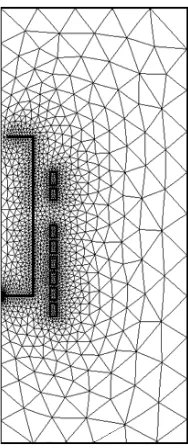
The two-dimensional computational domain with the finite element triangle mesh is shown in Figure3. In the space close to and in the metal parts (i.e. crucible, after-heater and RF-coil) the mesh is denser because of the high gradients of the electromagnetic fields. After solv- ing the set of equations, we can obtain the electromag- netic field structure in the system as well as the volumet- ric powe

[image:4.595.366.478.83.278.2]

F-coil.

Table 1. Operating parameters used for calculations.

Description (units) Symbol Value Crucible inner radius (mm)

Crucible wall thickness (mm) Crucible inner height (mm)

Baffle inner radius (mm) B

Heig

rc

lc

hc

rb

50 2 100

35 ottom heater height (mm)

ht of the thick bottom (mm) Coil width (mm) Coil wall thickness (mm)

D )

T Cur

hbh

htb

l

50 10 13 Radius of the round bottom corner (mm)

Coil inner radius (mm) rrcbco

10 78 Height of coil turns (mm)

istance between coil turns (mm otal voltage of the RF-coil (v) rent frequency of RF-coil (kHz)

co

lco

hco

dco

Vcoil

f

1.5 20 3 200

[image:4.595.62.291.87.253.2]

10

[image:4.595.376.470.308.532.2]

Figure 2. Sketch of an oxide Czochralski growth heating.

Figure 3. The finite element mesh structure of the calcula-tion domain.

3. Results and Discussion

We explain the results of electromagnetic field and heat- ing pattern in an oxide CZ setup including a cylindrical metal crucible, active afterheater and RF-coil correspond- ing to a real growth situation with different shapes of driv- ing current in the RF-coil and with unique amplitude and frequency.

3.1. Electromagnetic Fields

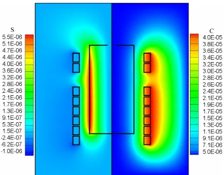
Figures 4-7 show the distribution of in-phase component and out-of-phase component of the magnetic stream function (ψB) for the cases of sine, square, triangle, and

[image:5.595.58.290.81.260.2]

Figure 4. Components of the magnetic stream function (ψB)

calculated for the case of sine waveform. The left hand side shows the in-phase component (S) and the right hand side shows the out-of-phase component (C) in the setup.

Figure 5. Components of the magnetic stream function (ψB)

calculated for the case of square waveform. The left hand side shows the in-phase component (S) and the right hand side shows the out-of-phase component (C) in the heating setup.

The maximum of in-phase component



Smax



while t

is located at the lowest and top edges of the RF-coil he mi- nimum



Smin



is located on the middle of the outer sur- face of crucible and afterheater wall, for the square and triangle waveforms. But for the sine and sawtooth wave-forms, it is vice versa, that is, the positions of the



Smax



and



C



are replaced. For the out-of-phase

compo-ent (C), the mimax

n nimum is located on th

f sine,

ase o

compo e outer surfaces of the induction coil turns for the cases o square and triangle waveforms while the maximum is placed there for the c f sawtooth waveform. The distribution of

[image:5.595.305.539.82.261.2]

C-component has a linear gradient in the space between the coil and the crucible and afterheater wall for all cases. The crucible and afterheater wall squeezes this -

Figure 6. Components of the magnetic stream function (ψB)

calculated for the case of triangle waveform. The left hand side shows the in-phase component (S) and the right hand side shows the out-of-phase component (C) in the heating setup.

Figure 7. Components of the magnetic stream function (ψB)

calculated for the case of sawtooth waveform. The left hand side shows the in-phase component (S) and the right hand side shows the out-of-phase component (C) in the heating setup.

nent to the area between the crucible and afterheater, and the RF-coil. Some interesting advantages are:

 The gradient of the S-component is too high in the

rly visible for all cases (edge effect). For the area close to the maximum and minimum points, which is not true for other parts of the system;

 Deformation and distortion of the S-component in the area close to the extreme edges of the RF-coil are particula

crucible and afterheater, spatial distribution of the S- component is along and parallel to their sidewall;

[image:5.595.57.289.315.490.2] [image:5.595.308.538.328.507.2]

3.2. Heat Generation

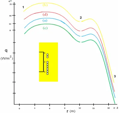
The volumetric heat generation rate (q) in the crucible and afterheater has been shown for all cases in Figure8. The power intensity is at its maximum value at the mid-dle portion of the outer surface of the crucible sidewall, which arises from the skin effect.

The most important features are:

 The heating structure of the crucible and afterheater is expect for their intensity. The is produced by square, sine, the same for all cases

most powerful energy

triangle and sawtooth waveform, respectively, Figure 9. This feature is predictable from the related elec-tromagnetic fields distribution;

[image:6.595.57.287.255.431.2]

(a) (b) (c) (d

Figure 8. Volumetric power distribution (q) in the crucib and afterheater computed for (a) sine; (b) square; (c) trian-gle; and (d) sawtooth waveform of the driving current (for a better demonstration the crucible and afterheater sidewal and bottom are separately magnified).

)

le

[image:6.595.308.539.332.557.2]

l

Figure 9. Profiles of the heat generated along the outer sur-face of the crucible and afterheater side wall calculated for (a) sine; (b) square; (c) triangle; and (d) sawtooth waveform of the input current.

 The spatial distribution of heat generation in the in-duction coil is mostly uniform with local “hot spots” (highly heated areas) at the lowest and upper edges, which is shown in Figure 10. The skin effect and pro- ximity effect are responsible for appearance of these undesirable overheating because the induced eddy cur- rents are concentrated on the top and lowest corners of the RF-coil [10,11];

 It is worth to note that despite of different total power generation, the coil efficiency (i.e., the part of the en-ergy delivered to the coil that is transferred to the workpiece) does not change and is approximately the same for all cases (Table 2).

4. Conclusions

erical calculations was performed. To study the dependence of electromagnetic distribution and heating pattern on the input current shape (sine, square, triangle and sawtooth waveforms) of the induction coil, a set of 2D num

(a) (b) (c) (d)

Figure 10. Volumetric power distribution (q) in the induc- tion coil calculated for (a) Sine; (b) Square; (c) Triangle; and (d) Sawtooth waveform of the input current.

Table 2. Detail information about the heat generated in the CZ coil (Heating efficiency is the part of the energy deliv-ered to the coil that is transferred to the crucible and after-heater).

Waveform _{afterheater (kW)}Crucible and Induction coil _{(kW) efficiency (%)} Heating

Sine 15 1.4 91.5

Square 26 2.4 91.6

Triangle 10 0.9 91.5

[image:6.595.74.273.501.689.2] [image:6.595.308.538.653.736.2]

From the computational results described above, we can conclude:

 The spatial structure of electromagnetic fields and generated heat is a complex function of several pa-rameters such as setup geometry and driving current shape;

 The electromagnetic fields distribution within the cru- cible and afterheater as well as the RF-coil is not uni-form. This electromagnetic fields nonuniformity causes a nonuniform heating pattern in the crucible and af-terheater, which in turn leads to a nonuniform tem-perature profile in the growth system.

A square input current results in a high intense heating of the crucible and afterheater while a sawtooth wave-form leads to a low heating intensity in that part of the system. Different amount of produced energy in the setu is due to differences in the intensity and distribution of the electromagnetic fields. Understanding the physics of

these

n-No. 3-4, 1989, pp. 792-826.

doi:10.1 (8

p

properties is important during designing of an i duction system for certain crystal growth applications.

REFERENCES

[1] J. J. Derby, L. J. Atherton and P. M. Gresho, “An Integra- ted Process Model for the Growth of Oxide Crystals by the Czochralski Method,” Journal of Crystal Growth, Vol. 97,

016/0022-0248 9)90583-6

[ Pulli the M

-lag, Berli eidelberg, 19 /978

2] D. T. J. Hurle, “Crystal ng from elt,” Springer

Ver n, H 93.

doi:10.1007 -3-642-78208-4 ent

[3] ein and Philip, “Transi Numerical

f Induc Heating dur Sublimation th of

O. Kl P. Investiga-

tion o tion ing Grow

Silicon Carbide Single Crystals,” Journal of Crystal Growth, Vol. 247, No. 1-2, 2003, pp. 219-235.

doi:10.1016/S0022-0248(02)01903-6

[4] M. H. Tavakoli, F. Samavat and M. Babaiepour, “Influen of Active Afterheater on the Induction Heating Process in ce Oxide Czochralski Systems,” Crystal Research and Tech- nology, Vol. 43, No. 2, 2008, pp. 145-151.

doi:10.1002/crat.200710993

[5] M. H. Tavakoli, A. Ojaghi, E. Mohammadi-Manesh and M. Mansour, “Influence of Coil Geometry on the Induc-tion Heating Process in Crystal Growth Systems,” Jour-nal of Crystal Growth, Vol. 311, No

1599.doi:10.1016/j.jcrysgro.2009.01.092. 6, 2009, pp. 1594- [6] M. H. Tavakoli, E. Mohammadi-Manes and A. Ojaghi, “In-

fluence of Crucible Geometry and P tion Heating Process in Crystal G

osition on the Induc- rowth Systems,” Jour- nal of Crystal Growth, Vol. 311, No. 17, 2009, pp. 4281- 4288.doi:10.1016/j.jcrysgro.2009.07.013

[7] M. H. Tavakoli, H. Karbaschi, F. Samavat and E. Moham- madi-Manesh, “Numerical Study of Induction

Melt Growth Systems—Frequency Selection,” Heating in Journal of Crystal Growth, Vol. 312, No. 21, 2010, pp. 3198-3203.

doi:10.1016/j.jcrysgro.2010.07.035

[8] G. H. Hardy and W. W. Rogosinski, “Fourier Series,” Do- ver, 1999.

[9] M. H. Tavakoli, “Modeling of Induction Heating in Oxide Czochralski Systems Advantages and Problems,” Crystal Growth Design, Vol. 8, No. 2, 2007, pp. 483-488.

doi:10.1021/cg070378+

[10] S. Zinn and S. L. Semiatin, “Elements of Induction Heat- ing,” ASM International, Cleveland, 1988.