Proceedings of the 57th Annual Meeting of the Association for Computational Linguistics, pages 457–470 457
Time-Out: Temporal Referencing for Robust Modeling of
Lexical Semantic Change
Haim Dubossarsky♠ Simon Hengchen♦ Nina Tahmasebi♣ Dominik Schlechtweg♥ ∗
♠Language Technology Lab, University of Cambridge ♦COMHIS, University of Helsinki
♣
Department of Swedish, University of Gothenburg ♥
Institute for Natural Language Processing, University of Stuttgart
[email protected] [email protected] [email protected] [email protected]
Abstract
State-of-the-art models of lexical semantic change detection suffer from noise stemming from vector space alignment. We have empiri-cally tested theTemporal Referencingmethod for lexical semantic change and show that, by avoiding alignment, it is less affected by this noise. We show that, trained on a diachronic corpus, the skip-gram with negative sampling architecture with temporal referencing outper-forms alignment models on a synthetic task as well as a manual testset. We introduce a prin-cipled way to simulate lexical semantic change and systematically control for possible biases.
1 Introduction
These past years have seen the rise of computa-tional methods to detect, track, qualify, and quan-tify how a word’s sense – or senses – change over time. These tasks are critical challenges that are relevant to a range of NLP fields, including the study of historical semantic change. The success-ful outcome of semantic change detection is rel-evant to any diachronic textual analysis, includ-ing machine translation or normalization of his-torical texts (Tjong Kim Sang et al.,2017), the de-tection of cultural semantic shifts (Kutuzov et al.,
2017) or applications in digital humanities ( Tah-masebi and Risse,2017a). However, currently, the best-performing models (Hamilton et al., 2016b;
Kulkarni et al., 2015; Schlechtweg et al., 2019) require a complex alignment procedure and have been shown to suffer from biases (Dubossarsky et al.,2017). This exposes them to various sources of noise influencing their predictions; a fact which has long gone unnoticed because of the lack of standard evaluation procedures in the field.
We examine the modeling approach of Tempo-ral Referencing(TR) which avoids post hoc
align-∗
The order has been randomly determined and all authors contributed equally to this work.
ment and is applicable to any vector space learning technique. We show that it (i) is less affected by noise and (ii) clearly outperforms state-of-the-art alignment models on a synthetic change detection task. The task is based on data from a synchronic corpus into which we artificially inject lexical se-mantic change (LSC) in a controlled and semanti-cally principled way. We further evaluate the mod-els on a manual testset of diachronic LSC and ex-amine their properties.
In this paper, we focus on skip-gram with neg-ative sampling (SGNS) models (Mikolov et al.,
2013) and PPMI (Levy et al.,2015) and make use of TR to share context information across time pe-riods, while learning individual embeddings for a target word in each time period. We evaluate mod-els in two ways: on the one hand, through the com-parison of model performance between semanti-cally changing and stable words. This is achieved through the synthetic introduction (and removal) of polysemy, mimickingSch¨utze(1998);Kulkarni et al.(2015);Rosenfeld and Erk(2018). We differ from previous work by creating those changes in a more structured way, and for many time points. The second type of evaluation put forward is a study built on a smaller number of words manu-ally classified as changed or stable.
Our contributions are the following:
• Noise Reduction: We avoid post hoc align-ment by TR and show that it outperforms other models and is robust to noise.
• LSC Simulation: We propose a systematic and principled method of injecting semantic change in a controlled fashion.
• Evaluation: We evaluate (i) by testing for noise reduction in a control condition, (ii) on large and controlled artificial data and (iii) on a manually annotated LSC testset.
frame-work to test any model of semantic change for their levels of noise and sensitivity in de-tecting simulated semantic change.
2 Related Work
Models of LSC Detection Computational ap-proaches to semantic change detection can be di-vided in different families: count-based semantic spaces (Sagi et al., 2009;Gulordava and Baroni,
2011) and more recently based on neural embed-dings (Kim et al.,2014;Basile et al.,2016; Kulka-rni et al., 2015; Hamilton et al., 2016b); graph-based models (Tahmasebi and Risse,2017a;Mitra et al., 2014, 2015); and finally topic-based (Lau et al.,2012;Wang et al.,2015;Frermann and La-pata,2016;Hengchen,2017;Perrone et al.,2019). Recently, we have seen dynamic embeddings with the main aim to circumvent alignment, and share data across time points, thus reducing data volume requirements. Using different base embeddings, SGNS (Bamler and Mandt, 2017), PPMI (Yao et al.,2018), and Bernoulli embeddings (Rudolph and Blei,2018), the results show that sharing data is beneficial regardless of the method.1 Tempo-ral Referencing has been applied first in the field of term extraction Ferrari et al. (2017) and re-cently been tested for diachronic LSC detection (Schlechtweg et al.,2019).
Evaluation Due to a lack of proper evalua-tion methods and datasets, all papers above have performed different, non-comparable evaluations. Previous evaluation procedures mainly tackle a few words: case studies of individual words ( Wi-jaya and Yeniterzi, 2011; Jatowt and Duh, 2014;
Hamilton et al.,2016a), or a comparison between a few changing and semantically stable words (Lau et al., 2012; Schlechtweg et al., 2017). Other works focus on the post hoc evaluation of their re-spective models (Kulkarni et al., 2015;Eger and Mehler, 2016). Importantly, Dubossarsky et al.
(2017) proposed to use a control condition to mit-igate the absent of validated evaluation methods and datasets.
Control Condition Evaluating empirical results often demands comparing these under a control condition in order to maintain that these are indeed
1For an extensive survey of computational approaches to
lexical semantic change, we refer the readers toTahmasebi et al.(2018), and toKutuzov et al.(2018) for a specialized focus on diachronic word embeddings.
valid and are not the result of unwanted confound-ing factors. A control condition directly follows from a specific research hypothesis, and therefore must resemble the original condition in any as-pect, except the variable of interest that is being hypothesized about. For example, Dubossarsky et al.(2017) attested that a shuffled diachronic cor-pus is a proper control condition to test models for semantic change, under the hypothesis that such models indeed capture semantic change and not something else. They concluded that any degree of semantic change that is reported by a model on the shuffled corpus may only be related to noise, instead of a true semantic change. Similarly, we propose to test the noise levels associated with dif-ferent semantic change models using a shuffled historical corpus, and evaluate their true degree of semantic change by comparing their results to the original historical corpus. Importantly, there are many ways to create control conditions, and the synthetic lexical semantic change proposed in Section4 contains another type of control condi-tion, that is based on artificially induced semantic change.
3 Models
Embeddings A common method in LSC detec-tion is to learn low-dimensional semantic vec-tor spaces (embeddings) for specific time periods and then align spaces for consecutive time periods with an orthogonal mapping which minimizes the distances between the time-specific vectors for all words (Hamilton et al.,2016b). Given two consec-utive time periodsa,b, and corresponding text cor-poraCa,Cb, we learn two vector spacesA,B.
Or-thogonal Procrustes analysis can then be applied to find the optimal mapping matrixW∗ such that the sum of squared Euclidean distances betweenB’s mappingBW andAis minimized:
W∗= arg min
W kBW −Ak
2.
The optimal solution for this problem is given by an application of Singular Value Decomposition (Artetxe et al., 2017).2 The degree of LSC of a wordwis then measured with the cosine distance (Salton and McGill, 1983) between w’s vectors in A and BW∗ (B’s mapping). This approach
2W is constrained to be orthogonal. Aand B are first
has been found to outperform other LSC detec-tion methods in various studies (Hamilton et al.,
2016b; Kulkarni et al., 2015). It has the advan-tage of not assuming that words keep the same meaning over time. A presumable downside of this approach is expected noise from the align-ment, i.e., it may not be possible to align all words to each other that have similar meanings, because the spaces were learned independently.
PPMI Another method to learn time-specific se-mantic vector space representations A, B is to store count-based co-occurrence information for each word in a high-dimensional sparse matrix and then apply Positive Pointwise Mutual Information (PPMI) weighting (Levy et al., 2015). In such a matrix each column stores the co-occurrence statistics with a specific context word. This has the advantage that A and B can be aligned straight-forwardly, because many context words occur as columns in both A and B and can hence be mapped onto each other. MappingA andB to a common coordinate axis then corresponds to in-tersecting their columns (Hamilton et al.,2016b). This has the advantage of avoiding the complex alignment procedure for embeddings, but also loses their performance advantages (Baroni et al.,
2014;Levy et al.,2015).
Temporal Referencing Temporal Referencing (TR) is an alternative to learning individual word representations for different time periods, which avoids alignment using a procedure radically sim-pler than proposed for dynamic embeddings. TR is potentially applicable to every vector space learning method. We treat all time-specific cor-pora Ca, Cb, ..., Cn as one corpus C and learn
word representations on the full corpus. However, we first replace each target wordw ∈ Ct with a
time-specific token wt.3 This temporal
referenc-ing ofwis only performed when it is a target word, when the word is considered a context word, it re-mains unchanged. Following this procedure, we learn one single space that contains a vector for each target-time pairwt, which may be compared
directly without the need for alignment. Besides the considerable advantages of avoiding alignment and being applicable to count-based and embed-ding methods, it presumably lowers data require-ments (because context words are collapsed, and
3In our case, t is a decade. E.g., in the corpus for
1920 we replace each occurrence ofcomputerwith the string
computer1920.
thus shared, across corpora). Accordingly, we as-sume TR to produce smoother change values. As various other models, TR relies on the assumption that the semantics of the context words stays rela-tively stable over time.
4 Synthetic Lexical Semantic Change
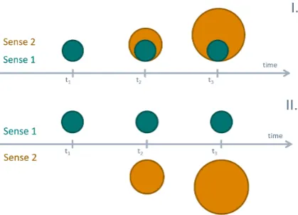
We aim to simulate semantic change under con-trolled settings, while keeping the corpus as natu-ral as possible.4 We call this proceduresense in-jection. We increase the semantic material of a recipient wordwrin subsequent subcorpora by in-jecting contexts from a donor wordwd. The
con-text of the recipient word (illustrated as Sense 1 in Figure1) stays as it is in the corpus. The first subcorpus contains only contexts from the recip-ientwr and all the contexts of the donor wd are removed. In the next time period we add 25% of the contexts ofwd, with donor word replaced by the recipient word. In each subsequent corpus, an additional 25% of the donor word are injected un-til the last time periods contain equal amounts of contexts from the donor and recipient. As a result, seen from the recipient wr, the last time periods have double the amount of contexts as in the first time period|wr(t
n) +wd(tn)|= 2∗ |wr(t1)|. Note that due to the polysemous nature of words (each is usually associated with more than one sense), we preferred toaddthe donor words’ con-texts instead of simplyreplacingthe existing con-texts of the recipient words with the concon-texts of the donor words. This is because the former involves a single source of synthetic lexical semantic change, while the latter involves two sources (the removal of contexts associated with different senses of a recipient word, as well as the added contexts as-sociated with the senses of a donor word). As a result, this procedure yields less noisy examples of synthetic lexical semantic change.
We differ between cases where recipient and donor are related (e.g. maker→creator, Fig.1a) and unrelated (e.g. shoulders →horde, Fig. 1b), following e.g.,Pilehvar and Navigli(2013). This procedure is aimed to give us insight into how much novel semantic material is needed for our methods to detect semantic change. Our hypothe-sis is that cases where the donor word is unrelated to the recipient word should be simpler to detect compared to those that are in close relation. It is
4Hence, the target words’ frequencies were not matched,
Figure 1: Increase in semantic material for a word by means of sense injection. I.: new injected sense is re-lated to the existing sense. II.: new injected sense is unrelated.
linguistically motivated to choose semantically re-lated words to simulate sense change; those are the most difficult cases of sense change, and a likely procedure of semantic change introducing poly-semy (Blank,1997).
Finally, to simulate the same increase in fre-quency, we repeat the sense injection for a set of control words. In this case recipient and donor word are the same wr = wd. This creates the same increased frequency of the recipient word
|wr(t
n)| = 2 ∗ |wr(t1)| as the above, but with-out any added semantic information because the control word keeps its original contexts.
5 Experimental setup
5.1 Corpora
For Experiment 1 (Sec. 6.1) we used COHA (Davies,2002), of which we restrict ourselves to decadal bins spanning from 1920 to 1970 so as to have a comparable number of tokens for each time slice. For Experiment 2 (Sec.6.2) we used COCA (Davies, 2008), of which we remove the spoken and academic genres in order to maintain a more similar usage context of words. As a control set-ting, we created shuffled versions of the same cor-pora with the same periods, and straightforwardly followedDubossarsky et al.(2017).
5.2 Synthetic semantic change
For related words, we used the Noun-Noun pairs in SimLex-999 (Hill et al., 2015) as a starting point. However, even semantically unrelated pairs in SimLex were deemed somewhat related by our annotators, and therefore we kept only 10 of those.
We created the rest of the list of unrelated words as follows: we randomly sampled 300 lowercased nouns5from our corpus, which we assembled into 150 pairs. We then asked three annotators to in-dependently go through the list of generated pairs and determine whether they were semantically re-lated or not. All 150 pairs were deemed seman-tically unrelated by at least 2 annotators. Only 5 pairs had a disagreement but were qualified as border line cases by the disagreeing annotator, and kept. This procedure yielded 356 word pairs in to-tal, of which 196 were related and 160 were not related.
5.3 Model training
We tested two models in our experiments: (i) low-dimensional embeddings learned with SGNS and (ii) high-dimensional sparse PPMI vectors. Each of these were tested with their respective align-ment method (AL) and with Temporal Referenc-ing (TR) as described in Section3, leaving us with four models to compare:
SGNSAL SGNSTR
PPMIAL PPMITR
In order to avoid that replaced target words co-occur with other target words in TR we used the implementation of Levy et al. (2015), allowing us to train SGNS and PPMI on extracted word-context pairs instead of the corpus directly. For this, we iterated over corpus Ct such that for
each token w and for each of its context words
c within a symmetric window we extracted the word-context pair: (wt,c) ifwis a target word and
(w,c) otherwise.
In this way, we guarantee a target word is never replaced and treated as context of any other word. For TR, SGNS and PPMI were then trained on these extracted pairs. For AL, we extracted only regular word-context pairs (w,c) and trained SGNS and PPMI on these. LSC is measured for all four models via cosine distance.6 (See Appendix
Afor preprocessing and hyper-parameter details.)
6 Evaluation
To test our methods we performed three main experiments, comparing the performances of TR to the existing state-of-the-art diachronic model
5
The filtering was carried out on the basis of the output of NLTK (Bird et al.,2009)’spos tag()function.
6Find a full implementation of the pipeline athttps://
alignment. In the first experiment, we compare the models’ performance under control conditions that address complementary (potential) weaknesses. The second experiment tests different synthetic change types and assesses whether better models improve detection of lexical semantic change, in a controlled setting. Finally, we test our methods on a manually created testset on a genuine corpus, and manually inspect the results.
6.1 Experiment 1: Model comparison
In this experiment, we trained each model on two corpora, one genuine diachronic corpus with nat-ural semantic change, and one shuffled where the diachronic change is distributed equally across all time periods (see Sec. 5.1). We study the average change of cosine distance as a proxy for semantic change. FollowingDubossarsky et al.(2017) we consider the average cosine distance (acd) trained on the genuine corpus to correspond to true se-mantic change + noise. In contrast, the average co-sine distance on the shuffled corpus corresponds to pure noise. Therefore, the difference between the two equals to true signal, or in other words, true lexical semantic change.
Importantly, we are interested in investigating, and hopefully mitigating, possible sources of the noise that might be found in some of the mod-els. Specifically, we hypothesize that the align-ment procedure adds considerable noise to the acd, and plan to test how TR can alleviate some of that noise. Moreover, TR is assumed to con-tribute not only by circumventing the alignment, but also by producing more stable context vectors due to the increased amount of data on which they are trained.7 Therefore, we first tease-apart these factors using the following comparisons between the different models.
1. For all models, we consider the difference in average cosine distance between gen-uine and shuffled conditions (acdgenuine −
acdshuf f led) as being inversely proportional
to the amount of noise that the original model unknowingly captures. Hence, the larger the difference, the less noisier (and better) the model is. We consider this to be an approxi-mation of thetrue semantic change.
7
We differ between stable vectors that do not change despite the randomness involved in training between multi-ple runs, andaccuratevectors give a good representation of meaning. Note that when we use the termstable word we mean stable in meaning over time.
2. Focusing on the differences between the two PPMI models allows us to test the indepen-dent contribution of TR in providing more accurate context vectors because the inter-section of the PPMI vectors are inherently aligned.
3. Focusing on the SGNS models conflates the potential benefits from more accurate context vectors with the disadvantage of Procrustes alignment (which is necessary for SGNSAL but not for SGNSTR).
4. The difference between the last two would al-low us to evaluate the independent contribu-tion of these two sources on the (presumably) less noisy SGNSTRmodel scores.
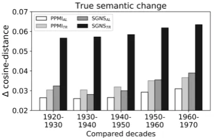
[image:5.595.312.521.394.529.2]Results (experiment 1) We start analyzing the true semantic change for each of the models (PPMIAL to PPMITR and SGNSAL to SGNSTR) over the corpus. In Figure2, we can see that tem-poral referencing introduces less noise throughout the 5 decadal comparisons. For both PPMI and SGNS, the true semantic change increases for the TR models compared to the aligned.
Figure 2: Comparison of aligned embedding spaces and temporal referencing using both the genuine and the shuffled corpora. High difference in cosine distance indicate less noise captured by the model.
factors that improve prior models; firstly, it avoids the need for alignment altogether (and the noise that usually comes with it), and secondly, it pro-duces more stable context vectors due to the in-creased volume of data when using the full corpus.
Table 1: Difference in average cosine distance between genuine and shuffled conditions (true semantic change) for each method, collapsed over the 5 time bins (1920– 1970) in COHA.
Align TR ∆
SGNS 0.033 0.059 0.026
PPMI 0.028 0.033 0.005
Smoothness of Temporal Referencing We fur-ther analyzed the nature of the progression of the cumulative semantic change that words ex-hibit over time. Under the assumption that words change their meaning in a systematic way, it fol-lows that words’ semantic change would increase over the years. Therefore, an ecologically valid model of semantic change should show that the words change more as the time interval for com-parison increases, for the vocabulary as a whole. In contrast, if a model captures stochastic fluctua-tions in the words’ vectors instead of true semantic change, then such a shift in the distribution will be less prominent.
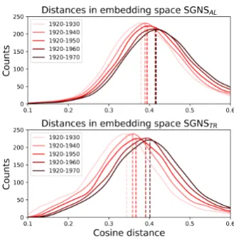
We plot the distribution of the words’ cosine distances with increasing time intervals (relative to 1920) for both SGNS models in Figure 3. Both models show a gradual transition from left (smaller change scores) to right (larger change scores). This corroborates our basic assumption that words change more as the time interval for comparison increases. Crucially, Temporal Refer-encing shows a more constant cumulative progres-sion of cosine distances over time in contrast to alignment where decadal cosine distance distribu-tions seem to be more volatile. We followBamler and Mandt(2017) in interpreting these results as attesting for the relatively high noise factor in the SGNSALover the SGNSTR.
Overall, the different analyses converge to the same conclusion: Temporal Referencing is a bet-ter model for capturing a word’s semantic infor-mation from diachronic text because it introduces less noise. Next, we will investigate if a less noisy model is also better at detecting semantic change.
Figure 3: Smoothed histograms of word distances for the two SGNS models. For the TR model, we see a more constant cumulative shift which is reflected by the overlap between the distributions as well as by dif-ferences in their means (dashed vertical lines).
6.2 Experiment 2: Synthetic semantic change
This experiment aims to see how well our meth-ods can find different synthetic change types. In order to minimize natural semantic change in the dataset, we made use of the synchronic dataset COCA which we randomly shuffled, and simu-lated a diachronic corpus for which we have 7 time-bins. We randomly assigned a seventh of COCA to each of our artificial time periods, la-beled t1 to t7. Sentences in which either word of the synthetic semantic change pairs (see Sec.
4) or their corresponding control words appeared were held out. These sentences were subsequently added back to COCA according to the procedure outlined in Section 4, which enabled us to con-trol for the fixed ratio incremental steps between the recipient and donor words (i.e., changes to the injection ratio were made only fort2-t3,t3-t4,t4
-t5, and t5-t6, while t1-t2 and t6-t7 had no such changes).
All four models were trained on the 7 synthetic time-bins exactly as in Experiment 1. The tar-get words were the 356 words with synthetic lexi-cal semantic change and their 356 control words that were matched with the same frequency in-crease but otherwise are considered semantically stable. For each target word, the cosine distances between two consecutive synthetic time-bins were computed, resulting in 6 change scores per word.
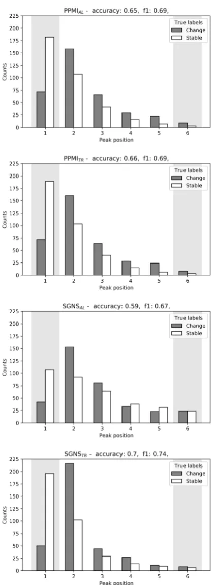
it shows the maximum cosine distance). In order to evaluate the models’ ability to truly detect se-mantic change, we formulate a na¨ıve binary clas-sification task based on the words’ peak positions. For each word, if the peak is in position 2–5, we classify it as changed, and otherwise as stable and measure accuracy and F1-score.
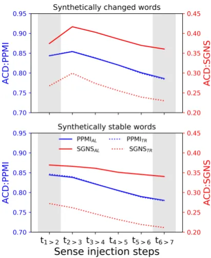
[image:7.595.310.525.358.436.2]Results Figure4shows theacdof the four mod-els for the change and stable words separately, ac-cording to the different sense injection ratios. The two plots differ markedly. For the semantic change words (upper plot), all four models show a notice-able peak when the new sense was first injected (step 2), followed by a steady decrease inacduntil step 6. In contrast, the stable words only show the steady decrease starting from step 1, without any noticeable peaks. This decrease probably stems from the target words’ increased frequency that can lead to more accurate word embeddings ( Hell-rich and Hahn,2016). Because peaks in acdare interpreted as points were semantic change was the most profound, the results support the models’ ability to detect synthetic semantic changes.
Figure 4: acdat different sense injection steps for the four models. Steps without sense injection are shaded.
Although the majority of peaks for the semantic change words fall in step 2, as expected by theacd analysis above, words had their peaks in other step
positions as well (see AppendixB).8
Table 2 reports accuracy and F-scores for the four models in the binary classification task. As clearly seen, all four models perform better than chance even under these very rudimentary condi-tions (finding the argmax of a vector of length 6). Crucially, SGNSTR outperforms the rest of the models, and especially SGNSALthat shows the worst performance. These results corroborate our hypothesis from Experiment 1 that noise is neg-atively influencing task performance. By allevi-ating the noise factor that exists in SGNSAL(due to alignment), SGNSTRis able to show substantial gains in this binary classification task.
Table 2: Accuracy (averaged, and split into individual classes) and F1-scores for semantic change detection. For stable words (control words), peaks at 1 and 6 steps are correct. For change words, peaks at steps 2–5 are correct. We see that all methods find unrelated change better than related change, and that SGNSTR outper-forms the other methods.
PPMIAL PPMITR SGNSAL SGNSTR
Stable 0.52 0.54 0.37 0.57
Unrelated 0.83 0.83 0.86 0.91
Related 0.73 0.73 0.78 0.78
Mean acc. 0.65 0.66 0.59 0.70
F1-score 0.69 0.69 0.67 0.74
Discussion Table 2 shows that SGNSTR gains its performance advantage over SGNSAL mainly from a better classification of the stable words (0.37 vs. 0.57). In order to understand this bet-ter, we inspect their mean cosine distance curves only for stable words in Figure5. SGNSTR’s curve clearly declines, while SGNSAL’s curve declines much less and is more volatile. We attribute the decline of both curves to the diminishing noise that comes from the continuous increase in frequency of the control words (Dubossarsky et al., 2017). It seems that this diminishing frequency noise is counteracted by the alignment noise, yielding a flatter curve for SGNSAL. The latter increases SGNSAL’s chance to have peaks in one of the center injection steps producing false positives in our classification task. However, this property may also have a positive influence on SGNSAL in related LSC detection tasks (Schlechtweg et al.,
2019).
8We also ran experiments with moving the time point
[image:7.595.77.283.405.657.2]Figure 5: Mean cosine distance curves for SGNSTR and SGNSAL.
6.3 Experiment 3: WSC testset
So far, the results have been based on either a large random sample to show general tendencies for the language in the corpus as a whole, or syntheti-cally injected semantic change. In this part, we test the behavior of our methods on a small, man-ually created testset for semantic change. We use the Word Sense Change Testset (Tahmasebi and Risse, 2017b) that consists of words and the dif-ferent associated change events, for the time span 1785 – 2010. In this experiment, we ignore the sense changes and consider only words as changed or stable, and restrict our change words to those that have change events between 1920 and 1970.9 In total we have 13 changed and 19 stable words (excluding words with a total frequency≤100).
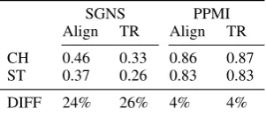
Table 3:acdfor WSC testset. Var∈(0.0−0.01). CH = changed word, ST = stable word, DIFF = difference between ACD for change and stable in percent.
SGNS PPMI
Align TR Align TR
CH 0.47 0.31 0.86 0.86 ST 0.34 0.21 0.71 0.73
DIFF 38% 50% 20% 17%
In Table 3 we see acd of each model on the changed and stable words. We find that for all methods, SGNSAL, SGNSTR, PPMIAL and PPMITR, theacdfor the changed words is statis-tically significantly higher (p values≤0.01) than for the stable words which nicely corresponds to intuition; words with true semantic change should have vectors that differ more than words without change. The mean difference between the stable and the changed words, that gives us some notion
9As an example, the word
[image:8.595.80.283.66.185.2]caris considered stable since its change event occurred before 1920.
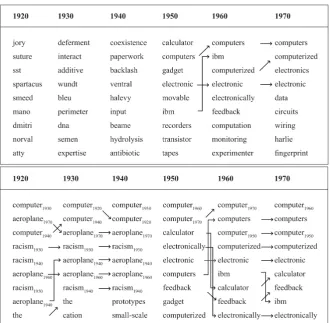
Figure 6: Nearest neighbors forcomputer. Upper part SGNSAL, lower part SGNSTR. A larger rendering of this figure is available in AppendixD.
of how well the two different classes are separated, is highest for SGNSTR. Because of the limited size of the testset, the results are indicative rather than conclusive and we continue with a manual analy-sis of the nearest neighboring words.
We carry out a qualitative evaluation for the closest neighbors for computer (see Figure 6), a word we expect to have changed after the inven-tion of the digital computer in the 1940s, for the SGNS aligned version and SGNS with Temporal Referencing. SGNSAL has only a few words in common in 1950–1970, and while the digital com-puter is showing here, there are few overlapping words. The time periods 1920–1940 have no com-mon words. In comparison, the SGNSTR show clear patterns. We see a clear break between 1940 and 1950, without any overlapping word, and a pattern between 1950–1970; the closest words are the othercomputer1940–1970.10 This is exactly the pattern that we expected to see using the sense in-jection; stable senses can be distinguished from changing senses by their relationship to the other temporally referenced vectors.
Next, we study a word for which we expect no sense change, namely ship (see Appendix E). The SGNSALshow a fairly lowacd, but still there
10
The closest words in 1920–1940 have high cosine dis-tances and are thus not very related. Still, for each
computertime, the other vectors ofcomputerare among the
[image:8.595.104.258.523.589.2]Table 4:acdfor synthetic change. Var∈(0.0−0.01).
SGNS PPMI
Align TR Align TR
CH 0.46 0.33 0.86 0.87 ST 0.37 0.26 0.83 0.83
DIFF 24% 26% 4% 4%
are large differences in the top neighboring words. The SGNSTRshow what we expect; the most simi-lar words are the othership1920–1970, and over time we see that the ‘self-similarity’ decreases. For al-most all decades, the al-most similar words areship from the decade before and after. The lower words also help describe the meaning ofship, as aboat and later also as aspaceship. The pattern of stabil-ity is much more clear for SGNSTRthan SGNSAL and holds for most other stable words as well.
For the word tape, that has a change in domi-nant sense (or an addition of another strong sense) with the addition of the music tape to adhesive tape, we see the same patterns as for ship, but the bottom words containribbon, paper, adhesive for 1920–1940 and recorder, recording, stereoin 1950–1970.11
For both the real change in Table3and the syn-thetic change in Table4, we find that SGNSTR is best at differentiating between the stable and the change classes for both datasets (50% for WSC and 26% for synthetic change).
7 Conclusions and future work
In this paper, we have empirically tested the temporal referencing method for lexical seman-tic change. We train one vector space model over the whole corpus, and thus share informa-tion of the context words while training individ-ual vectors for each target word and time period. We compare two commonly used models, namely PPMI and SGNS because of their properties; the PPMI model is count-based and does not require alignment across time, while the SGNS model has shown state-of-the-art results in previous work.
We find that the SGNS model trained with Tem-poral Referencing contains significantly less noise than the standard SGNS for which an alignment is necessary. In comparison, for the PPMI model where no alignment is needed, Temporal
Refer-11Find all nearest neighbour lists athttps://github.
com/Garrafao/TemporalReferencing/tree/ master/data.
encing also significantly reduced the noise level, but to a lesser extent.
Next we evaluated whether the noise reduction carries over performance on a synthetic lexical semantic change detection task. We simulated change in a controlled and semantically principled way, using sense injection and showed that words with semantically related and unrelated semantic change can be differentiated from control (stable) words that are not sense injected, but increase in frequency in the same way as the changed words. SGNS with Temporal Referencing outper-forms the other methods in correctly classifying the words to the two classes (change vs. stable).
Finally, we evaluated on a small, handcrafted set of change and stable words and found that SGNS with Temporal Referencing gives the largest separation between words that undergo se-mantic change and those that stay stable over time. In particular, we observe a similar behavior be-tween this smaller testset and the synthetic sense injection, supporting our sense injection method as a good proxy for isolating and studying lexical semantic change.
Our results support the following conclusion; trained on a diachronic corpus, SGNS with Tem-poral Referencing will capture more true semantic change.In the future, we plan to evaluate Tempo-ral Referencing against the related dynamic em-bedding models on an annotated empirical lexi-cal change dataset with multiple languages. We also plan on testing how well Temporal Refer-encing deals with corpora that are too small for alignment-based methods, hopefully opening new avenues of quantitative research.
Acknowledgements
References
Mikel Artetxe, Gorka Labaka, and Eneko Agirre. 2017. Learning bilingual word embeddings with (almost) no bilingual data. InProceedings of the 55th Annual Meeting of the Association for Computational Lin-guistics (Volume 1: Long Papers), pages 451–462.
Robert Bamler and Stephan Mandt. 2017. Dynamic word embeddings. InProceedings of the 34th In-ternational Conference on Machine Learning, vol-ume 70, pages 380–389.
Marco Baroni, Georgiana Dinu, and Germ´an Kruszewski. 2014. Don’t count, predict! A systematic comparison of context-counting vs. context-predicting semantic vectors. 52nd Annual Meeting of the Association for Computational Lin-guistics, ACL 2014 - Proceedings of the Conference, 1:238–247.
Pierpaolo Basile, Annalina Caputo, Roberta Luisi, and Giovanni Semeraro. 2016. Diachronic analysis of the Italian language exploiting Google Ngram. In
Third Italian Conference on computational Linguis-tics CLiC-it 2016.
Steven Bird, Ewan Klein, and Edward Loper. 2009.
Natural language processing with Python: analyz-ing text with the natural language toolkit. O’Reilly Media, Inc.
Andreas Blank. 1997. Prinzipien des lexikalischen Bedeutungswandels am Beispiel der romanischen Sprachen. Niemeyer, T¨ubingen.
Mark Davies. 2002. The Corpus of Historical Amer-ican English (COHA): 400 million words, 1810-2009. Brigham Young University.
Mark Davies. 2008. The corpus of contemporary American English (COCA): 400+ million words, 1990-present. Brigham Young University.
Haim Dubossarsky, Daphna Weinshall, and Eitan Grossman. 2017. Outta control: Laws of semantic change and inherent biases in word representation models. InEMNLP 2017, pages 1136–1145. ACL.
Steffen Eger and Alexander Mehler. 2016. On the lin-earity of semantic change: Investigating meaning variation via dynamic graph models. InACL 2016, pages 52–58. ACL.
Alessio Ferrari, Beatrice Donati, and Stefania Gnesi. 2017. Detecting domain-specific ambiguities: an NLP approach based on wikipedia crawling and word embeddings. In2017 IEEE 25th International Requirements Engineering Conference Workshops (REW), pages 393–399. IEEE.
Lev Finkelstein, Evgeniy Gabrilovich, Yossi Matias, Ehud Rivlin, Zach Solan, Gadi Wolfman, and Eytan Ruppin. 2001. Placing search in context: The con-cept revisited. InProceedings of the 10th Interna-tional Conference on World Wide Web, WWW ’01, pages 406–414, New York, NY, USA. ACM.
Lea Frermann and Mirella Lapata. 2016. A Bayesian model of diachronic meaning change. TACL, 4:31– 45.
Kristina Gulordava and Marco Baroni. 2011. A distri-butional similarity approach to the detection of se-mantic change in the Google Books Ngram corpus. InGEMS 2011, pages 67–71. ACL.
William L. Hamilton, Kevin Clark, Jure Leskovec, and Dan Jurafsky. 2016a. Inducing domain-specific sen-timent lexicons from unlabeled corpora. InEMNLP 2016, pages 595–605. ACL.
William L. Hamilton, Jure Leskovec, and Dan Jurafsky. 2016b. Diachronic word embeddings reveal statisti-cal laws of semantic change. InACL 2016, pages 1489–1501. ACL.
Johannes Hellrich and Udo Hahn. 2016. Bad com-pany—neighborhoods in neural embedding spaces considered harmful. In Proceedings of COLING 2016, the 26th International Conference on Compu-tational Linguistics: Technical Papers, pages 2785– 2796.
Simon Hengchen. 2017. When Does it Mean?: De-tecting Semantic Change in Historical Texts. Ph.D. thesis, Universit´e libre de Bruxelles.
Felix Hill, Roi Reichart, and Anna Korhonen. 2015. Simlex-999: Evaluating semantic models with (gen-uine) similarity estimation. Computational Linguis-tics, 41(4):665–695.
Adam Jatowt and Kevin Duh. 2014. A framework for analyzing semantic change of words across time. In Proceedings of Joint Conference on Digital Li-braries, JCDL ’14, pages 229–238.
Yoon Kim, Yi-I Chiu, Kentaro Hanaki, Darshan Hegde, and Slav Petrov. 2014. Temporal analysis of lan-guage through neural lanlan-guage models. In Proceed-ings of the ACL 2014 Workshop on Language Tech-nologies and Computational Social Science LACSS 2014, pages 61–65. ACL.
Vivek Kulkarni, Rami Al-Rfou, Bryan Perozzi, and Steven Skiena. 2015. Statistically significant de-tection of linguistic change. InProceedings of the 24th International Conference on World Wide Web, WWW ’15, pages 625–635.
Andrey Kutuzov, Lilja Øvrelid, Terrence Szymanski, and Erik Velldal. 2018. Diachronic word embed-dings and semantic shifts: A survey. InProceedings of COLING 2018, pages 1384–1397, Santa Fe. ACL.
Jey Han Lau, Paul Cook, Diana McCarthy, David New-man, and Timothy Baldwin. 2012. Word sense in-duction for novel sense detection. InEACL 2012, pages 591–601.
Omer Levy, Yoav Goldberg, and Ido Dagan. 2015. Im-proving distributional similarity with lessons learned from word embeddings. Transactions of the Associ-ation for ComputAssoci-ational Linguistics, 3:211–225.
Tomas Mikolov, Ilya Sutskever, Kai Chen, Greg Cor-rado, and Jeffrey Dean. 2013. Distributed represen-tations of words and phrases and their composition-ality. InProceedings of NIPS.
Sunny Mitra, Ritwik Mitra, Suman Kalyan Maity, Martin Riedl, Chris Biemann, Pawan Goyal, and Animesh Mukherjee. 2015. An automatic ap-proach to identify word sense changes in text media across timescales. Natural Language Engineering, 21(5):773–798.
Sunny Mitra, Ritwik Mitra, Martin Riedl, Chris Bie-mann, Animesh Mukherjee, and Pawan Goyal. 2014. That’s sick dude!: Automatic identification of word sense change across different timescales. In
ACL 2014, pages 1020–1029.
Valerio Perrone, Marco Palma, Simon Hengchen, Alessandro Vatri, Jim Q. Smith, and Barbara McGillivray. 2019. GASC: Genre-aware semantic change for Ancient Greek.CoRR, abs/1903.05587.
Mohammad Taher Pilehvar and Roberto Navigli. 2013. Paving the way to a large-scale pseudosense-annotated dataset. InProceedings of the 2013 Con-ference of the North American Chapter of the Asso-ciation for Computational Linguistics: Human Lan-guage Technologies, pages 1100–1109.
Alex Rosenfeld and Katrin Erk. 2018. Deep neural models of semantic shift. InProceedings of the 2018 Conference of the North American Chapter of the Association for Computational Linguistics: Human Language Technologies, Volume 1 (Long Papers), volume 1, pages 474–484.
Maja R. Rudolph and David M. Blei. 2018. Dynamic embeddings for language evolution. InWWW 2018, pages 1003–1011, Lyon. ACM.
Eyal Sagi, Stefan Kaufmann, and Brady Clark. 2009. Semantic density analysis: Comparing word mean-ing across time and phonetic space. InGEMS 2009, pages 104–111. ACL.
Gerard Salton and Michael J McGill. 1983. Introduc-tion to modern informaIntroduc-tion retrieval. McGraw - Hill Book Company, New York.
Dominik Schlechtweg, Sabine Eckmann, Enrico San-tus, Sabine Schulte im Walde, and Daniel Hole. 2017. German in flux: Detecting metaphoric change via word entropy. InProceedings of the 21st Confer-ence on Computational Natural Language Learning, pages 354–367, Vancouver, Canada.
Dominik Schlechtweg, Anna H¨atty, Marco del Tredici, and Sabine Schulte im Walde. 2019. A Wind of Change: Detecting and Evaluating Lexical Seman-tic Change across Times and Domains. In Proceed-ings of the 57th Annual Meeting of the Association for Computational Linguistics (Volume 1: Long Pa-pers), Florence, Italy. ACL.
Hinrich Sch¨utze. 1998. Automatic word sense discrim-ination. Computational linguistics, 24(1):97–123.
Nina Tahmasebi, Lars Borin, and Adam Jatowt. 2018.
Survey of computational approaches to lexical se-mantic change.CoRR, abs/1811.06278.
Nina Tahmasebi and Thomas Risse. 2017a. On the Uses of Word Sense Change for Research in the Digital Humanities. In Research and Advanced Technology for Digital Libraries, pages 246–257. Springer International Publishing.
Nina Tahmasebi and Thomas Risse. 2017b. Word sense change testset, 10.5281/zenodo.495572.
Erik Tjong Kim Sang, Marcel Bollman, Remko Boschker, Francisco Casacuberta, FM Dietz, Ste-fanie Dipper, Miguel Domingo, Rob van der Goot, JM van Koppen, Nikola Ljubeˇsi´c, et al. 2017. The clin27 shared task: Translating historical text to con-temporary language for improving automatic lin-guistic annotation. Computational Linguistics in the Netherlands Journal, 7:53–64.
Jing Wang, Mohit Bansal, Kevin Gimpel, Brian D Ziebart, and T Yu Clement. 2015. A sense-topic model for word sense induction with unsupervised data enrichment.TACL, 3:59–71.
Derry Tanti Wijaya and Reyyan Yeniterzi. 2011. Un-derstanding semantic change of words over cen-turies. InDETECT ’11, pages 35–40. ACM.
A Pre-processing and Hyperparameter Details
We lower-cased all tokens in the corpora before extracting word-context pairs. For pair extraction we chose a window size of 5 for both, AL and TR. Corpus tokens were skipped as word or context if they did not have a minimum frequency of 100 in the full corpus used (i.e., 1920-1970 for COHA and full COCA) or contained non-alphabetic char-acters (except hyphens).
We tuned model parameters on the most recent time bin of COHA (2000-2009) based on word similarity task scores (Hill et al., 2015; Finkel-stein et al., 2001) reaching near state-of-the-art results (Levy et al., 2015). The parameters for SGNS were dim = 300 (vector dimensional-ity),cds = 0.75(context distribution smoothing),
k = 5 (number of negative samples) andep = 1 (number of training epochs). PPMI was smoothed and shifted Levy et al. (2015). The parameters werecds= 0.75andk= 5(shifting parameter).
B Peak distribution analysis
In Figure7we present the peak distributions of the four models for the 712 target words (356 changed and 356 stable), color coded according to the true classification (change/stable). The peaks represent the models’ predictions with respect to where the maximal cosine distance is found for each word, which we later use in a naive and rudimentary bi-nary classification task. As can be seen from the different distributions, all models frequently find peaks in position 2 (corresponding to the event of the first sense injection). However, they are still very much different in their overall peak distribu-tions which influence their sensitivity in detecting synthetically semantic changed words (Table2).
C WSC TestSet
In Table5we list the words that have undergone semantic change, as well as the change year(s) and a description of the change. In Table 6 we list words that do not have changed meanings.
D Closest Neighbors forComputer
[image:12.595.311.521.62.638.2]In Figure8we see the closest neighbors for com-puter, a word we expect to have changed after the invention of the digital computer in the 1940s, for the SGNS aligned version (upper) and SGNS with temporal referencing (lower).
Table 5: Changed words from WSC Testset
Word Change year Description
aeroplane 1919-1920 First use as weapon of war and commercial flights
cinema 1900 movie theatre
computer 1940 digital computer
cool 1964 a way of being
flight 1918 after WWI commercial aviation grows rapidly
gay 1985 recommended for use instead of homosexual
memory 1960 digital memory
mouse 1965 the computer mouse was introduced
record 1920 electrical music records
rock 1950-1960 birth of rock music
tank 1917 first tank in battle
tape 1960 common household use of the magnetic tape
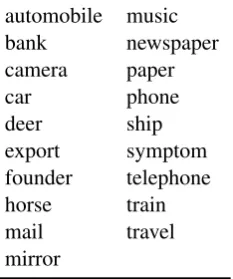
Table 6: Stable words from WSC Testset
automobile music
bank newspaper
camera paper
car phone
deer ship
export symptom
founder telephone
horse train
mail travel
mirror
E Closest Neighbors forShip
[image:13.595.125.242.317.457.2]Figure 8: Nearest neighbors forcomputer. Upper part SGNSAL, lower part SGNSTR.