A Gain Scheduled Method for Speed Control of Wind
Driven Doubly Fed Induction Generator
Wei Wang, Kang-Zhi Liu, Tadanao Zanma
Dept. of Electrical and Electronics Engineering, Chiba University, Chiba, Japan Email: [email protected]
Received 2013
Abstract
This paper proposes a gain scheduled control method for a doubly fed induction generator driven by a wind turbine. The purpose is to design a variable speed control system so as to extract the maximum power in the region below the rated wind speed. Gain scheduled control approach is applied in order to achieve high performance over a wide range of wind speed. A double loop configuration is adopted. In the inner loop, the rotor speed is used as the scheduling parameter, while a function of wind and rotor speed is used as the scheduling parameter in the outer loop. It is verified in simula-tions that a high tracking performance has been achieved.
Keywords: Doubly fed induction generator, Gain scheduled control method, speed control, current control
1.
Introduction
With rapid development of modern industries, fossil fu-els are being exhausted and environment is being de-stroyed seriously. For instance, burning of fossil fuels generates much waste carbon dioxide and causes global warming. As a solution to shortage of fossil fuels and environmental problems, much attention has been paid to the wind energy utilization because the wind energy is inexhaustible and has no emission of carbon dioxide and radioactive waste.
However, the wind energy is heavily influenced by weather and varies irregularly. Since the power captured by the wind turbine is proportional to the swept area and the cube of the wind speed, the utilization efficiency of wind power system becomes more and more important. In wind farms, doubly fed induction generator (DFIG) based doubly fed system and permanent magnet genera-tor (PMSG) based direct-drive system are generally in-stalled. Since DFIG is advantageous in lower cost and low power loss caused by power electronics device, it is widely used. As shown in Fig 1, DFIG system is differ-ent from convdiffer-entional wind power system in that its sta-tor is directly connected to the grid and the rosta-tor is con-nected to the grid through a back-to-back converter [1]. However, it is hard for the conventional linear control method to achieve high performance of DFIG systems in the case of large wind speed variation because of the high nonlinearity of wind power. So in recent years, non-
Fig 1: Block diagram of DFIG system.
linear control methods have been studied in order to im-prove the performance of DFIG. For example, [7] ap-plied the sliding-mode control to the direct active and reactive power regulation of DFIG. In [8] the exact li-nearization method is applied to the transient stability control of DFIG in face of fault. [9] proposed a combina-tion of PI control and state feedback nonlinear control so as to improve the dynamic behavior after clearing the fault.
In this paper, a gain scheduled method is proposed aiming at high performance in variable speed control which is indispensable in the maximum power point tracking. To this end, the nonlinear model of DFIG sys-tem will be transformed equivalently as an LPV model first. Then, a gain scheduled control method for the rota-tional speed control is proposed. Effectiveness of the method is verified by simulations. This method is
differ-grid-side converter R L rotor-side converter
DFIG gearbox
wind turbine
grid 3
rotor-side controller
ent from conventional variable speed control in that no approximation is made in model transformation.
2.
Operation modes of DFIG System
In general, a DFIG system has two operation modes which are described briefly below. Operation mode 1 is in the wind speed region between the cut-in wind speed and the rated wind speed. In this region, the pitch angle is fixed to 0, and the rotational speed of wind turbine is controlled in order to get better conversion efficiency [1]. Operation mode 2 is in the wind speed region between the rated wind speed and the cut-out wind speed. The control objective is to maintain the rated power by con-trolling the pitch angle as well as the rotational speed of wind turbine [2].
This paper deals with the rotational speed control of DFIG system in operation mode 1.
3.
Aerodynamic Characteristics
Tip speed ratio, which is used to evaluate the perfor-mance of the wind turbine, is defined as
R V ω λ = ⋅
(1)
where ωis the rotational speed of wind turbine, R is the
turbine radius, and V is the wind speed.
The power coefficient Cp(λ) represents the power
con-version efficiency of a wind turbine. In the case of oper-ation mode 1, the power and torque coefficients vary only with the tip speed ratio. The power coefficient is approximated as the following equation [3]:
21
116
( ) 0.5176 ( 5) 0.0068
1 1
0.035
i p
i
i
C λ e λ λ
λ
λ λ
−
= ⋅ − ⋅ +
= −
(2)
The relationship between the power coefficient Cp(λ)
and torque coefficient Cq(λ) is
( )
( ) p
q
C
C λ λ
λ
=
(3)
It can be seen from equation (2) that the maximum power coefficient is 0.48 and the optimal tip speed ratio is 8.10, at which the wind turbine can capture the wind energy with maximum efficiency. It also can be seen from equation (2) and equation (3) that the maximum torque coefficient is 0.0647 which is achieved at the tip speed ratio of 6.76. So the optimal rotational speed for a given wind speed is
8.10
opt V
R
ω = ⋅ (4)
According to equation (4), the optimal rotational speed may be computed by measurement of wind speed. The
maximum power point tracking may be implemented by setting the optimal rotational speed as the speed com-mand of the wind turbine. In addition, there also exist other methods which search the optimal rotational speed by means of search algorithms. In this paper, the first method is adopted in simulation because the focus here is on the rotational speed control.
4.
Model of Wind Turbine
The mechanical power of wind turbine is given by
2 3
1
( ) 2
m p
P = ρπR ⋅C λ ⋅V (5)
where ρ is the air density. The maximum power for a
given wind speed is
3
m opt p
P− =K ⋅V (6)
where Kp is determined by equation (5) with λopt=8.10
substituted into Cp(λ).
Moreover, the aerodynamic torque is given by
3 2
1
( ) 2
m q
T = ρπR C⋅ λ ⋅V (7)
5.
Dynamic Model of DFIG System
5.1.
DFIG Model
[image:2.595.313.532.492.581.2]The electric circuit configuration of DFIG is shown in
Fig 2, where uds and uqs denote the stator voltages, udr and
uqr denote the rotor voltages, ids and iqs denote the stator
currents, idr and iqr denote the rotor voltages, ψds andψqs
denote the stator fluxes and ψdr andψqr denote the rotor
fluxes in d-q frame. In modeling the stator and rotor of
DFIG, the motor convention is used.
Fig. 2: Circuit configuration of DFIG.
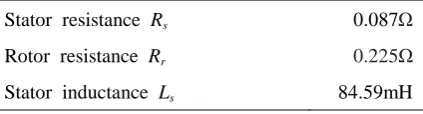
The values of physical parameters for DFIG studied here are illustrated in table 1.
Table 1. The values of physical parameters for DFIG.
Stator resistance Rs 0.087Ω
Rotor resistance Rr 0.225Ω
Stator inductance Ls 84.59mH
ubr
θre
ibr
stator A iar
ωre
icr
uar
ucr
ibs
ias
ics
uas
ubs
ucs stator A
[image:2.595.319.531.665.722.2]Rotor inductance Lr 85.71mH
Mutual inductance Lm 83Hm
Rated power 35kW
Rated voltages of stator and rotor 380V
The equivalent circuit of DFIG in the d-q reference
frame which rotates with synchronous speed ω1=2πf ( f :
power supply frequency) is used to set up the model eq-uations. The voltage equations of DFIG with constant
coefficients in the d-q reference frame are
1
1
ds s ds ds qs
qs s qs ds qs
dr r dr dr s qr
qr r qr s dr qr
u R i
u R i
u R i
u R i
ψ ω ψ ω ψ ψ ψ ω ψ ω ψ ψ = ⋅ + − ⋅
= ⋅ + ⋅ +
= ⋅ + − ⋅
= ⋅ + ⋅ +
(8)
The flux linkage equations with constant coefficients in
the d-q reference frame are
ds s ds m dr
qs s qs m qr
dr m ds r dr
qr m qs r qr
L i L i
L i L i
L i L i
L i L i
ψ ψ ψ ψ
= ⋅ + ⋅
= ⋅ + ⋅
= ⋅ + ⋅
= ⋅ + ⋅
(9)
The relationship between the slip frequency ωs and slip
s is defined as
1 1
s s np rm
ω
=ω
⋅ =ω
− ⋅ω
(10)where np and ωrmdenote the number of pole pairs and the
generator mechanical angular speed, respectively. The equations about the electromagnetic torque (driving torque) and the reactive power at the stator terminal are
( )
e p m qs dr ds qr
qs ds ds qs
T n L i i i i Q u i u i
= ⋅ ⋅ − ⋅
= ⋅ − ⋅
(11)
It is assumed that the stator of DFIG is connected to the constant-voltage constant frequency power supply
system. To realize decoupling control, d axis is aligned
with the grid voltage vector, which means
, 0
ds s qs
u =v u = (12)
after the commencement of electricity generation [4],
where vs is the magnitude of the grid voltage vector.
Since the voltage drop across the stator resistance is sufficiently low, it is neglected and the relationship between the stator voltage and flux is approximated as
1 , 0 1
s ds qs ds qs
v =ψ −ω ψ⋅ =ω ψ⋅ +ψ
(13)
It is assumed the stator flux has reached the steady state at the starting time of electricity generation, i.e.
1
( ) 0 , ( ) /
ds tci qs tci vs
ψ = ψ = − ω (14)
So after that, there holds
1
0 , /
ds qs vs
ψ = ψ = − ω (15)
By substituting equation (15) back into (9), the equa-tions of the stator and rotor currents become
1
,
m m s
ds dr qs qr
s s s
L L v
i i i i
L L ωL
= − ⋅ = − ⋅ −
(16)
Further, substitution of equation (16) into (11) yields the following electromagnetic torque and the reactive power [4]:
1
1
( )
p m s
e dr
s
m s
s qr
s s
n L v
T i
L
L v
Q v i
L L
ω
ω
= − ⋅
= ⋅ ⋅ +
(17)
It is easy to see that the electromagnetic torque is
pro-portional to idr and the reactive power at the stator
ter-minal is a linear function of iqr . Therefore, the
electro-magnetic torque Te is controlled by idr and the reactive
power Q is controlled by iqr. Hence, it is quite natural to
use a two-stage approach:
1. Control ω and Q by using idr and iqr respectively.
2. Design current feedback loops to track the current
commands computed in stage 1.
5.2.
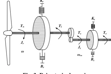
Drive-train Model
The schematic diagram of drive-train system is shown in
Fig 3, where Tl is the torsional torque at low-speed shaft
and Tg is the driving torque at high-speed shaft. Since the
stiffness coefficient Krand Kg are sufficiently low, it is
[image:3.595.331.510.441.560.2]neglected.
Fig. 3: Drive-train dynamics.
The values of physical parameters for drive-train sys-tem are illustrated in table 2.
Table 2. The values of physical parameters for drive-train system.
Inertia of wind turbine Jr 63 kg·m2
Inertia of DFIG Jg 4.97kg·m2
Damping coefficient of wind turbine Br 3.2Nms/rad
Damping coefficient of DFIG Bg 0.8Nms/rad
Br
Jg
ωrm
Kr
Tm Tl
Jr
Tg Te
Kg
Bg
Regarding the drive-train as a two-inertia system, the dynamic equations are obtained as
Fig. 4: Total control structure.
m l r r
g e g rm g rm
T T J B
T T J B
ω ω
ω ω
− = ⋅ + ⋅
+ = ⋅ + ⋅
(18)
Neglecting the power loss in gearbox, the following equ-ation is established according to the law of conservequ-ation of energy.
l g rm
T ⋅ =ω T ⋅ω (19)
The gearbox ratio is defined by
rm l
g
g
T n
T ω
ω
= = (20)
Substitution of equation (20) into (18) leads to the sim-plified model of drive train system [5].
2 2
,
m g e
r g g r g g
T n T J B
J J n J B B n B
ω ω
+ ⋅ = ⋅ + ⋅
= + ⋅ = + ⋅
(21)
6.
Controller Design for DFIG System
As shown in Fig.4, a double loop control configuration is adopted. In the inner loop, the current controller aims at high accuracy tracking of the reference rotor current, while in the outer loop, the rotational speed controller aims at capturing the wind energy with maximum effi-ciency and generates the reference rotor current. The controllers of these two loops are designed in this sec-tion.
6.1.
LPV Model for DFIG
Based on equation (8) and (9), an LPV model equivalent to the nonlinear model of DFIG is described as
(
)
:
ds ds
qs qs ds dr
p rm s r
dr dr qs qr
qr qr
rc
ds
dr qs
p dr qr
qr
i
i
i
i
u
u
d
A
B
B
i
i
u
u
dt
i
i
G
i
i
i
C
i
i
i
ω
=
⋅
+ ⋅
+ ⋅
=
⋅
(22)
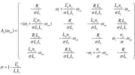
where Bs and Br are constant matrices, while Ap(ωrm) is
2
1
2 1
1
1
( )
( )
m p m p
s r m
rm rm
s s r s r s
m p s m p r m
rm rm
s r s s s r
p rm
m p p
s m r
rm rm
s r r r
m p s m p r
rm rm
r s r r
L n L n
R R L
L L L L L L
L n R L n R L
L L L L L L
A
L n n
R L R
L L L L
L n R L n R
L L L L
ω ω ω
σ σ σ σ
ω ω ω
σ σ σ σ
ω
ω ω ω
σ σ σ σ
ω ω ω
σ σ σ σ
σ
− + ⋅ ⋅
− + ⋅ − − ⋅
=
− ⋅ − − ⋅
⋅ − + ⋅ −
=
2
1 m
s r
L L L
−
and is affine in ωrm .
The size of power converter is not related to the total generator power but to the selected speed variation range.
Typically a range of ±40% around the synchronous
speed is used [1].
For f=50Hz, np=3 and ng=10, the speed of DFIG takes
value in ωrm=20π~140π/3 (rad/s) and the speed of wind
turbine takes value in ω=2π~14π/3 (rad/s), respectively.
R L
optimal speed calculation
reactive power measurement SVPWM bus voltage
controller
speed controller
reactive power controller rotor current
controller
Qref
Q
3 grid
ur
ir
gearbox rotor-side converter grid-side converter
DFIG
6.2.
Gain Scheduled Controller Design for Rotor
Current Control Loop
The generalized feedback system used for controller
de-sign is shown in Fig.5 in which Krc(s) is the gain
sche-duled controller.
The controlled output is selected as the tracking error of
rotor current (edr,eqr) and rotor voltage (udr,uqr), while
the stator voltage is treated as a disturbance.
The closed-loop system should achieve a high tracking performance in the low frequency band since the rotor reference current is majorly a low frequency signal, so
we select the weight functions Wsd(s) and Wsq(s) as low-
pass filters. Meanwhile the weight functions Wud(s) and
Wuq(s) are chosen as high-pass filters.
[image:5.595.332.508.166.286.2]
-+ +
Fig. 5: Generalized plant for rotor current control design.
Weighting functions are selected as follows through trial and error
100
( ) ( )
5.5 5 0.0001
( ) ( )
1000
sd sq
ud uq
W s W s
s s
W s W s
s
= =
+
= =
+
(23)
The state-space equation of generalized plant can be written as
1 2
1 11 12
2 21
( rm)
x A x B d B u
z C x D d D u
y C x D d
ω
= ⋅ + ⋅ + ⋅
= ⋅ + ⋅ + ⋅
= ⋅ + ⋅
(24)
where the disturbance vector d, the control input vector u,
the controlled output vector z and the measured output
vector y are as shown in Fig.5.
An output feedback control law which is affine in ωrm is
considered:
0 1 0 1
0 1 0 1
( ) ( )
( ) ( )
K K rm K K K rm K
K rm K K K rm K
x A A x B B y
u C C x D D y
ω ω
ω ω
= + ⋅ ⋅ + + ⋅ ⋅
= + ⋅ ⋅ + + ⋅ ⋅
(25)
where xK is the state vector of the controller.
An H∞ method is used in the design, i.e. we design an
output feedback control system whose L2 induced-gain
from d to z is minimized. The design specification is
re-duced to LMIs at the maximum and minimum values of
ωrm in its operating range, and solved numerically [6].
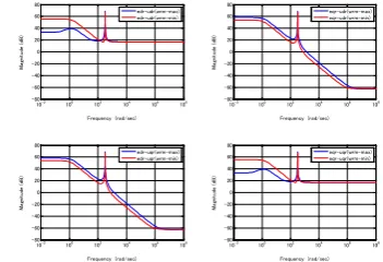
The bode plots of rotor current controller for the
maxi-mum (blue lines) and minimaxi-mum (red lines) values of ωrm
are shown in Fig.6. It can be seen from this figure that
the magnitudes of frequency response vary with ωrm
sub-stantially.
10-2 100 102 104 106 108
-80 -60 -40 -20 0 20 40 60 80
M
ag
ni
tud
e
(d
B
)
Frequency (rad/sec)
10-2
100
102
104
106
108
-80 -60 -40 -20 0 20 40 60 80
M
ag
ni
tud
e
(d
B
)
Frequency (rad/sec)
10-2 100 102 104 106 108
-80 -60 -40 -20 0 20 40 60 80
M
ag
ni
tud
e
(d
B
)
Frequency (rad/sec)
10-2
100
102
104
106
108
-80 -60 -40 -20 0 20 40 60 80
M
ag
ni
tud
e
(d
B
)
Frequency (rad/sec) edr-udr(wrm-max)
edr-udr(wrm-min) eqr-udr(wrm-max)eqr-udr(wrm-min)
edr-uqr(wrm-max)
edr-uqr(wrm-min) eqr-uqr(wrm-max)eqr-uqr(wrm-min)
Fig. 6: Bode gain plots of rotor current controller.
6.3.
LPV Model for Drive-train System
Substitution of equation (7) into (21) leads to an LPV model of drive train system in the operating range from the cut-in wind speed to the rated wind speed.
: dr
s
B
M p K i
P J
y
ω ω
ω
= − + ⋅ ⋅ + ⋅
=
(
26)
where
3
1
, 2
g p m s
s
n n L v R
M K
J J L
ρπ
ω
= = − ⋅
The scheduling parameter p is defined as
2
( )
q
V p C λ
ω
= ⋅
(27)
It is assumed that the wind speed is measured. So p can
be computed on-line and takes value in p=0~1.03.
6.4.
Gain Scheduled controller Design for
Rotational Speed Control Loop
The generalized feedback system shown in Fig.7 is used for rotational speed controller design.
[image:5.595.67.273.270.384.2]-+
Fig. 7: Generalized plant for rotational speed controller design.
Wud
Wuq
G
rcKrc
d z
Wsd
Wsq
Ws
Wu
P K
[image:5.595.334.508.590.685.2]Similarly to the rotor current control design, the con-trolled output is selected as the tracking error of
rotation-al speed ωref-ωand the d component of rotor current i
dr.
The weighting functions are selected as follows through trial and error
0.1 1
( )
2.85 0.001
12.4 31
( )
3 800
s
u
s W s
s s W s
s
+
=
+
+
=
+
(28)
The gain scheduled controller has the form below
0 1 0 1
0 1 0 1
( ) ( )
( ) ( )
K K K K K K
K K K K K
x A p A x B p B y
u C p C x D p D y
= + ⋅ ⋅ + + ⋅ ⋅
= + ⋅ ⋅ + + ⋅ ⋅
(29)
The numerical design is similar to that of the rotor cur-rent loop [6].
7.
Simulation Results
In simulations, an integrator controller 0.5
Q
K s
= (30)
is used as the reactive power controller. The reactive power command is set as
100 var 0 350
250 var 350 700
550 var 700 1000
ref
s t s
Q s t s
s t s
− ≤ <
= − ≤ <
− ≤ ≤
(31)
The command of rotational speed is computed by equa-tion (4) in which the wind speed is given in Fig.8.
Simulations results are shown in Fig. 8~Fig. 13 in the case where the wind speed input is a rapidly changing random signal.
0 100 200 300 400 500 600 700 800 900 1000
6.500 7.000 7.500 8.000 8.500 9.000 9.500
W
ind
s
p
eed
(m/
s
)
0 100 200 300 400 500 600 700 800 900 1000
0.472 0.474 0.476 0.478 0.480 0.482
P
o
w
er
co
ef
fi
ci
ent
time (s)
Wind speed
[image:6.595.316.518.94.234.2]Maximum power coefficient Real value
Fig. 8: Wind speed (top) and power coefficient (bottom).
As shown in Fig.8, the power coefficient is almost not influenced by the irregular variation of the wind speed and has been maintained close to its maximum value.
0 100 200 300 400 500 600 700 800 900 1000
8.50 9.50 10.5 11.5 12.5 13.5
R
o
ta
ti
o
na
l s
p
eed
o
f w
ind
t
ur
b
ine (
ra
d
/s
)
0 100 200 300 400 500 600 700 800 900 1000
-0.80 -0.50 -0.20 0.10 0.40
time (s)
E
rror of
rot
a
ti
on
a
l s
p
e
e
d
(
ra
d
/
s
)
Error of rotational speed
Reference value Real value
Fig. 9: Rotational speed of wind turbine (top) and tracking error of rotational speed (bottom).
0 100 200 300 400 500 600 700 800 900 1000
10.0 15.0 20.0 25.0 30.0
W
ind
t
ur
b
ine p
o
w
er
(KW
)
0 100 200 300 400 500 600 700 800 900 1000
0.00 0.60 0.12 0.18 0.24 0.30
time (s)
E
rror of
w
ind
t
ur
b
ine p
o
w
er
(
K
W
)
Reference value Real value
[image:6.595.314.518.174.427.2]Error of wind turbine power
Fig. 10: Wind turbine power (top) and tracking error of wind turbine power (bottom).
It can be confirmed from Fig.9 and Fig.10 that a high tracking performance of rotational speed and the max-imization of wind energy capture have been achieved.
0 100 200 300 400 500 600 700 800 900 1000
-0.6 -0.4 -0.2 0.0 0.2 0.4
R
ea
ct
iv
e p
o
w
er
(K
var
)
0 100 200 300 400 500 600 700 800 900 1000
-0.6 -0.4 -0.2 0.0 0.2
time (s)
E
rror of
re
ac
ti
ve
p
o
w
e
r (
K
var
[image:6.595.62.266.485.643.2]) Error of reactive power Reference value Real value
[image:6.595.315.516.518.692.2]The response of the reactive power is shown in Fig.11, in which it can be seen that the reactive power has achieved a high accuracy tracking of the command.
0 100 200 300 400 500 600 700 800 900 1000
0.00 5.00 10.0 15.0 20.0
d a
x
is
rot
or c
u
rre
n
t (
A
)
0 100 200 300 400 500 600 700 800 900 1000
-26.5 -26.0 -25.5 -25.0 -24.5
time (s)
q a
x
is
rot
or c
u
rre
n
t (
A
)
d axis rotor current
q axis rotor current
Fig.12: d axis rotor current (top) and q axis rotor current (bottom).
As shown in Fig.12, idr varies with the wind speed while
iqr varies with the command of reactive power. The high
frequency component in the rotor currents is suppressed efficiently.
0 100 200 300 400 500 600 700 800 900 1000
-200.0 -130.0 -60.00 10.00 80.00 150.0
d a
x
is
rot
or v
ol
ta
g
e
(
V
)
0 100 200 300 400 500 600 700 800 900 1000
-12.00 -9.000 -6.000 -3.000 0.000
time (s)
q a
x
is
rot
or v
ol
ta
g
e
(
V
)
d axis rotor voltage
q axis rotor voltage
Fig.13: d axis rotor voltage (top) and q axis rotor voltage (bottom).
Finally, Fig.13 shows that the high frequency
compo-nent in the rotor voltages is suppressed efficiently and the variation is in a reasonable range.
8.
Conclusion
This paper has proposed a gain scheduled control method for a doubly fed induction generator driven by a wind turbine. This method is based on equivalent LPV
model-ing of the nonlinear DFIG system and H∞ optimization. It
is confirmed by simulations that a quite high precision tracking control of rotor speed as well as reactive power is achieved by the proposed method.
As a future work, we plan to deal with the controller design for DFIG systems operating in mode 2 in order to maintain the rated power.
REFERENCES
[1]
“Optimal control of wind energy systems,” Springer, 2008.
[2] F.D. Bianchi, H.De. Battista and R. J.Mantz, “Wind tur-bine control systems: principles, modeling and gain scheduling design,” Springer, 2006.
[3] A. Monroy, L. Alvarez-Icaza,
45th IEEE
confe-rence on
[4] N.P. Quang, A. Dittrich and A. Thieme, “Doubly-fed induction machine as generator: control algorithms with decoupling of torque and power factor,” Electrical Engi-neering, 1997, 325-335.
[5] B. Boukhezzar and H. Siguerdidjane, “Nonlinear control of variable speed wind turbines without wind speed mea-surment,” Proceedings of the 44th IEEE conference on decision and control, 2005, 3456-3461.
[6] P. Gahinet, A. Nemirovski, A. Laub and M. Chilali, “The LMI Control Toolbox,” The Mathworks, Inc, 1995 [7] J. Hu et al., “Direct active and reactive power regulation
of DFIG using sliding-mode control approach,” IEEE Trans. on Energy Conversion, vol. 25, no. 4, pp.1028 -1038 (2010. 12)
[8] F. Wu et al., “Decentralized nonlinear control of wind turbine with doubly fed induction generator,” IEEE Trans. on Power Systems, vol. 23. no. 2, pp613-621 (2008. 5) [9] M. Rahimi and M. Parniani, “Transient performance