Munich Personal RePEc Archive
Sharp and Smooth Breaks in Unit Root
Testing of Renewable Energy
Consumption: The Way Forward
Shahbaz, Muhammad and Omay, Tolga and Roubaud, David
Montpellier Business School, Montpellier, France, Atilim University,
Department of Economics, Ankara, Turkey, Montpellier Business
School, Montpellier, France
5 February 2019
Online at
https://mpra.ub.uni-muenchen.de/92176/
Sharp and Smooth Breaks in Unit Root Testing of Renewable Energy Consumption: The Way Forward
Muhammad Shahbaz
Montpellier Business School, Montpellier, France Email: [email protected]
Tolga Omay
Atilim University, Department of Economics, Ankara, Turkey Montpellier Business School, Montpellier, France
Email: [email protected]
David Roubaud
Montpellier Business School, Montpellier, France Email: [email protected]
Abstract: This study proposes a flexible unit root test that detects sharp and smooth breaks
simultaneously. Most unit root tests are not general enough to capture different dynamics, such as smooth structural breaks, sharp structural breaks, state-dependent nonlinearity or a mixture of them. Therefore, considering all these data structures in one unit root process is important, and the results produced with this type of test structure do not face misspecification problems. We test 9 countries’ historical renewable energy consumption covering the period of 1800-2008 with traditionally used structural break unit root tests and a newly proposed test. The newly proposed test performs better than the traditional ones. The reason is that renewable energy consumption has sharp and smooth breaks in its data generating process which are not captured simultaneously by any other traditional unit root test. The empirical results indicate that renewable energy consumption contains stationary process in the presence of sharp and smooth structural breaks.
Keywords: Unit Root Testing, Sharp and Smooth Break, Renewable Energy Consumption
1. Introduction
Energy demand has increased rapidly as a result of globalization, urbanization and
industrialization in emerging and developing economies (Ozcan and Ozturk 2016, Shahbaz et
al. 2017). This has led researchers, academicians and practitioners to investigate the unit root
properties of energy consumption in a new research area pioneered by Narayan and Smyth
2007) in energy economies. Testing the unit root properties of energy consumption is
important, as energy consumption is closely linked with economic growth and environment
(Ozcan and Ozturk, 2016). A plethora of empirical studies have investigated whether energy
consumption contains a unit root process, but they provide conflicting empirical findings
(Shahbaz et al. 2014, Ozturk and Aslan 2015, Ozcan and Ozturk 2016). Understanding the
unit root properties of energy consumption is crucial for researchers, practitioners and policy
makers to maintain the energy supply by designing comprehensive energy policies for
sustainable economic development over a long time span (Ozturk and Aslan, 2015).
The testing of the time series stationary properties of energy consumption has many
policy implications for the design of energy policy: (i) if energy consumption follows a
stationary process, then shocks to the global energy market will have temporary or transitory
effects on energy consumption. In such circumstances, a shock to energy consumption results
in a temporary deviation from the long-run path, and energy consumption returns to its trend
path after a certain time (Hsu et al. 2008, Kula et al. 2012). This suggests that governments
should avoid the unnecessary adoption of energy targets, as energy consumption deviates
from the long-run path temporarily. In such situations, the implementation of energy
conservation and energy management policies for reducing energy intensity or consumption is
meaningless in the long run (Kum 2012, Ozturk and Aslan 2015, Shahbaz et al. 2016).
Apergis and Payne (2010) explain that energy conservation and management policies, i.e.,
transportation, will have transitory effects, as oil consumption contains a stationary process,
and oil consumption will revert to the mean. If energy consumption contains a unit root or
random walk process, then shocks to the global energy market will have permanent and
long-run effects on energy demand or energy consumption. This is termed the hysteresis hypothesis
in energy consumption or energy demand (Narayan and Smyth 2007, Barros et al. 2013,
Shahbaz et al. 2016). In such circumstances, shocks to energy consumption affect economic
activity permanently and, energy exploring and energy management policies designed for
energy supply will be effective.
Based on the close linkage between energy demand and real economy, the presence of
structural breaks, i.e., the outcomes of government policies in energy markets, may cause
fluctuation in macroeconomic variables. In such circumstances, permanent shocks to energy
consumption may cause a unit root process in other macroeconomic variables, such as
domestic production, employment, inflation, trade and the exchange rate via the transmission
mechanism (Narayan and Smyth 2007, Mishra et al. 2009, Shahbaz et al. 2014). Hendry and
Juselius (2000) argue that “variables related to the level of any variables with a stochastic
trend will inherit that nonstationary and transmit to it other variables in turn”. This
invalidates some economic theories. For instance, real business cycle theory implies that the
real output contains a stationary process that indicates the transitory shocks to real output
(Hamilton 1996, Sardosky, 1999, Hasanov and Telatar 2011)1. Similarly, permanent shocks to the unit root process in oil consumption transmit to economic activity, which invalidates the
empirical support of oil price shocks and real business cycle theories (Ozcan and Ozturk
2015). In international trade, the law-of-one-price theory accepts exchange rates as stationary,
and conventional sticky price models developed by Dornbusch (1976) and Taylor (1979)
assume that the price level contains a stationary process. The presence of a random walk
1 Narayan et al. (2010) report that if energy consumption contains a unit root process via a transmission
process in energy consumption may invalidate these economic theories as we use
transmission mechanisms to explain direct and indirect linkages between energy and
macroeconomic variables.
Testing the unit root properties of energy consumption is crucial for forecasting future
energy demand. The forecasting of energy consumption is considered a basic tool for
formulating policy on energy management and planning (Chen and Lee 2007, Mishra et al.
2009, Aslan 2011). The mean contains a reverting process to the trend path if energy
consumption contains a stationary process. In such a situation, the past trend of energy
consumption might be used to forecast energy demand (Chen and Lee 2007, Apergis et al.
2010, Shahbaz et al. 2014). The past behaviour of energy consumption is useless for forecasts
of future energy demand if energy consumption has a unit root problem, i.e., energy
consumption does not return to the trend path. This shows that other macroeconomic variables
explaining energy consumption are important for generating forecasts of future energy
consumption (Shahbaz et al. 2014, Ozcan and Ozturk 2015).
Last but not least, testing the unit root properties of energy consumption will be
helpful in applying time series approaches, such as cointegration and causality tests, for
empirical analysis (Shahbaz et al. 2013). Furthermore, the stationary properties of energy
consumption play an important role in modelling the association between energy consumption
and macroeconomic variables, such as output growth (Hasanov and Telatar 2011, Liu 2013,
Smyth 2013, Yilanci and Tunali 2014, Wang et al. 2016). If all variables contain a stationary
process, then a vector autoregressive (VAR) model is suitable to empirically examine the
long-run relationships between the variables2. If the variables contain a unit root process, we have three options: (i) The VAR model in differences is a suitable way to model the
relationships between the variables, as there is an absence of cointegration between the series
(Hendry and Juselius 2000, Hasanov and Telatar 2011, Liu 2013). (ii) The vector error
correction (VEC) is applicable as variables are integrated at I(I). For example, Granger (1969)
argues that if the variables are integrated at I(1), then the VECM Granger causality version of
unrestricted VAR is suitable to examine the long-run and short-run causal associations
between the variables. (iii) If the variables contain a unique order of integration, the Johansen
and Juselius (1990) cointegration approach is suitable to examine the cointegration
relationships between the variables. The bounds testing approach to cointegration developed
by Pesaran et al. (2001) is also suitable if the variables have a mixed order of integration, i.e.,
I(1)/I(0)3. Additionally, modelling the association between energy consumption and economic growth shows the vital role of energy consumption in economic growth (Oh and Lee, 2004).
For instance, causality runs from energy consumption to economic growth, which indicates
that energy consumption leads to economic growth or that energy consumption is a driver of
economic growth. In such a situation, the implementation of energy conservation policies
would impede economic growth by de-fuelling economic activity.
Following conflicting empirical results as reported in Table-1, this paper consequently
contribute to the existing energy economics by two major folds: (i), This paper uses long
historical data for the period of 1800-2008 in order to examine the unit root properties of
renewable energy consumption for Canada, France, Germany, Italy, the Netherlands,
Portugal, Spain, Sweden, and the UK4. (ii), This study also enriches by means of a unit root test which accounts potential sharp shifts and smooth breaks stemming in renewable energy
consumption. It is documented that the persistence parameter of a process may be
overestimated if structural breaks are omitted or disregarded from unit root analysis,
subsequently decreasing the explanatory power to reject a unit root when the stationarity
alternative is true (Perron, 1989). Therefore, we model breaks in our unit root testing process,
with the structure changes being both smooth and sharp, given that we use very long historical
yearly data, and hence, both types of structural breaks are possibly to co-exist. Our procedure
also allows us to model sharp breaks endogenously, unlike standard dummy variable unit root
tests which only permit exogenous determination. Therefore, our methodology allows more
flexible testing structure when there is no sharp break available in the data, thereby the
methodology does not account for sharp break. While at the same time, we have the same
flexibility in the smooth structural break methodology. The Fourier function parameters are
not significant when there is no smooth break is available, hence, the testing procedure does
not account for smooth break, as well. Thus these features make our testing procedure more
general and flexible. Moreover, our methodology is also efficient (powerful) in which the data
generating process (DGP) is containing sharp structural break in isolation or any other
features of DGP such as state dependent nonlinearity, smooth shifts and/or linear DGP. These
properties of our unit root testing procedure give opportunity to a researcher to safely analyse
wide variety of datas’ stationarity features in more flexible and general setting.
Finally, increasing economic activity boosts energy demand and the environmental
constraints such as increasing CO2 emissions restricts energy consumption. Therefore, in a long span data, this dynamic may create a sharp break which cannot be captured by smooth
shifts. When we looked at the 9 developed countries data from 1800s until 1940s there occur a
smooth, nearly horizontal trend which can be captured by simple linear trend, however, after
the Second World War renewable energy consumption is triggered and the trend become
nearly vertical until 1980. This sharp shift cannot be captured by simple linear trend or any
other function which can captured smooth structural break, hence, this period dynamics can
be classified as sharp structural break or shift. The recovery period of the world economy
after Second World War is slowdown in 1980s which we can be classified as the liberalization
and the slope of energy consumption becomes more horizontal relatively to recovery period,
but steeper than before the Second World War era. In the meanwhile, we also see some
smooth breaks in all 9 countries renewable energy consumption. For example in between
1940-1945 nearly all countries energy demand falls for a short period due to Second World
War and similar short period decrease is also seen in 1973 oil crises. These, short period
swings are also occurred due to business cycles as we have mentioned before and has seen in
renewable energy consumption data of 9 developed countries. Finally, after 1990s depending
on environmental pollutions and deterioration most of developed countries shift their
industrial production to less developed areas which is also cause a decline in energy demand
thereby creates small breaks in renewable energy consumption data of sampled countries.
These stylized facts which we have documented show that renewable energy
consumption follows some deterministic pattern. Therefore, if these deterministic patterns can
be captured with unit root testing procedures, then we prevent our self to accepting wrong
non-stationarity hypothesis of renewable energy consumption. The numerous dynamics which
are explained in the previous paragraph cannot be captured by a linear or state dependent or
structural break unit root tests in isolation. Therefore, our hybrid, flexible and more general
approach is the only right procedure to capture these varieties of dynamics to lead us for
making correct decision on stationary properties of renewable energy consumption for
sampled countries, otherwise, we may accept the unit root hypothesis and give rise to policy
makers to take wrong policy actions.
The rest of the paper structured as follows. Section 2 presents the literature review,
section 3 introduces the new unit root test, section 4 outlines the empirical study, and section
2. Literature review
Narayan and Smyth (2007) started the debate on testing the unit root properties of
energy consumption. Subsequently, researchers have focused on investigating the stationary
properties of energy variables, such as energy consumption. Table-1 contains a summary of
studies in the literature that have investigated unit root testing of energy consumption. Most of
the studies have produced mixed results regarding stationary and unit root processes in energy
consumption. These conflicting results are the outcome of the samples, countries and unit root
tests chosen. These unit root tests are not free from criticism. For example, Narayan and
Smyth (2007) applied the ADF unit root test to examine the unit root properties of energy
consumption. This test provides ambiguous empirical findings as it ignores the role of
structural breaks in the series, which may be the cause of the unit root problem. This test has
low explanatory power and thus is not suitable for small data sets (Ng and Perron, 2001).
These disadvantages of the ADF unit root test call into question the empirical findings of
Narayan and Smyth (2007) and Hasanov and Telatar (2011). The Langrage Multiplier (LM)
was developed by Schmidt and Phillips (1992) and has been applied by numerous researchers,
such as Aslan and Kum (2011), Ozturk and Aslan (2015), Kum (2012), Bolat et al. (2013),
Ozcan (2013), Lean and Smyth (2014), Shahbaz et al. (2015) and Wang et al. (2016), to
examine the unit root properties of energy consumption; however, the results are ambiguous.
This test is suitable for restricted and linear models, imposing a significant demand on
parameter estimations. The LM unit root test requires accurate estimates of parameter
covariance, which is a main disadvantage of it. Therefore, the empirical findings on the LM
unit root test are doubtful. The minimum LM unit root test by Lee and Strazicich (2003),
which accommodates two unknown structural breaks in the time series, has been employed by
Apergis and Payne (2010), Narayan et al. (2010), Aslan (2011), Kula et al. (2012) and Gozgor
(2003) test is superior to the ADF and LM unit root test, but its issue is that the economic
implications of two structural breaks in a time series are difficult to identify while testing the
unit root process. Similarly, Chen and Lee (2007), Hsu et al. (2008), Mishra et al. (2009), Liu
(2013) and Magazzino (2016) applied the C-S (Carrion i Silvestre et al. 1999), SURADF
(Breuer et al. 2001), KSS (Kapetanios et al. 2003) and IPS (Im et al. 2003) unit root tests to
investigate whether shocks to energy consumption are temporary or permanent. These unit
root tests are also not free from criticism and provide vague empirical results.
Table-1: Summary of Studies on Unit Root Analysis
No. Author(s) Time Period Unit Root Test Conclusion
1 Narayan and Smyth (2007) 1979-2000 ADF Unit root process.69% count.
2 Chen and Lee (2007) 1971-2002 C-S Stationary
3 Hsu et al. (2008) 1971-2003 SURADF Mixed Evidence
4 Mishra et al. (2009) 1980-2005 C-S Mixed Evidence
5 Apergis and Payne (2010) 1960-2007 LS Mixed Evidence
6 Narayan et al. (2010) 1973-2007 LS Stationary
7 Aslan (2011) 1960-2008 LS Mixed Evidence
8 Aslan and Kum (2011) 1970-2006 LM Unit Root Process
9 Hasanov and Telatar (2011) 1980-2006 ADF. KSS. ST-TAR Stationary
10 Kula et al. (2012) 1960-2005 LS Mixed Evidence
11 Kum (2012) 1971-2007 LM Stationary
12 Bolat et al. (2013) 1971-2010 LM Stationary
13 Liu (2013) 1963-2009 KSS Stationary
14 Ozcan (2013) 1980-2009 LM Stationary
15 Ozturk and Aslan (2015) 1970-2006 LM Mixed Evidence
16 Yilanci and Tunali (2014) 1960-2011 FLM Mixed Evidence
17 Lean and Smyth (2014) 1975-2008 LM Mixed Evidence
18 Shahbaz et al. (2015) 1965-2010 LM Mixed Evidence
19 Wang et al. (2016) 1965-2011 LM Mixed Evidence
20 Gozgor (2016) 1971-2014 LS Mixed Evidence
21 Magazzino (2017a) 1960-2013 IPS Unit Root Process 22 Magazzino (2017b) 1971-2013 CADF Mixed Evidence 23 Edmir and Gozgor (2017) 1971-2016 N-P Unit Root Process
Note: ADF, SURADF, C-S, W, LS, LM, FLM, KSS, ST-TAR, and IPS refer to Augmented Dickey-Fuller, Seemingly Unrelated Regressions ADF, Carrion i Sivestre, Westerlund, Lee and Strazicich, Langrage Multiplier, Fourier LM, Kapetanios, Shin and Shell, Stationary Smooth Transition Threshold Autoregressive, and Im, Pesaran and Shin, Cross-sectional ADF, Narayan and Popp (2010) respectively.
The most important thing to do while performing a unit root test is to employ a true
data-generating process in the unit root-testing process. The studies shown in Table-1 aimed to
employ true unit root tests for a true sample period with true country groups, which means
unit root tests are not general enough to capture different dynamics, such as smooth structural
breaks, sharp structural breaks, state-dependent nonlinearity or a mixture of them. The
available tests in the literature target these data-generating processes one at a time. For
example, the KSS test considers only state dependent nonlinearity. The LS test considers only
multiple smooth structural breaks. The ST-TAR considers one smooth break and the TAR
type of state-dependent mixed nonlinearity; although the ST-TAR unit root test is the most
general one, it still includes one smooth structural break and a very restricted type of
state-dependent nonlinearity. Therefore, considering all these data structures in one unit root
process is important, and the results produced by this type of test structure do not face
misspecification problems. As indicated by Table-1, energy consumption has different
dynamics in different countries and different samples. Therefore, it is better to understand the
historical perspective of renewable energy consumption.
We know that renewable energy consumption has faced various types of structural breaks
in the course of its history, starting with the Industrial Revolution, due to technological
improvements or the dynamics of the business cycle, which directly affect the use of energy.
It is important to understand historical data in order to understand the stochastic properties of
energy use. Many studies use a short data timespan to analyse the stochastic properties of
energy use, but this approach gives a very limited picture of the real data-generating process
of energy consumption. Therefore, in this study, we use a very long historical data period,
starting from 1820, which can be classified as the start of the Industrial Revolution. This
novel data set can foster our understanding of the stochastic behaviour of energy use.
However, to understand this long-span data, we must have very flexible method that can
detect smooth and sharp breaks in the data-generation process. Plenty of studies have
proposed the unit root test for sharp and smooth breaks. Furuoko (2016) uses a dummy
sharp breaks is problematic in two ways. First, the exogenous determination of structural
breaks requires another method or visual inspection, which limits the power of the test.
Second, using a dummy variable creates discontinuity in de-trending data or nonlinear trends,
which may be other important problem. Moreover, he does not use trend breaks in his
modelling, which is also another limitation in his modelling of sharp breaks. In our modelling,
we eliminate all of these problems. The other strand of literature on Fourier transforms claims
to detect sharp and smooth breaks in the data by increasing the number of Fourier transforms,
N (Enders and Holt, 2012). This methodology has its own problems, as documented by the
same authors (Becker et al. 2006, Enders and Lee, 2012a, b). They note that the increasing
number of Fourier transforms (cumulative) captures sharp breaks, but this process also creates
a problem: the newly added Fourier function over-fits the data and induces an over-filtration
problem, especially in the stochastic part of the series. Thus, we propose a more flexible
method that solves all the mentioned problems in two steps.
3. Methodological Framework
3.1 The model and testing framework
Let yt be a changing trend function with a smooth transition on the time domain
1, 2,..., t= T.
Model A: yt = +α α1 2Ft
( )
γ τ ε, + t (1)Model B: yt = +α β α1 1t+ 2Ft
( )
γ τ ε, + t (2)whereεt is a zero mean I
( )
0 process, and Ft( )
γ τ, is the following the LST function, basedon a sample of size T:
( )
γ τ, =1 / 1 exp+ −γ(
−τ)
t
F t T ,
γ
>0 (4)In this modelling strategy, the structural change is modelled as a smooth transition
between different regimes5. In these specifications, no change and one instantaneous and, sharp structural change are limiting cases6. Following Leybourne et al. (1998), the test statistics proposed here are calculated with a two-step procedure:
Step 1. Using constrained nonlinear optimization algorithm via Genetic7, we estimate only the
deterministic component of the preferred model and compute its residuals.
( )
1 2
ˆ ˆ ˆ ˆ ˆ
Model A :εt = − −yt α α Ft γ τ, (6)
( )
1 ˆ1 2
ˆ ˆ ˆ ˆ ˆ
Model B :εt = − +yt α βt−α Ft γ τ, (7)
( )
( )
1 ˆ1 2 ˆ2
ˆ ˆ ˆ ˆ ˆ ˆ ˆ
Model C :εt = − −yt α βt−α Ft γ τ, −β Ft γ τ, t (8)
Step 2. Compute the Enders and Lee (2012) (Henceforth, EL test) statistic, which is the t ratio
associated withφˆ in the ordinary least squares regression:
1 1
ˆt d t( ) ˆt t
ε = +φ ε − +υ (9)
5For details, see Omay and Emirmahmutoglu (2017).
6 For further discussion and possible extensions, see Leybourne et al. (1998).
7We use the genetic algorithm in our estimation process of the smooth transition trend since it is shown to be the
whereυt is a stationary disturbance with variance
σ
2, and d t( )is a deterministic function oft. We note that the initial value is assumed to be a fixed value, and εt is weakly dependent. If
the functional form of d t( ) is known, it is possible to estimate equation-9 directly and to test
the null hypothesis of a unit root (i.e.φ1=1). When the form of d t( )is unknown, any test for
1 1
φ = is problematic if d t( ) is mis-specified. This unit root test is based on the fact that it is
often possible to approximate d t( )using the Fourier expansion:
0
1 1
2 2
( ) sin cos
,
/ 2n n
k k
k k
kt kt
d t n T
T T
π π
α α β
= =
= + + ≤
∑
∑
(10)wheren represents the number of cumulative frequencies contained in the approximation, k
represents a particular frequency, and Tis the number of observations. In the absence of a
nonlinear trend, all values of αk =βk =0 so that the LNV (1998) specification emerges as a
special case. There are several reasons why it is inadvisable to use a large value for n. As we
demonstrate below, the presence of many frequency components uses degrees of freedom and
can lead to an over-fitting problem. As evidenced by Gallant (1981), Davies (1987), Gallant
and Souza (1991) and Bierens (1997), a Fourier approximation using a small number of
frequency components can often capture the essential characteristics of an unknown
functional form smooth break. Moreover,n should be small since8 it is important to allow the
8
evolution of the nonlinear trend to be gradual. There is little point in claiming that a series
reverts to an arbitrarily evolving mean. The testing equation is finally as follows:
0 1 1
1 1 1
2 2
ˆ sin π cos π ˆ ˆ
ε α α β φ ε − ϕ ε− υ
= = =
∆ = + + + + ∆ +
∑
n∑
n∑
pt k k t k t i t
k k i
kt kt
T T (11)
where the common practice is to augment the dependent variables’ lag value in testing the
equation to account for any stationary dynamics in ˆεt. Therefore, we denote value of this EL
test statistic as sταif Model A is used to construct ˆεt, sτα β( )if Model B is used, andsτα β, if
model C is used.
One key issue for our test is whether a small number of frequency components can
replicate the types of breaks typically observed in economic data. To keep the problem
tractable, we begin by considering a Fourier approximation using a single frequency
component so that k represents the single frequency selected for the approximation, and αk
and βk measure the amplitude and displacement of the sinusoidal component of the
deterministic term. Thus, even with a single frequency k=1, we can allow for multiple
smooth breaks. The established hypotheses of unit root testing based on models A, B and C
with the Fourier transforms are as follows:
(
)
0: Linear Nonstationary
H Unit Root
(12)
1
Nonlinear and Stationary around
simultenously changing sharp and smooth trend
:
H Nonlinear Stationary
The critical values for the newly proposed test with trends in the Fourier function are
functions. Therefore, including trends in the second step is useless. However, we include the
trend in the Fourier function for Model Abecause there is no trend variable in Model A of the
smooth transition trend. This model is probably a competitor of Model B. We tabulate the
value of Model A* in Appendix A.2 with Fourier transforms, which also includes trend
functions. Additionally, we do not generate the critical values for the cumulative Fourier
function because the LNV function captures the sharp breaks without including any other
term. Table-2 consists the critical values for Model A (sτα), B (sτα β( )) and C (sτα β, ).
Table-2: Critical Values for FLST Models only Intercept Included in Fourier Function9
α
τ
s sτα β( ) sτα β,
T 1% 5% 10% 1% 5% 10% 1% 5% 10%
k=1
25 -5.658 -4.777 -4.323 -6.085 -5.184 -4.747 -6.794 -5.596 -5.150 50 -5.288 -4.484 -4.139 -5.515 -4.804 -4.450 -5.826 -5.127 -4.788 100 -4.926 -4.394 -4.081 -5.189 -4.625 -4.354 -5.549 -4.965 -4.670 200 -4.941 -4.323 -4.037 -5.138 -4.585 -4.317 -5.405 -4.859 -4.579 500 -4.807 -4.281 -4.007 -5.129 -4.513 -4.273 -5.345 -4.810 -4.518 k=2
25 -5.955 -4.985 -4.554 -6.530 -5.506 -5.061 -6.885 -5.871 -5.412 50 -5.453 -4.730 -4.389 -5.705 -5.079 -4.751 -6.040 -5.373 -5.016 100 -5.206 -4.614 -4.312 -5.459 -4.892 -4.567 -5.726 -5.141 -4.851 200 -5.065 -4.528 -4.233 -5.369 -4.788 -4.522 -5.587 -5.031 -4.750 500 -4.997 -4.480 -4.192 -5.227 -4.711 -4.436 -5.563 -5.020 -4.704 k=3
25 -6.048 -4.990 -4.527 -6.677 -5.631 -5.149 -7.076 -6.081 -5.599 50 -5.450 -4.743 -4.368 -5.870 -5.187 -4.828 -6.240 -5.497 -5.175 100 -5.206 -4.614 -4.262 -5.583 -4.976 -4.661 -5.889 -5.276 -4.974 200 -5.104 -4.476 -4.185 -5.396 -4.866 -4.582 -5.697 -5.124 -4.827 500 -5.029 -4.484 -4.172 -5.330 -4.821 -4.540 -5.607 -5.073 -4.792 k=4
25 -5.884 -4.870 -4.365 -6.637 -5.507 -5.016 -7.072 -6.022 -5.526 50 -5.398 -4.614 -4.209 -5.919 -5.125 -4.737 -6.234 -5.515 -5.131 100 -5.183 -4.504 -4.156 -5.587 -4.917 -4.590 -5.860 -5.255 -4.939 200 -5.042 -4.435 -4.099 -5.401 -4.847 -4.533 -5.670 -5.110 -4.816 500 -4.995 -4.419 -4.094 -5.309 -4.762 -4.492 -5.610 -5.081 -4.770 k=5
25 -5.655 -4.624 -4.138 -6.509 -5.322 -4.844 -6.926 -5.841 -5.317
9
50 -5.308 -4.506 -4.114 -5.797 -5.006 -4.611 -6.109 -5.388 -5.028 100 -5.113 -4.410 -4.051 -5.491 -4.844 -4.498 -5.773 -5.138 -4.820 200 -5.019 -4.370 -4.045 -5.298 -4.735 -4.423 -5.663 -5.045 -4.738 500 -4.987 -4.342 -4.019 -5.237 -4.673 -4.389 -5.563 -4.998 -4.722
2.2 Small sample properties of the test statistics
For the small sample10, we use the data-generating process below:
( )
1 2 ,
t t t
y =α α+ F γ τ +ε 13
( )
γ τ, =1 / 1+exp−γ(
−τ)
t
F t T .
γ
>0 141 1
ˆt d t( ) ˆt t
ε = +φ ε− +υ 15
0 1 1
1 1
2 2
ˆ sin π cos π ˆ
ε α α β φ ε− υ
= =
= + + + +
∑
n∑
nt k k t t
k k
kt kt
T T 16
For the α2 sharp break parameter, we useα2 ={10, 20}. For the slope parameter gamma
{5,10}
γ = , we select a relatively high speed of transition. For the threshold parameter,
{0.2, 0.5}
τ = are selected for the beginning of the sample and the middle of the sample,
respectively. For the smooth structural break, we select
{ ,α βk k} {0.30,0.00},{0.30,0.10},{0.00,0.10},{0.70,0.30},{0.30,0.70}= and {0.00, 0.70}and finally n=1 as
it is recommended in the previous literature.
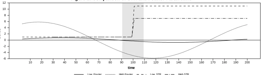
Figure-1 displays the different forms of the smooth transition and the Fourier function,
which we use in the power analysis. A high Fourier form parameter is observed to be in the
range of a relatively low STR function. This indicates that if we use high values of the Fourier
function, it will dominate the sharp break, and the form of the high speed slope parameter of
the smooth transition cannot be sustained in the DGP. Therefore, we use relatively small
values ofαkandβk, which measure the amplitude and displacement of the sinusoidal
component of the deterministic term in the Fourier function. The Fourier function only
mimics the smooth breaks with a single cumulative function; hence, it is better to choose the
Fourier function to detect smooth breaks. The STR model can easily imitate TAR type of
behaviour as well as smooth breaks depending on γ transition speed.
Table-3 shows that our proposed test has significant superiority in all of the parameter
regions. For sharp breaks, we usethe logistic function, whichcan easily capture sharp breaks;
hence, the most important parameters for sharp breaks are γ gamma and intercept parameter
2
α . For the slope parameter, we use the relatively fast transitions of 5.0 and 10.0. Therefore,
as in Figure-1, we obtain moderate and very high speeds of transition from one intercept to
another, which leads to moderate and high sharp breaks. For high break parameterα2, we use
10 and 20, which seem to be sufficient for the second intercept parameter. For the smooth
[image:18.595.87.505.85.205.2]break parameters, we use the Fourier function; αk and βk measure the amplitude and
Figure 1: Comparison of STR and Fourier Parameters
Low Fourier High Fourier Low STR High STR
time
S
e
ri
e
s
10 20 30 40 50 60 70 80 90 100 110 120 130 140 150 160 170 180 190 200 -6
displacement of the sinusoidal component of the deterministic term. Therefore, to prevent the
domination of the Fourier function parameters, we give low values to a low sharp break and
high values to a high sharp break.11 Asmentioned above, one of the most important
parameters in DGP is the speed of transition (gamma, γ ). Therefore, we explain the effects of
gamma in the power simulation study. When gamma increases from 5 to 10, our newly
proposed test gains power in all parameter settings, which shows us that the test works better
in sharp break cases. We seesimilar effects in the LNV test, whereas the EL test behaves
oppositely. For the second important parameter interceptα2, we see that our newly proposed
test and the LNV test are not affected too much; however, the EL test totally loses its power
when it increases from 10 to 20. For threshold location parameter τ, we see that the
magnitude of the power properties of the newly proposed test changes depending on Fourier
parameters αk and βk. When the magnitude of αk and βk is low, changing the break point
from the beginning of the sample to the middle decreases the power of the test and vice versa.
Moreover, increasing the magnitude of αk and βk leads to a power decline in the newly
proposed test; however, the power loss of this parameter change is vast in the LNV model. In
contrast, in this modelling structure, the Fourier form of the unit root testing does not appear
to be a competitor without using cumulative n forms. However, as noted in the introduction,
using the cumulated frequency has some drawbacks, as extensively explained in Becker et al.
(2006) and Enders and Lee (2012a, b).
Table-3: The Power Comparison of Alternative Tests: FKSS DGP with KSS 1stµ
K
k
α βk τ γ α2 sτα τDF C_ sα sτα τDF C_ sα
T=100 T=200
1.0 0.30 0.0 0.5 10.0 10.0 0.289 0.017 0.261 0.723 0.072 0.721 1.0 0.30 0.10 0.5 10.0 10.0 0.301 0.012 0.257 0.774 0.087 0.689 1.0 0.0 0.10 0.5 10.0 10.0 0.383 0.010 0.311 0.839 0.088 0.823
1.0 0.70 0.30 0.5 10.0 10.0 0.160 0.025 0.080 0.451 0.087 0.125 1.0 0.30 0.70 0.5 10.0 10.0 0.137 0.050 0.007 0.335 0.102 0.042 1.0 0.0 0.70 0.5 10.0 10.0 0.157 0.057 0.005 0.358 0.062 0.037 1.0 0.30 0.0 0.2 10.0 10.0 0.347 0.002 0.100 0.952 0.002 0.585 1.0 0.30 0.10 0.2 10.0 10.0 0.329 0.002 0.092 0.964 0.002 0.629 1.0 0.0 0.10 0.2 10.0 10.0 0.395 0.002 0.281 0.972 0.002 0.945 1.0 0.70 0.30 0.2 10.0 10.0 0.127 0.002 0.002 0.596 0.005 0.002 1.0 0.30 0.70 0.2 10.0 10.0 0.077 0.002 0.005 0.506 0.012 0.057 1.0 0.0 0.70 0.2 10.0 10.0 0.140 0.002 0.005 0.538 0.020 0.100 1.0 0.30 0.0 0.5 5.0 10.0 0.269 0.022 0.265 0.929 0.137 0.925 1.0 0.30 0.10 0.5 5.0 10.0 0.255 0.007 0.234 0.881 0.185 0.861 1.0 0.0 0.10 0.5 5.0 10.0 0.317 0.017 0.253 0.937 0.132 0.915 1.0 0.70 0.30 0.5 5.0 10.0 0.122 0.017 0.065 0.669 0.233 0.355 1.0 0.30 0.70 0.5 5.0 10.0 0.105 0.075 0.005 0.413 0.378 0.035 1.0 0.0 0.70 0.5 5.0 10.0 0.157 0.082 0.007 0.438 0.384 0.025 1.0 0.30 0.0 0.2 5.0 10.0 0.323 0.002 0.072 0.957 0.002 0.571 1.0 0.30 0.10 0.2 5.0 10.0 0.301 0.002 0.110 0.943 0.002 0.661 1.0 0.0 0.10 0.2 5.0 10.0 0.341 0.002 0.240 0.969 0.002 0.929 1.0 0.70 0.30 0.2 5.0 10.0 0.137 0.005 0.007 0.604 0.005 0.005 1.0 0.30 0.70 0.2 5.0 10.0 0.097 0.005 0.007 0.453 0.012 0.057 1.0 0.0 0.70 0.2 5.0 10.0 0.152 0.005 0.022 0.571 0.012 0.120 1.0 0.30 0.0 0.5 10.0 20.0 0.257 0.001 0.255 0.761 0.001 0.759 1.0 0.30 0.10 0.5 10.0 20.0 0.281 0.001 0.244 0.751 0.001 0.702 1.0 0.0 0.10 0.5 10.0 20.0 0.321 0.001 0.234 0.844 0.001 0.812 1.0 0.70 0.30 0.5 10.0 20.0 0.125 0.001 0.062 0.488 0.001 0.109 1.0 0.30 0.70 0.5 10.0 20.0 0.426 0.001 0.002 0.842 0.001 0.003 1.0 0.0 0.70 0.5 10.0 20.0 0.523 0.001 0.002 0.876 0.001 0.007 1.0 0.30 0.0 0.2 10.0 20.0 0.357 0.001 0.092 0.929 0.001 0.583 1.0 0.30 0.10 0.2 10.0 20.0 0.307 0.001 0.090 0.935 0.001 0.607 1.0 0.0 0.10 0.2 10.0 20.0 0.361 0.001 0.222 0.963 0.001 0.913 1.0 0.70 0.30 0.2 10.0 20.0 0.182 0.001 0.002 0.747 0.001 0.015 1.0 0.30 0.70 0.2 10.0 20.0 0.087 0.001 0.002 0.610 0.001 0.022 1.0 0.0 0.70 0.2 10.0 20.0 0.165 0.001 0.005 0.807 0.001 0.015 1.0 0.30 0.0 0.5 5.0 20.0 0.297 0.001 0.259 0.901 0.001 0.899 1.0 0.30 0.10 0.5 5.0 20.0 0.249 0.001 0.232 0.913 0.001 0.901 1.0 0.0 0.10 0.5 5.0 20.0 0.305 0.001 0.246 0.947 0.001 0.919 1.0 0.70 0.30 0.5 5.0 20.0 0.117 0.001 0.057 0.650 0.001 0.294 1.0 0.30 0.70 0.5 5.0 20.0 0.421 0.001 0.005 0.946 0.001 0.002 1.0 0.0 0.70 0.5 5.0 20.0 0.518 0.001 0.002 0.972 0.001 0.005 1.0 0.30 0.0 0.2 5.0 20.0 0.305 0.001 0.080 0.949 0.001 0.621 1.0 0.30 0.10 0.2 5.0 20.0 0.351 0.001 0.100 0.941 0.001 0.639 1.0 0.0 0.10 0.2 5.0 20.0 0.375 0.001 0.295 0.951 0.001 0.917 1.0 0.70 0.30 0.2 5.0 20.0 0.165 0.001 0.002 0.714 0.001 0.007 1.0 0.30 0.70 0.2 5.0 20.0 0.112 0.001 0.007 0.627 0.001 0.016 1.0 0.0 0.70 0.2 5.0 20.0 0.152 0.001 0.007 0.781 0.001 0.019
Note:
s
τ
α,τ
DF C_ , ands
αindicate the newly proposed intercept-only test, the Enders and Lee (2012b)4. Empirical results of renewable energy consumption
We use data from 9 countries with available data covering the longest time span:
Canada 1800-2008, France 1800-2008, Germany 1815-2008, Italy 1861-2008, the
Netherlands, 1800-2008, Portugal 1856-2008, Spain 1850-2008, Sweden 1800-2008, and the
UK 1800-2008. Because these 208 years of data may include different types of structures,
such as smooth and sharp breaks, we use different structural break unit root tests to examine
whether renewable energy consumption contains unit root problem. The data source is
updated from Warde, Paul, Energy Consumption in England & Wales, 1560-2004 (Naples:
CNR, 2007).
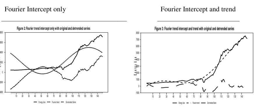
Fourier Intercept only Fourier Intercept and trend
Figure-2 and 3 Fourier Function with Intercept and trend for Italy
As observed in Table-4 and 5, the newly proposed test performs better than the traditionally
used LNV and EL tests used in studies on structural break unit root tests. The newly proposed
test rejects the null hypothesis of unit root with respect to alternative hypothesis of nonlinear
and stationary around simultaneously changing sharp and smooth trend process in all
countries at level with Models A and C only. As mentioned before, the LNV test also captures
the sharp and smooth breaks. Therefore, we expect better performance; however, out of 9
[image:21.595.87.523.338.523.2]Energy Use Fourier trend De-trended Serie
Figure 2: Fourier trend intercept only with original and detrended series
E n e rg y U s e
10 20 30 40 50 60 70 80 90 100 110 120 130 140 -4000 -2000 0 2000 4000 6000
8000 Figure 3: Fourier trend intercept and trend with original and detrended series
Energy Use Fourier trend De-trended Serie
E n e rg y U s e
series, only 4 reject the null hypothesis, again in Models A and C. For the EL test using
Fourier methodology, the intercept-only test performs worst as renewable energy
consumption is historical data with a sharp trend. However, the intercept and trend cases of
the Fourier approach rejectthe null of unit root in two cases. Still, the EL test with the
intercept and trend cannot capture the data-generating process of the historical energy use
data. As mentioned, the Fourier approach only works in smooth breaks if we do not use the
cumulative frequency, and using the cumulative frequency leads to over-filtering the data.
Thus, the Fourier approach with this information is the worst performing test under renewable
energy consumption DGP.
Table-4: Alternative Break Type of Unit Root Tests
LNV test EL
Model A Model B Model C Intercept Int-Trend
Canada -2.777 -2.474 -5.060 -2.079 -2.303
England -2.755 -3.308 -3.093 -0.901 -3.239
France -3.463 -3.059 -5.086 -0.137 -2.855
Germany -3.241 -2.663 -2.812 -1.492 -2.952
Italy -4.107 -3.120 -5.794 -1.089 -1.762
Netherlands -3.848 -2.914 -3.462 0.035 -2.929
Portugal -2.334 -2.470 -3.125 0.975 -2.488
Spain -3.992 -3.455 -4.369 0.777 -3.632
Sweden -3.513 -3.011 -3.593 -0.848 -2.229
Note: LNV Model A, 10%, 3.851, 3.909. LNV Model B, 10%, 4.427, 4.337. LNV Model C, 10%, 4.697, -4.572. For the Enders and Lee (2012 b) EL test, Fourier k=1 and 2, 10% critical values are -3.47 and -2.92 for T = 200.
Table-5: Newly Proposed Test
Model A Model B Model C Model A*
Canada -3.952 -1.687 k=1 lg=1 -5.722 k=2 lg=1 -3.952 k=1 lg=1
England -4.161 -4.785 k=3 lg=1 -4.360 k=3 lg=1 -4.161 k=2 lg=1
France -3.534 -3.226 k=2 lg=3 -5.379 k=2 lg=1 -3.519 k=3 lg=3
Germany -4.056 -2.913 k=1 lg=1 -4.049 k=3 lg=1 -4.047 k=3 lg=1
Italy -3.565 -2.893 k=2 lg=1 -5.327 k=4 lg=8 -3.565 k=4 lg=1
Netherland -5.176 -4.260 k=2 lg=1 -5.835 k=4 lg=1 -5.176 k=1 lg=1
Portugal -4.526 -2.737 k=2 lg=1 -3.359 k=3 lg=1 -4.526 k=1 lg=1
Spain -5.068 -4.535 k=2 lg=5 -4.532 k=4 lg=1 -4.186 k=4 lg=5
Sweden -4.460 -3.011 k=2 lg=1 -3.718 k=4 lg=1 -4.460 k=1 lg=1
Moreover, our methodology clearly identifies sharp and smooth breaks in renewable
energy consumption historical data. For Germany, the Netherlands, Portugal and Sweden,
other tests conclude as a unit root process i.e. renewable energy consumption is nonstationary
at level. However, our newly proposed test clearly identifies stationary process in renewable
energy consumption at level with 1 sharp and 3 smooth breaks for Germany, 1 sharp and 4
smooth breaks for the Netherlands with Model C, 1 sharp and 1 smooth break for Portugal
and, 1 sharp and 1 smooth break for Sweden. This data structure is not that easy to capture
with a simple unit root test procedure. Therefore, we can conclude that tests which do not
consider the general data structure may lead to a misspecified model, and the results obtained
from these models may be misleading.
Table-6: Parameter Values Obtained for Model A
Lag order K
2
α
τ
γ
α
kCanada lg=1 k=1 13811.02 0.867 0.053 -0.391
England lg=1 k=2 16145.45 0.529 0.011 -63.784
France lg=3 k=3 10209.34 0.844 0.033 4.447
Germany lg=1 k=3 17336.86 0.692 0.026 50.355
Italy lg=1 k=4 6458.48 0.738 0.108 -37.219
Netherland lg=1 k=1 3178.707 0.826 0.069 -3.464
Portugal lg=1 k=1 1888.655 0.969 0.057 -1.334
Spain lg=4 k=4 8950.105 0.984 0.051 7.934
Sweden lg=1 k=1 1494.338 0.765 0.069 -1.163
Average - 2 8830.32 0.801 0.053 -4.957
Panel B- Empirical Power Analysis Depending on Parameter Values
ρ
2
α
τ
γ
α
ks
τ
ατ
DF C_s
α0.8 8830.3 0.801 0.053 -4.957 0,982 0,003 0,907
0.2 8830.3 0.801 0.053 -4.957 0,942 0,003 0,805
Note: ρ for the first row of Panel B we choose the high persistency parameter like in the power analysis the second one is obtained from the empirical analysis which shows low persistence.
We note that Table 6 panel A, provides information of nonlinear parameters from
Model A. These parameters indicate that there is a very sharp break in the end of samples for
this mean in the beginning of ¾ sample period. On the other hand, break parameter is very
high i.e. α2=8830.3with average sharp breaks for 9 countries. The gamma parameter indicates
that average transition speed between these two means (low and high mean values) is slow i.e.
0.053
γ = . Finally, Fourier parameters are estimated to be relatively small with respect to
break parameterα2. In panel B of Table 6, we have used these average parameter values to
detect whether newly proposed test well perform under these parameter values. The results
obtained in Table 6 from the empirical power analysis indicate the similar conclusion with
unit root test results given in Table-4 and 5. Moreover, the empirical power results are also
consistent with the power analysis which is given in Table-2. The first best test in this
parameter region is newly proposed test i.e. SOR unit root test and second best test is LNV
unit root test and finally the Fourier type of unit root test namely EL has nearly no power with
these parameter values. Shortly, renewable energy consumption data with these results or
parameter values obtained in panel A of Table-6 includes a sharp break which can be captured
by logistic smooth transition function and multiple smooth breaks that can be detected by
Fourier function. Therefore, testing procedure for the longer period renewable energy
consumption data must contain simultaneously these two features. The LNV unit root test
only includes the logistic transition function in its testing procedure and EL unit root test
Fourier function, hence, these tests make mis-specification error while testing the long span
renewable energy consumption stationary properties.
Step 3 STR-Fourier Trend Comparison of OS and LNV trends
Figure-4, 5, 6 and 7 for Italy data; STR trend; Fourier trend obtained from residuals of STR
trend STR + Fourier (SOR trend); comparison of STR and SOR trend
5. Conclusion and Policy Implications
This study proposed a flexible unit root test that detects sharp and smooth breaks
simultaneously in time series data. Most of the unit root tests are not general enough to
capture different dynamics, such as smooth structural breaks, sharp structural breaks, state
dependent-nonlinearity or a mixture of them. Therefore, considering all these data structures
in one unit root process is important, and the results produced by this type of test structure do
not face misspecification problems. We test stationary properties for 9 countries’ historical
renewable energy consumption data covering the 1800-2008 period with traditionally used
structural break unit root tests and a newly proposed test. The newly proposed unit root test
[image:25.595.79.497.68.410.2]performs better than the traditional ones. The empirical results by SOR unit root test show the
Figure 4:ST trend with original and detrended series
Energy Use ST trend de-trended serie
E n e rg y U s e
[image:25.595.309.497.79.203.2]10 20 30 40 50 60 70 80 90 100 110 120 130 140 -1000 0 1000 2000 3000 4000 5000 6000 7000 8000
Figure 5: Fourier trend with original and detrended series
Energy Use Forier trend detrended Series
E n e rg y U s e
10 20 30 40 50 60 70 80 90 100 110 120 130 140 -750 -500 -250 0 250 500 750
Figure 6: SOR trend with original and detrended series
OS trend detrended Series Energy Use detrended Series
E n e rg y U s e
10 20 30 40 50 60 70 80 90 100 110 120 130 140 -1000 0 1000 2000 3000 4000 5000 6000 7000 8000
Figure 7: SOR and ST trend with original and detrended series
OS trend ST trend Energy Use
E n e rg y U s e
Tests of the time-series stationary properties of renewable energy consumption have many
implications for the design of energy policy. For example, as mentioned before, if energy
consumption follows a stationary process, then shocks to the global energy market will have a
temporary or transitory effect on renewable energy consumption. In such circumstances,
shocks to energy consumption will result in temporary deviation from the long-run path, and
thus, renewable energy consumption returns to its trend path after a certain time. This
suggests that governments should avoid the unnecessary adoption of energy targets as
renewable energy consumption deviates from long-run path temporarily. In such a situation,
the implementation of energy conservation and energy management policies for reducing
energy intensity or consumption is meaningless over a long time span. Therefore, our test
procedure is the best indicator for policy makers to see the long-run trends and the deviation
from this long-run path. The true data generating process of long span renewable energy
consumption has two important components: a sharp break and more than one smooth breaks
around this sharp break. This means that correctly specified models must include these feature
of renewable energy consumption data while testing or estimating renewable energy demand.
Any other modelling can lead to wrong results which in turn, misleads the policy makers to
adapt appropriate energy policies. Thus, correct polices can be implemented only by using
References
Apergis, N., Loomis, D. and Payne, J. E., 2010. Are shocks to natural gas consumption
temporary or permanent? Evidence from a panel of U.S. states. Energ Policy 38,
4734-4736.
Apergis, N. and Payne, J. E., 2010. Structural breaks and petroleum consumption in US states:
Are shocks transitory or permanent? Energ Policy 38, 6375-6378.
Aslan, A., 2011. Does natural gas consumption follow a nonlinear path over time? Evidence
from 50 US states. Renewable and Sustainable Energy Reviews 15, 4466-4469.
Aslan, A. and Kum, H., 2011. The stationary of energy consumption for Turkish disaggregate
data by employing linear and nonlinear unit root tests. Energy 36, 4256-4258.
Barros, C. P., Gil-Alana, L. A. and Payne, J. E., 2013. U.S. Disaggregated renewable energy
consumption: persistence and long memory behavior. Energy Economics 40, 425-432.
Becker, R., Enders. W. and Lee, J., 2006. A stationarity test in the presence of an unknown
number of smooth breaks. Journal of Time Series Analysis 27, 381-409.
Bolat, S., Belke, M. and Celik, N., 2013. Mean reverting behavior of energy consumption:
evidence from selected MENA countries. International Journal of Energy Economics
and Policy 3, 315-320.
Breuer, J. B., McNown, R. and Wallace, M. S., 2001. Misleading inferences from panel
unit-root tests with an illustration from purchasing power parity. Review of International
Economics 9, 482-493.
Carrion i Silvestre, J. L., Sansó i Rosselló, A. and Artís Ortuño, M., 1999. Response surfaces
estimates for the Dickey-Fuller unit root test with structural breaks. Economics Letters
63, 279-283.
Chen, P. F. and Lee, C. C., 2007. Is energy consumption per capita broken stationary? New
Davies, R. B., 1987. Hypothesis testing when nuisance parameters is only identified under the
alternative. Biometrika, 47, 33-43.
Demir, E. and Gozgor, G. (2017). Are shocks to renewable energy consumption permanent
or temporary? Evidence from 54 developing and developed countries. Environmental
Science and Pollution Research, 1-8.
Dornbusch, R., 1976. Expectations and exchange rate dynamics. Journal of Political Economy
84, 1161-1176.
Enders, W. and Lee. J., 2012. A unit root test using a Fourier series to approximate smooth
breaks. Oxford Bulletin of Economics and Statistics, 74(4), 574-599.
Granger, C. W. J., 1969. Investigating causal relations by econometric models and
cross-spectral methods. Econometrica 37, 424-438.
Hamilton, J. D., 1996. This is what happened to the oil price-macroeconomy relationship.
Journal of Monetary Economics 38, 215-220.
Hasanov, M. and Telatar, E., 2011. A re-examination of stationarity of energy consumption:
evidence from new unit root tests. Energy Policy 39, 7726-7738.
Hendry, D. F. and Juselius, K., 2000. Explaining cointgeration analysis. Energy Journal 21,
1-42.
Hsu, Y. C., Lee, C. C. and Lee, C. C., 2008. Revisited: are shocks to energy consumption
permanent or temporary? New evidence from a panel SURADF approach. Energy
Economics 30, 2314-2330.
Im, K.S., Pesaran, M.H., Shin, Y., 2003. Testing for unit roots in heterogeneous panels.
Journal of Econometrics 115, 53-74.
Johansen, S. and Juselius, K., 1990. Maximum likelihood estimation and inference on
cointegration with applications to the demand for money. Oxford Bulletin of Economics
Kapetanios, G., Shin, Y. and Snell, A., 2003. Testing for a unit root in the nonlinear STAR
framework. Journal of Econometrics 112, 359-379.
Kula, F., Aslan, A. and Ozturk, I., 2012. Is per capita electricity consumption stationary?
Time series evidence from OECD countries. Renewable and Sustainable Energy Review
16, 501-503.
Kum, H., 2012. Are fluctuations in energy consumption transitory or permanent? Evidence
from a panel of East Asia & Pacific countries. International Journal of Energy
Economics and Policy 2, 92-96.
Lean, H. H. and Smyth, R., 2014. Are shocks to disaggregated energy consumption in
Malaysia permanent or temporary? Evidence from LM unit root tests with structural
breaks. Renewable and Sustainable Energy Review 31, 319-328.
Lee, C., Wu, J. L. and Yang, L. W, 2016. A simple panel unit-root test with smooth breaks in
the presence of a multifactor error structure. Oxford Bulletin of Economics and Statistics
78, 365-393.
Lee, J. and Strazicich, M. C., 2003. Minimum Lagrange multiplier unit root test with two
structural breaks. Review of Economics and Statistics 85, 1082-1089.
Liu, W.-C., 2013. The study on the stationarity of energy consumption in US states:
considering structural breaks, nonlinearity, and cross-sectional dependency.
International Journal of Mathematical and Computional Scinces 7, 1310-1330.
Magazzino, C., 2017a. Is per capita energy use stationary? Panel data evidence for the EMU
countries. Energy Exploration and Exploitation 35, 24-32.
Magazzino, C., 2017a. Stationarity of electricity series in MENA countries. The Elctricity
Journal, 30, 16-22.
Mishra, V., Sharma, S. and Smyth, R., 2009. Are fluctuations in energy consumption per
Narayan, P.K., Narayan, S. and Popp, S., 2010. Energy consumption at the state level: the unit
root null hypothesis from Australia. Applied Energy 87, 1953-1962.
Narayan, P. K. and Popp, S. (2010). A new unit root test with two structural breaks in level
and slope at unknown time. Journal of Applied Statistics, 37, 1425-1438.
Ng, S. and Perron, P., 2001. Lag length selection and the construction of unit root tests with
good size and power. Econometrica 69, 1519-1554.
Oh, W. and Lee, K., 2004. Causal relationship between energy consumption and GDP
revisited: the case of Korea 1970–1999. Energy Economics 26, 51-59.
Omay, T., Çorakcı, A. and Emirmahmutoğlu, F., 2017. Real interest rates: nonlinearity and
structural breaks. Empirical Economics 52, 283-307.
Omay, T., Emirmahmutoglu, F. and Hasanov, M., 2017. Structural break, nonlinearity and
asymmetry: a re-examination of PPP proposition. Applied Economics, 1–20.
Omay, T. and Emirmahmutoğlu, F., 2017. The comparison of power and optimization
algorithms on unit root testing with smooth transition. Computional Economics 49,
623-651.
Omay, T., Hasanov, M. and Shin, Y., 2018. Testing for unit roots in dynamic panels with
smooth breaks and cross-sectionally dependent errors. Computional Economics. doi:
10.1007/s10614-017-9667-7.
Ozcan, B., 2013. Are shocks to energy consumption permanent or temporary? The case of 17
Middle East countries. Energy Exploration and Exploitation 31, 589-605.
Ozcan, B. and Ozturk, I., 2016. A new approach to energy consumption per capita
stationarity: evidence from OECD countries. Renewable and Sustainable Energy
Review 65, 332-344.
Ozturk, I. And Aslan, A., 2011. Are fluctuations in energy consumption per capita transitory?
Sadorsky, P., 1999. Oil price shocks and stock market activity. Energy Economics 21,
449-469.
Schmidt, P., Phillips, P.C.B., 1992. LM tests for a unit root in the presence of deterministic
trends. Oxford Bulletin of Economics and Statistics 54, 257287.
Shahbaz, M., Hoang, T. H. V., Mahalik, M. K. and Roubaud, D., 2017. Energy consumption,
financial development and economic growth in India: new evidence from a nonlinear
and asymmetric analysis. Energy Economics 63, 199-212.
Shahbaz, M., Khraief, N., Mahalık, M. K. and Zaman, K. U., 2014. Are fluctuations in natural
gas consumption per capita transitory? Evidence from time series and panel unit root
tests. Energy 78, 183-195.
Shahbaz, M., Kumar Tiwari, A.K., Ozturk, I. And Farooq, A., 2013. Are fluctuations in
electricity consumption per capita transitory? Evidence from developed and developing
economies. Renewable and Sustainable Energy Review 28, 551-554.
Shahbaz, M., Solarin, S. A. and Mallick, H., 2015. Are fluctuations in gas consumption per
capita transitory? Evidence from LM unit root test with two structural breaks. Bulletin
of Energy Economics 3, 203-209.
Shahbaz, M., Tiwari, A. K. and Khan, S., 2016. Is energy consumption per capita stationary?
Evidence from first and second generation panel unit root tests. Economics Bulletin 36,
1656-1669.
Smyth, R., 2013. Are fluctuations in energy variables permanent or transitory? A survey of
the literature on the integration properties of energy consumption and production.
Applied Energy 104, 371-378.
Taylor, J., 1979. Staggered wage setting in a macro model. American Economic Review 69,
Ucar, N. and Omay, T., 2009. Testing for unit root in nonlinear heterogeneous panels.
Economics Letters 104, 5-8.
Wang, Y., Li, L., Kubota, J., Zhu, X. and Lu, G., 2016. Are fluctuations in Japan’s
consumption of non-fossil energy permanent or transitory? Applied Energy 169,
187-196.
Yilanci, V. and Tunali, Ç. B., 2014. Are fluctuations in energy consumption transitory or
permanent? Evidence from a Fourier LM unit root test. Renewable and Sustainable
Appendix A1.
Figures of the rest of de-trending strategies for Italy data
Model B of Italy
Model C of Italy
[image:33.595.74.525.200.725.2]Energy Use ST trend detrended Series
Figure 1:ST trend with original and detrended series
E n e re g y U s e
10 20 30 40 50 60 70 80 90 100 110 120 130 140 -1200 0 1200 2400 3600 4800 6000 7200 8400
Energy Use Forier trend detrended Series
Figure 2: Fourier trend with original and detrended series
E n e re g y U s e
10 20 30 40 50 60 70 80 90 100 110 120 130 140 -1200 -800 -400 0 400 800 1200
OS trend detrended Series Energy Use detrended Series
Figure 3: OS trend with original and detrended series
E n e re g y U s e
10 20 30 40 50 60 70 80 90 100 110 120 130 140 -1200 0 1200 2400 3600 4800 6000 7200 8400
OS trend ST trend Energy Use
Figure 4: OS and ST trend with original and detrended series
E n e re g y U s e
10 20 30 40 50 60 70 80 90 100 110 120 130 140 -1200 0 1200 2400 3600 4800 6000 7200 8400
Energy Use ST trend detrended Series
Figure 1:ST trend with original and detrended series
E n e re g y U s e
10 20 30 40 50 60 70 80 90 100 110 120 130 140 -1000 0 1000 2000 3000 4000 5000 6000 7000 8000
Energy Use Forier trend detrended Series
Figure 2: Fourier trend with original and detrended series
E n e re g y U s e
Model A* Italy
[image:34.595.83.522.68.608.2]OS trend detrended Series Energy Use detrended Series
Figure 3: OS trend with original and detrended series
E n e re g y U s e
10 20 30 40 50 60 70 80 90 100 110 120 130 140 -1000 0 1000 2000 3000 4000 5000 6000 7000 8000
OS trend ST trend Energy Use
Figure 4: OS and ST trend with original and detrended series
E n e re g y U s e
10 20 30 40 50 60 70 80 90 100 110 120 130 140 0 1000 2000 3000 4000 5000 6000 7000 8000
Energy Use ST trend detrended Series
Figure 1:ST trend with original and detrended series
E n e re g y U s e
10 20 30 40 50 60 70 80 90 100 110 120 130 140 -1000 0 1000 2000 3000 4000 5000 6000 7000 8000
Energy Use Forier trend detrended Series
Figure 2: Fourier trend with original and detrended series
E n e re g y U s e
10 20 30 40 50 60 70 80 90 100 110 120 130 140 -750 -500 -250 0 250 500 750
OS trend detrended Series Energy Use detrended Series
Figure 3: OS trend with original and detrended series
E n e re g y U s e
10 20 30 40 50 60 70 80 90 100 110 120 130 140 -1000 0 1000 2000 3000 4000 5000 6000 7000 8000
OS trend ST trend Energy Use
Figure 4: OS and ST trend with original and detrended series
E n e re g y U s e
Appendix A2.
Critical values of Model A*
*
α
τ
s
T 1% 5% 10%
k=1
25 -5.925 -4.957 -4.529
50 -5.415 -4.740 -4.408
100 -5.171 -4.566 -4.245
200 -4.970 -4.501 -4.249
500 -4.973 -4.485 -4.241
k=2
25 -5.923 -5.019 -4.609
50 -5.361 -4.794 -4.450
100 -5.310 -4.590 -4.329
200 -5.149 -4.581 -4.258
500 -5.125 -4.541 -4.218
k=3
25 -6.264 -5.063 -4.614
50 -5.405 -4.597 -4.216
100 -5.338 -4.629 -4.242
200 -5.227 -4.576 -4.267
500 -5.136 -4.510 -4.204
k=4
25 -5.840 -4.772 -4.191
50 -5.358 -4.585 -4.180
100 -5.321 -4.464 -4.150
200 -5.071 -4.387 -4.148
500 -4.880 -4.403 -4.113
k=5
25 -5.449 -4.454 -3.980
50 -5.219 -4.505 -4.096
100 -5.067 -4.426 -4.083
200 -4.987 -4.357 -4.040
Appendix A3.
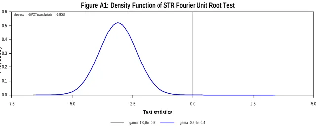
Density functions of the STR-Fourier-type t-statistics and their invariance properties.
Leybourne et al. (1998) showed that the analytical demonstration of the invariance
property is difficult under the proposed detrending methods. They made the following
modification: As the NLS estimation of parameters γ and τ does not concede closed-form
explanations, it would be enormously problematic to consequently create any analytical
association between the v andˆ yt. This makes the determination of the null