Application of Self-Tuning Control System for Solution of Fault Tolerance Problem

Application of Self-Tuning Control System for

Solution of Fault Tolerance Problem

Yuri A. Vershinin, Member, IAENG

Abstract - Self-tuning control can provide desirable behaviour of a process even though the process parameters are unknown or may vary with time. Conventional self-tuning control requires that the speed of adaptation must be more rapid than that of the parameter changes. However, in practice, problems do arise when this is not the case. For example, when fault occurs in a process, the parameters may change very dramatically. A new approach based on simultaneous identification and adaptation of unknown parameters is suggested for compensation of rapidly changing parameters. High dynamic precision self-tuning control can be used for the solution of a fault tolerance problem in complex and multivariable processes and systems.

Index Terms - Self-tuning control, identification, fault tolerance, Singular Value Decomposition.

I. DETERMINATION OF A MATHEMATICAL MODEL OF A PROCESS

A mathematical model of a process on a stationary regime can be found from the sequence of Markov parameters using the classical Ho algorithm [1]. The Markov parameters can be obtained from input – output relationships or more directly as an impulse response of the system. It is well known that according to the theorem of Kronecker the rank of the Hankel matrix constructed from the Markov parameters is equal to the order of the system from which the parameters are obtained. Therefore, by consistently increasing the dimension of the Hankel matrix

 until

rank r = rank r1

the order of the system can be obtained as equal to r. However, in practical implementation, this rank – order relationship may not give accurate results due to several factors: sensitivity of the numerical rank calculation and bias of the rank if information about the process is corrupted by noise. This problem can be avoided using singular value decomposition (SVD) of the Hankel matrix:

T

USV



 ₍₁₎

Manuscript received June 28, 2012; revised August 08, 2012.

Yuri A. Vershinin is Senior Lecturer and Director of Intelligent Transport Systems and Telematics Applied Research Group, Department of Mechanical and Automotive Engineering, Coventry University, UK, (email: [email protected]).

where

I V V U

UT  T  _,

) ... , ,..., ,

( _{1 2 l l 1, n}

diag

S      _  _.

Here U and V are orthogonal matrices. The diagonal elements of the matrix S (the singular values) in (1) are arranged in the following order 12 ...n 0. Applying the property of SVD to reflect the order of a system through the smallest singular value, the order of the system can be determined with the tolerance required. From practical point of view a reduced order model is more preferable. Taking into account that the best approximation in the Hankel norm sense is within a distance of l1, the

model of order l can be found. However, a relevant matrix built from Markov parameters of this reduced order model should also be of the Hankel matrix. But it is not an easy matter to find such a Hankel matrix for the reduced order process. A simpler solution, although theoretically not the best, can be found from the least squares approximation of the original Hankel matrix [2], [3] and [4]. The discrete time state space realisation of the process can be determined from the relationship between Markov parameters and representation of the Hankel matrix through relevant controllability and observability matrices of the process:

2 2

. . .

. d

d d

d d d d d

d d

C C A

A A B A B

C A

 

 

 

   

  _{ } 

 

 

 

 

(2)

where d

A _{is the system matrix,}

d

B _{is the control matrix,}

d

C _{is the output matrix,}

 _{is the observability matrix,}  _{is the controllability matrix.}

II. THE SELF-TUNING CONTROL SYSTEM Consider a continuous time single input – single output second order plant (a process) given in the following canonical state space realisation form:

x C y

u B x A x

c c c 

  

where        p p c a a A 2 1 1 0 ,        1 0 c

B _, Cc  c1p c2p ,

u _{is the control signal,} y _{is the output of the plant.}

Assume that at the time t parameters a1p and a2p change dramatically due to a fault in the system, but parameters

p

c_{1 and} c_{2p remain constant. The mathematical model of}

plant (3) can be represented in the following form:

p p p p p p p p p p p p x c x c y u x t a a x t a a x 1 2 1 1 2

2 ()) ( ())

(              where ) ( 1 1

1 a a t

a _p  _p _{p ,}

) ( 2 2

2 a a t

a p  p p , p p p p a c c

a₁ , ₂ , ₁ , ₂ are the nominal parameters (constant) of the plant,

), (

1 t a _p

 a_2p(t) are the biases of the plant parameters (variable) from their nominal values,

p

x is the plant state, p

y is the plant output.

A desirable behaviour of the plant can be determined by the following reference model:

m m m m m m m m m m x c x c y g x a x a x 1 2 1 2         

, ₍₄₎

where

g _{is the input signal,}

m

a_{1 ,} a_2m, c_1m, c_{2m are parameters of the model.}

In order to compensate for the plant parameters' biases, a controller can be used. The closed loop system with the controller is represented in the following form:

p p p p p p

p a a t x a a t x

x ( ₂  ₂ ()) ( ₁  ₁ ())

g x t k k x t k

k  _p   _p

( _{2 2}()) ( _{1 1}()) (5)

where ,

1

k k₂ are the constant parameters of the controller,

) ( 1 t

k

 , k₂(t) are the adjustable parameters of the controller.

The desirable quality of the process behaviour can be obtained from the following relationships:

m p a

a k1 1  1

m p a

a

k₂ ₂  ₂ .

According to equations (4) and (5), the error equation is obtained as follows:

p p m

me a e z x z x

a

e ₂  ₁  ₂  ₁ , (6)

where:

p m x

x

e  ,

) ( )

( ₁

1

1 a t k t

z  _p  ,

) ( )

( ₂

2

2 a t k t

z  _p  .

It can be seen from equation (6) that in order to achieve the desirable error e0, it is necessary to provide the following conditions:

0 1

z , z2 0. (7)

The conditions (7) can be achieved by adjusting parameters

) ( 1 t

k

 and k2(t) according to the following laws [5]:

p

x t k 

₁() (8)

p

x t k 

 ₂( ) , where Pe.

The positive definite symmetric matrix P can be obtained from the solution of the relevant Lyapunov equation. The main problem associated with algorithms (8) is that all self-tuning contours are linked through the dynamics of the plant. The consequence is that high interaction of each contour with others will occur. This further results in poor dynamic compensation of plant parameters' biases a_ip i

=1,2,…,m, where m is a number of self-tuning contours. The idea of decoupling self-tuning contours from plant dynamics, based on simultaneous identification and adaptation, is suggested for the solution of this problem with fault tolerance. This could considerably improve performance of the overall system, especially for high dimension and multivariable plants and processes.

It can be shown [6], [7] that the self-tuning contours will be decoupled from the plant dynamics if  can be formed such that:

e a e a

e _{2m 1m}

* _{  }

   .

In this case the following relationship can be obtained: 

   

 ( a2p(t) k2(t))xp

*

p p t k t x

a () ( ))

( ₁  ₁ . (9)

In order to solve equation (9) with two variable parameters, the following approach is suggested: Multiply both parts of equation (9) by state variables x_p and x_p and integrate the resultant equations on the time interval (t1,t2), where:

t t

t₂  ₁ . Taking the initial conditions as t₁0,

0









         t t t p p t t t p p p p t t t dt x a dt x x a dt x 1 1 1 1 1 1 2 1 2 * _







         t t t p p p t t t p p p t t t dt x x a dt x a dt x 1 1 1 1 1 1 1 2 2 *_{  } . (10) Introduce the following notations:

1 * 1 1 c dt x_p t t t  



 

, 2

* 1 1 c dt x_p t t t  



   , 11 2 1 1 l dt x t t t p 



 

, 21

1 1 l dt x x t t t p p 



   , 12 1 1 l dt x x _p t t t p 



 

 , 22

2 1 1 l dt x t t t p 



 

 . (11)

According to notations (11), equations (10) can now be written in the form:

22 2 21 1 2 12 2 11 1 1 l a l a c l a l a c p p p p        

. (12)

From the solution of equations (12) the bias of the plant parameters a_ip, (i1,2) can be determined. The controller can be adjusted according to the estimated parameter bias as:

ip

i a

k 

 .

Therefore, conditions (7) are satisfied, which in turn means that the behaviour of system (5) follows the desirable trajectories of model (4), even in the presence of dramatic plant parameters changes.

For the solution of equations (12) one needs to take into account of the hypothesis of quasi-stationarity of the process, where the interval time t is selected such that the biases of parameters a_ip must be constant at this interval. However, the interval t should be sufficiently large in order to accumulate a larger quantity of variables xp and

p

x for the solution of the equations.

III. THE NUMERICAL RESULTS

The Hankel matrix , constructed from the Markov parameters (obtained from the experiment, see APPENDIX), is as follows:

            01 -1.2447038e 01 -1.5056000e 01 -1.6442500e 01 -1.5056000e 01 -1.6442500e 01 -1.4550000e 01 -1.6442500e 01 -1.4550000e 02 -6.5000000e . (13) Applying the singular value decomposition procedure (1) on the Hankel matrix (13), it is found that

           01 -5.7560070e 01 -5.6753434e -01 -5.8871776e 01 -7.7101797e 01 -1.3682059e -01 -6.2194166e 01 -2.7242453e 01 -8.1190203e 01 -5.1633320e U            01 -5.7560070e 01 -5.6753434e 01 -5.8871776e 01 -7.7101797e -01 -1.3682059e 01 -6.2194166e 01 -2.7242453e 01 -8.1190203e -01 -5.1633320e V                  04 -6.1531296e 00 0.0000000e 00 0.0000000e 00 0.0000000e 02 -7.4455532e 00 0.0000000e 00 0.0000000e 00 0.0000000e 01 -4.2773559e S (14)

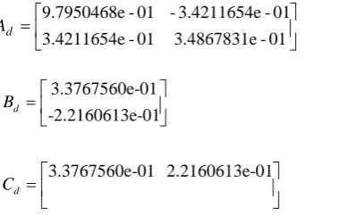
Using relations (1), (2) and (14) the discrete time state space realisation of the reduced order system is obtained as follows:        01 -3.4867831e 01 -3.4211654e 01 -3.4211654e -01 -9.7950468e d A 3.3767560e-01 -2.2160613e-01 3.3767560e-01 2.2160613e-01 d d B C               (15)

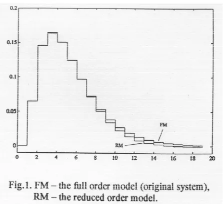
The behaviour of the full order model and the reduced order model is given in Figure 1. It can be seen in Fig. 1 and APENDIX that the Markov parameters of the reduced order model are a close approximation to the Markov parameters of the original system.

Nominal parameters of the plant in the continuous time (3) are obtained from (15) as follows:

1184 . 3

1p 

a _, a_2p 3.0517_, 0318

. 0

1p 

c _, c_2p 2.9132_.

Parameters of model (4) are chosen as a_1ma_1p, p

m a

a₂  ₂ , c_1mc_1p, c_2mc_2p.

[image:3.595.51.287.46.310.2] [image:3.595.310.514.390.511.2]

The performance of the high dynamic precision self-tuning control system are presented in Fig. 2 - 5.

Fig. 3. shows the bias from the nominal parameter at t1

sec. with adaptation being switched on (a_1p 1, 0

2 

a _p ). It can be seen that the output of system p

y coincides with the model reference output ym after t4 sec.

[image:4.595.305.529.381.586.2]

Fig. 4. shows that the bias from the nominal parameter at time t1 sec. is a_2p 1, (a_1p 0). The adaptation is switched off.

Fig. 5. shows the bias from the nominal parameter at t1

sec. with adaptation being switched on (a_2p 1, 0

1 

a _p ). It can be seen that the output of system p

y coincides with the model reference output ym after t9 _sec.

IV. CONCLUSIONS

The high dynamic precision self-tuning control system for the solution of a fault tolerance problem of a SISO process is suggested in this paper. The method, which is based on simultaneous identification and adaptation of unknown process parameters, provides decoupling of self-tuning contours from plant dynamics. The control system compensates the rapidly changing parameter when fault occurs in a process. The mathematical model of the process is formed from Markov parameters, which are obtained from the experiment as the process impulse response. The order of the model is determined using singular value decomposition of the relevant Hankel matrix. This allows one to obtain a robust reduced order model representation if the information about the process is corrupted by noise in industrial environment.

REFERENCES

[1] Ho, B.L.andR.E. Kalman (1966). Effective construction of linear state-variable models from input/output functions. Proceedings The Third Allerton Conference, 449-459.

[2] Zeiger, H.P. and A.J. McEwen (1974). Approximate linear realizations of given dimension via Ho's algorithm. IEEE Transactions on Automatic Control, 19, 153.

[3] Kalman, R.E., P.L. Falb and M.A. Arbib (1974). Topics in Mathematical System Theory. McGraw Hill.

[4] Moor, B.C. (1981). Principal component analysis in linear systems: Controllability, observability and model reduction. IEEE Transactions on Automatic Control, 26, 17 – 32.

[5] Astrom, K.J. and B. Wittenmark (1995). Adaptive Control. Addison – Wesley, Reading, Mass.

[6] Petrov, B.N., V.Y. Rutkovsky and S.D. Zemlyakov (1980). Adaptive coordinate-parametric control of nonstationary plants. Nauka, Moscow.

[7] Vershinin, Y.A. (1991). Guarantee of tuning independence in multivariable systems. Proceedings The Fifth Leningrad Conference on theory of adaptive control systems: "Adaptive and expert systems in control", _Leningrad.

APPENDIX

Markov parameters Markov parameters of obtained from the reduced order the experiment: model: