German Semantic Verb Classes
Sabine Schulte im Walde
∗ Universit¨at des SaarlandesThis article presents clustering experiments on German verbs: A statistical grammar model for German serves as the source for a distributional verb description at the lexical syntax–semantics interface, and the unsupervised clustering algorithm k-means uses the empirical verb properties to perform an automatic induction of verb classes. Various evaluation measures are applied to compare the clustering results to gold standard German semantic verb classes under different criteria. The primary goals of the experiments are (1) to empirically utilize and investigate the well-established relationship between verb meaning and verb behavior within a cluster analysis and (2) to investigate the required technical parameters of a cluster analysis with respect to this specific linguistic task. The clustering methodology is developed on a small-scale verb set and then applied to a larger-scale verb set including 883 German verbs.
1. Motivation
Semantic verb classes generalize over verbs according to their semantic properties, that is, they capture large amounts of verb meaning without defining the idiosyncratic details for each verb. The classes refer to a general semantic level, and idiosyncratic lexical semantic properties of the verbs are either added to the class description or left underspecified. Examples for semantic verb classes arePositionverbs such asliegen ‘lie’,sitzen‘sit’,stehen‘stand’, andManner of Motion with a Vehicleverbs such asfahren ‘drive’, fliegen ‘fly’, rudern ‘row’. Manual definitions of semantic verb classes exist for several languages, the most dominant examples concerning English (Levin 1993; Baker, Fillmore, and Lowe 1998) and Spanish (V´azquez et al. 2000). On the one hand, verb classes reduce redundancy in verb descriptions since they encode the common properties of verbs. On the other hand, verb classes can predict and refine properties of a verb that received insufficient empirical evidence, with reference to verbs in the same class: Under this criterion, a verb classification is especially useful for the pervasive problem of data sparseness in NLP, where little or no knowledge is provided for rare events. For example, the English verb classification by Levin (1993) has been used in NLP applications such as word sense disambiguation (Dorr and Jones 1996), machine translation (Dorr 1997), document classification (Klavans and Kan 1998), and subcat-egorization acquisition (Korhonen 2002). To my knowledge, no comparable German verb classification is available so far; therefore, such a classification would provide a principled basis for filling a gap in available lexical knowledge.
How can we obtain a semantic classification of verbs while avoiding tedious manual definitions of the verbs and the classes? Few resources are semantically annotated and provide semantic information off-the-shelf such as FrameNet (Baker, Fillmore, and Lowe 1998; Fontenelle 2003) andPropBank(Palmer, Gildea, and Kingsbury 2005). Instead, the automatic construction of semantic classes typically benefits from a long-standing linguistic hypothesis that asserts a tight connection between the lexical meaning of a verb and its behavior: To a certain extent, the lexical meaning of a verb determines its behavior, particularly with respect to the choice of its arguments (Pinker 1989; Levin 1993; Dorr and Jones 1996; Siegel and McKeown 2000; Merlo and Stevenson 2001; Schulte im Walde and Brew 2002; Lapata and Brew 2004). Even though the meaning–behavior relationship is not perfect, we can make this prediction: If we induce a verb classification on the basis of verb features describing verb behavior, then the resulting behavior classification should agree with a semantic classification to a certain extent (yet to be determined). The aim of this work is to utilize this prediction for the automatic acquisition of German semantic verb classes.
The verb behavior itself is commonly captured by the diathesis alternation of verbs: alternative constructions at the syntax–semantics interface that express the same or a similar conceptual idea of a verb (Lapata 1999; Schulte im Walde 2000; McCarthy 2001; Merlo and Stevenson 2001; Joanis 2002). Consider example (1), where the most common alternations of theManner of Motion with a Vehicleverbfahren‘drive’ are illustrated. The conceptual participants are a vehicle, a driver, a passenger, and a direction. In (a), the vehicle is expressed as the subject in a transitive verb construction, with a prepositional phrase indicating the direction. In (b), the driver is expressed as the subject in a tran-sitive verb construction, with a prepositional phrase indicating the direction. In (c), the driver is expressed as the subject in a transitive verb construction, with an accusative noun phrase indicating the vehicle. In (d), the driver is expressed as the subject in a ditransitive verb construction, with an accusative noun phrase indicating the passenger, and a prepositional phrase indicating the direction. Even if a certain participant is not realized within an alternation, its contribution might be implicitly defined by the verb. For example, in the German sentence in (a) the driver is not expressed overtly, but we know that there is a driver, and in (b) and (d) the vehicle is not expressed overtly, but we know that there is a vehicle. Verbs in the same semantic class are expected to overlap in their alternation behavior to a certain extent. For example, theManner of Motion with a Vehicleverbfliegen‘fly’ alternates between (a) such as inDer Airbus A380 fliegt nach New York ‘The Airbus A380 flies to New York’, (b) in marked cases as in Der ¨altere Pilot fliegt nach London‘The older pilot flies to London’, (c) as inPilot Schulze fliegt eine Boing 747‘Pilot Schulze flies a Boing 747’, and (d) as inDer Pilot fliegt seine Passagiere nach Thailand‘The pilot flies his passengers to Thailand’; theManner of Motion with a Vehicle verbrudern‘row’ alternates between (b) such as inAnna rudert ¨uber den See‘Anna rows over the lake’, (c) such as inAnna rudert das blaue Boot‘Anna rows the blue boat’, and (d) such as inAnna rudert ihren kleinen Bruder ¨uber den See‘Anna rows her little brother over the lake’.
Example 1
(a) Der Wagen f¨ahrt in die Innenstadt. ‘The car drives to the city centre.’
(c) Der Filius f¨ahrt einen blauen Ferrari. ‘The son drives a blue Ferrari.’
(d) Der Junge f¨ahrt seinen Vater zum Zug. ‘The boy drives his father to the train.’
We decided to use diathesis alternations as an approach to characterizing verb behavior, and to use the following verb features to stepwise describe diathesis alternations: (1) syntactic structures, which are relevant for capturing argument functions; (2) preposi-tions, which are relevant to distinguish, for example, directions from locations; and (3) selectional preferences, which concern participant roles. A statistical grammar model serves as the source for an empirical verb description for the three levels at the syntax– semantics interface. Based on the empirical feature description, we then perform a cluster analysis of the German verbs using k-means, a standard unsupervised hard clustering technique as proposed by Forgy (1965). The clustering outcome cannot be a perfect semantic verb classification, since the meaning–behavior relationship on which the clustering relies is not perfect, and the clustering method is not perfect for the am-biguous verb data. However, our primary goal is not necessarily to obtain the optimal clustering result, but rather to assess the linguistic and technical conditions that are crucial for a semantic cluster analysis. More specifically, (1) we perform an empirical investigation of the relationship between verb meaning and verb behavior (that is, Can we use the meaning–behavior relationship of verbs to induce verb classes, and to what extent does the meaning–behavior relationship hold in the experiments?), and (2) we investigate which technical parameters are suitable for the natural language task. The resulting clustering methodology can then be applied to a larger-scale verb set.
The plan of the article is as follows. Section 2 describes the experimental setup with respect to (1) gold standard verb classes for 168 German verbs, (2) the statistical grammar model that provides empirical lexical information for German verbs at the syntax–semantics interface, and (3) the clustering algorithm and evaluation methods. Section 3 performs preliminary clustering experiments on the German gold standard verbs, and Section 4 presents an application of the clustering technique in a large-scale experiment. Section 5 discusses related work, and Section 6 presents the conclusions and outlook for further work.
2. Experimental Setup
2.1 German Semantic Verb Classes
long-standing linguistic hypothesis that asserts a tight connection between the meaning components of a verb and its behavior (Pinker 1989; Levin 1993).
The purpose of the manual classification is to evaluate the reliability and perfor-mance of the clustering experiments. The following facts refer to empirically relevant properties of the classification: The class size is between 2 and 7, with an average of 3.9 verbs per class. Eight verbs are ambiguous with respect to class membership and marked by subscripts. The classes include both high- and low-frequency verbs in order to exercise the clustering technology in both data-rich and data-poor situations: The corpus frequencies of the verbs range from 8 to 71,604 (within 35 million words of a German newspaper corpus, cf. Section 2.2). The class labels are given on two semantic levels: coarse labels such asManner of Motionare subdivided into finer labels, such as Locomotion, Rotation, Rush, Vehicle, Flotation. The fine-grained labels are relevant for the clustering experiments, as the numbering indicates. As mentioned before, the classifi-cation is primarily based on semantic intuition, not on facts about syntactic behavior. As an extreme example, the Support class (23) contains the verb unterst ¨utzen, which syntactically requires a direct object, together with the verbs dienen, folgen, and helfen, which dominantly subcategorize for an indirect object. The classification was checked to ensure lack of bias, so class membership is not disproportionately made up of high-frequency verbs, low-high-frequency verbs, strongly ambiguous verbs, verbs from specific semantic areas, and so forth.
The classification deliberately sets high standards for the automatic induction process: It would be easier (1) to define the verb classes on a purely syntactic basis, since syntactic properties are easier to obtain automatically than semantic features, or (2) to define larger classes of verbs, so that the distinction between the classes is not based on fine-grained verb properties, or (3) to disregard clustering complications such as verb ambiguity and low-frequency verbs. But the overall goal is not to achieve a perfect clustering on the given 168 verbs but to investigate both the potential and the limits of our clustering methodology that combines easily available data with a simple algorithm. The task cannot be solved completely, but we can investigate the bounds.
The classification is defined as follows:
1. Aspect: anfangen, aufh ¨oren, beenden, beginnen, enden (start, stop, finish, begin, end)
2. Propositional Attitude: ahnen, denken, glauben, vermuten, wissen (guess, think, believe, assume, know)
• Desire
3. Wish: erhoffen, wollen, w ¨unschen (hope, want, wish) 4. Need: bed ¨urfen, ben ¨otigen, brauchen (all: need/require) 5. Transfer of Possession (Obtaining): bekommen, erhalten, erlangen,
kriegen (all: receive/obtain)
• Transfer of Possession (Giving)
6. Gift: geben, leihen, schenken, spenden, stiften, vermachen, ¨uberschreiben (give, borrow, present, donate, donate, bequeath, sign over)
• Manner of Motion
8. Locomotion: gehen, klettern, kriechen, laufen, rennen, schleichen, wandern (go, climb, creep, walk, run, sneak, wander)
9. Rotation: drehen, rotieren (turn around, rotate) 10. Rush: eilen, hasten (both: hurry)
11. Vehicle: fahren, fliegen, rudern, segeln (drive, fly, row, sail) 12. Flotation: fließen, gleiten, treiben (float, glide, float)
• Emotion
13. Origin: ¨argern, freuen (be annoyed, be happy) 14. Expression: heulen1, lachen1, weinen (cry, laugh, cry) 15. Objection: ¨angstigen, ekeln, f ¨urchten, scheuen (frighten,
disgust, fear, be afraid)
16. Facial Expression: g¨ahnen, grinsen, lachen2, l¨acheln, starren (yawn, grin, laugh, smile, stare)
17. Perception: empfinden, erfahren1, f ¨uhlen, h ¨oren, riechen, sehen, wahrnehmen (feel, experience, feel, hear, smell, see, perceive)
18. Manner of Articulation: fl ¨ustern, rufen, schreien (whisper, shout, scream) 19. Moaning: heulen2, jammern, klagen, lamentieren (all: wail/moan/
complain)
20. Communication: kommunizieren, korrespondieren, reden, sprechen, verhandeln (communicate, correspond, talk, talk, negotiate)
• Statement
21. Announcement: ank ¨undigen, bekanntgeben, er ¨offnen, verk ¨unden (all: announce)
22. Constitution: anordnen, bestimmen, festlegen (arrange, determine, constitute)
23. Promise: versichern, versprechen, zusagen (ensure, promise, promise)
24. Observation: bemerken, erkennen, erfahren2, feststellen, realisieren, registrieren (notice, realize, get to know, observe, realize, realize)
25. Description: beschreiben, charakterisieren, darstellen1, interpretieren (describe, characterize, describe, interpret)
26. Presentation: darstellen2, demonstrieren, pr¨asentieren, veranschaulichen, vorf ¨uhren (present, demonstrate, present, illustrate, demonstrate)
27. Speculation: gr ¨ubeln, nachdenken, phantasieren, spekulieren (muse, think about, fantasize, speculate)
28. Insistence: beharren, bestehen1, insistieren, pochen (all: insist) 29. Teaching: beibringen, lehren, unterrichten, vermitteln2(all: teach)
• Position
32. Production: bilden, erzeugen, herstellen, hervorbringen, produzieren (all: generate/produce)
33. Renovation: dekorieren, erneuern, renovieren, reparieren (decorate, renew, renovate, repair)
34. Support: dienen, folgen1, helfen, unterst ¨utzen (serve, follow, help, support)
35. Quantum Change: erh ¨ohen, erniedrigen, senken, steigern, vergr ¨oßern, verklenern (increase, decrease, decrease, increase, enlarge,
diminish)
36. Opening: ¨offnen, schließen1(open, close)
37. Existence: bestehen2, existieren, leben (exist, exist, live)
38. Consumption: essen, konsumieren, lesen, saufen, trinken (eat, consume, read, booze, drink)
39. Elimination: eliminieren, entfernen, exekutieren, t ¨oten, vernichten (eliminate, delete, execute, kill, destroy)
40. Basis: basieren, beruhen, gr ¨unden, st ¨utzen (all: be based on) 41. Inference: folgern, schließen2(conclude, infer)
42. Result: ergeben, erwachsen, folgen2, resultieren (all: follow/result) 43. Weather: blitzen, donnern, d¨ammern, nieseln, regnen, schneien
(lightning, thunder, dawn, drizzle, rain, snow)
descrip-tions, the reader is referred to Schulte im Walde (2003a, pages 27–103). Verbs allowing a frame variant are marked by “+,” verbs allowing the frame variant only in company of an additional adverbial modifier are marked by “+adv,” and verbs not allowing a frame variant are marked by “¬.” In the case of ambiguity, frame variants are only given for the senses of the verbs with respect to the class label. The frame variants with their roles marked represent the alternation potential of the verbs. For example, the causative– inchoative alternation assumes the syntactic embeddingsnXaYandnY, indicating that
the alternating verbs are realized by a transitive frame type (containing a nominative NP ‘n’ with role X and an accusative NP ‘a’ with role Y) and the corresponding intransitive frame type (with a nominative NP ‘n’ only, indicating the same roleYas for the transitive accusative). Passivization of a verb–frame combination is indicated by [P]. Appendix 6 lists all possible frame variants with illustrative examples. Note that the cor-pus examples are given in the old German spelling version, before the spelling reform in 1998.
Semantic verb classes have been defined for several languages, for example, as the earlier mentioned lexicographic resource FrameNetfor English (Baker, Fillmore, and Lowe 1998; Fontenelle 2003) and German (Erk, Kowalski, and Pinkal 2003); the lexical semantic ontology WordNet for English (Miller et al. 1990; Fellbaum 1998);EuroWordNet (Vossen 2004) for Dutch, Italian, Spanish, French, German, Czech, and Estonian, and further languages as listed in WordNets in the World (Global WordNet Association, www.globalwordnet.org); syntax–semantics based verb classes for English (Levin 1993), Spanish (V´azquez et al. 2000), and French (Saint-Dizier 1998).
Example 2
Aspect Verbs:anfangen, aufh¨oren, beenden, beginnen, enden
Scene: [EAn event] begins or ends, either internally caused or externally caused by
[Ian initiator]. The event may be specified with respect to [Ttense], [Llocation],
[Xan experiencer], or [Ra result].
Frame Roles: I(nitiator), E(vent)
Modification Roles: T(emporal), L(ocal), (e)X(periencer), R(esult)
Frame Participating Verbs and Corpus Examples nE + anfangen, aufh ¨oren, beginnen / +advenden /¬beenden
Nun Now
aber though
muß must
[Eder Dialog] the dialog
anfangen. begin Erst
First muß must
[Edas Morden] the killing
aufh ¨oren. stop [EDer Gottesdienst]
The service
beginnt. begins [EDas Schuljahr]
The school year
beginnt begins
[Tim Februar]. in February [XF ¨ur die Fl ¨uchtlinge]
For the fugitives
beginnt begins
nun now
[Eein Wettlauf gegen die Zeit]. a race against time
[EDie Ferien] The vacations
enden end
[Rmit einem großen Fest]. with a big party
[EDruckkunst]
The art of typesetting... endet
ends [Rwith a good bookbeim guten Buch]. [EDer Informationstag]
The information day ... ...
endet finishes
nI + anfangen, aufh ¨oren /¬beenden, beginnen, enden ... ... daß that [Ier] he
[Tp ¨unktlich] in time anfing. begins Jetzt Now k ¨onnen can [Iwir] we nicht not einfach just
aufh ¨oren. stop Vielleicht
Maybe sollte should
[Iich] I aufh ¨oren stop und and noch yet studieren. study nI + anfangen, beenden, beginnen /¬aufh ¨oren, enden
aE Nachdem
After
[Iwir] we
[Edie Sache] the thing
angefangenhaben, have started [IDie Polizei]
The police
beendete stopped
[Edie Gewaltt¨atigkeiten]. the violence
[TNach dem Abi] After the Abitur
beginnt begins
[IJens] Jens
[Lin Frankfurt] in Frankfurt
[Eseine Lehre] his apprenticeship
... ... nI + anfangen, beenden, beginnen /¬aufh ¨oren, enden
aE Wenn If
[Edie Arbeiten] the work
[Tvor dem Bescheid] before the notification
angefangenwerden is started
... ... [P] W¨ahrend
While
[Xf ¨ur Senna] for Senna
[Edas Rennen] the race beendetwar was finished ... ... ... ... ehe before
[Eeine milit¨arische Aktion] a military action
begonnenwird is begun
...
nI + anfangen, aufh ¨oren, beginnen /¬beenden, enden iE [IIch]
I
habe have
angefangen, started
[EHemden zu schneidern]. shirts to make
... ...
daß that
[Ider Alkoholiker] the alcoholic
aufh ¨ort stops
[Ezu trinken]. to drink In dieser Stimmung
In this mood
begannen began
[IM¨anner] men
[ETango zu tanzen] tango to dance
...
nI + anfangen, aufh ¨oren, beginnen /¬beenden, enden pE:mit Erst
Only als when
[Ider versammelte Hofstaat] the gathered royal household
[Emit Klatschen] with applause
anfing, began [IDer Athlet]
The athlete ... ... kann can ... ...
[Emit seinem Sport] with his sports
aufh ¨oren. stop [IMan]
One
beginne starts
[Emit eher katharsischen Werken]. with rather catharsic works nI +anfangen, aufh ¨oren, beginnen /¬beenden, enden pE:mit Und
And
[Emit den Umbauarbeiten] with the reconstruction work
k ¨onnte could
angefangenwerden. be begun
[P] [EMit diesem ungerechten Krieg] With this unjust war
muß must
sofort immediately
aufgeh ¨ortwerden. be stopped [TVorher]
Before
d ¨urfe must
[Emit der Aufl ¨osung] with the closing
nicht not
begonnenwerden. be started
2.2 Empirical Distributions for German Verbs
the implementation, training, and exploitation of the grammar model can be found in Schulte im Walde (2003a, chapter 3).
The German verbs are represented by distributional vectors, with features and feature values in the distribution being acquired from the statistical grammar. The dis-tributional description is based on the hypothesis that “each language can be described in terms of a distributional structure, that is, in terms of the occurrence of parts relative to other parts” (cf. Harris 1968). The verbs are described distributionally on three levels at the syntax–semantics interface, each level refining the previous level. The first level D1 encodes a purely syntactic definition of verb subcategorization, the second level D2 encodes a syntactico-semantic definition of subcategorization with prepositional preferences, and the third level D3 encodes a syntactico-semantic definition of sub-categorization with prepositional and selectional preferences. Thus, the refinement of verb features starts with a purely syntactic definition and incrementally adds semantic information. The most elaborated description comes close to a definition of verb alterna-tion behavior. We decided on this three-step procedure of verb descripalterna-tions because the resulting clusters and particularly the changes in clusters that result from a change of features should provide insight into the meaning–behavior relationship at the syntax– semantics interface.
For D1, the statistical grammar model provides frequency distributions for Ger-man verbs over 38 purely syntactic subcategorization frames (cf. Appendix 6). Based on these frequencies, we can also calculate the probabilities. For D2, the grammar provides frequencies for the different kinds of prepositional phrases within a frame type; probabilities are computed by distributing the joint probability of a verb and a PP frame over the prepositional phrases according to their frequencies in the corpus. Prepositional phrases are referred to by case and preposition, such asmitDat,f ¨urAcc. The
statistical grammar model does not learn the distinction between PP arguments and PP adjuncts perfectly. Therefore, we did not restrict the PP features to PP arguments, but to 30 PPs according to ‘reasonable’ appearance in the corpus, as defined by the 30 most frequent PPs that appear with at least 10 different verbs. The subcategorization frame information forD1 andD2 has been evaluated: Schulte im Walde (2002b) describes the induction of a subcategorization lexicon from the grammar model for a total of 14,229 verbs with a frequency between 1 and 255,676 in the training corpus, and Schulte im Walde (2002a) performs an evaluation of the subcategorization data against manually created dictionary entries and shows that the lexical entries have potential for adding to and improving manual verb definitions.
synsets, the frequency is divided again. The sum of frequencies over all top synsets equals the total joint frequency. Repeating the frequency assignment and propagation for all nouns appearing in a verb–frame–slot combination, the result defines a frequency distribution of the verb–frame–slot combination over all GermaNet synsets. To restrict the variety of noun concepts to a general level, only the frequency distributions over the top GermaNet nodes1 are considered:Lebewesen ‘creature’,Sache‘thing’,Besitz ‘prop-erty’,Substanz‘substance’,Nahrung‘food’,Mittel‘means’,Situation‘situation’,Zustand ‘state’, Struktur ‘structure’, Physis ‘body’, Zeit ‘time’, Ort ‘space’, Attribut ‘attribute’, Kognitives Objekt ‘cognitive object’, Kognitiver Prozess‘cognitive process’. Since the 15 nodes are mutually exclusive and the node frequencies sum to the total joint verb-frame frequency, we can use their frequencies to define a probability distribution.
Are selectional preferences equally necessary and informative for all frame types? For example, selectional preferences for the direct object are expected to vary strongly with respect to the subcategorizing verb (because the direct object is a highly frequent argument type across all verbs and verb classes), but selectional preferences for a subject in a transitive construction with a nonfinite clause are certainly less interesting for refinement (because this frame type is more restricted with respect to the verbs it is subcategorized for). We empirically investigated which of the overall frame roles may be realized by different selectional preferences and are therefore relevant and informative for a selectional preference distinction. As a result, in parts of the clustering experiments we will concentrate on a specific choice of frame-slot combinations to be refined by selectional preferences (with the relevant slots underlined): ‘n’, ‘na’, ‘nd’, ‘nad’, ‘ns-dass.’
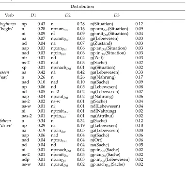
Table 1 presents three verbs from different classes and their 10 most frequent frame types at the three levels of verb definition and their probabilities.D1 forbeginnen‘begin’ defines ‘np’ and ‘n’ as the most probable frame types. After splitting the ‘np’ probability over the different PP types inD2, a number of prominent PPs are left, the time indicat-ing umAcc andnachDat,mitDat referring to the begun event,anDat as date, and inDat as
place indicator. It is obvious that not all PPs are argument PPs, but adjunct PPs also represent a part of the verb behavior.D3 illustrates that typical selectional preferences for beginner roles are Situation ‘situation’, Zustand ‘state’, Zeit ‘time’, Sache ‘thing’. D3 has the potential to indicate verb alternation behavior, for example, ‘na(Situation)’ refers to the same role for the direct object in a transitive frame as “n(Situation)” in an intransitive frame. essen‘eat’ as an object-drop verb shows strong preferences for both intransitive and transitive usage. As desired, the argument roles are dominated by Lebewesen ‘creature’ for ‘n’ and ‘na’ and Nahrung ‘food’ for ‘na’. fahren ‘drive’ chooses typical manner of motion frames (‘n,’ ‘np,’ ‘na’) with the refining PPs being directional (inAcc, zuDat, nachDat) or referring to a means of motion (mitDat, inDat, aufDat).
The selectional preferences show correct alternation behavior: Lebewesen ‘creature’ in the object drop case for ‘n’ and ‘na,’Sache ‘thing’ in the inchoative/causative case for ‘n’ and ‘na’.
In addition to the absolute verb descriptions above, a simple smoothing technique is applied to the feature values. The goal of smoothing is to create more uniform distributions, especially with regard to adjusting zero values, but also for assimilating high and low frequencies and probabilities. The smoothed distributions are particularly interesting for distributions with a large number of features, since they typically contain
Table 1
Example distributions of German verbs.
Distribution
Verb D1 D2 D3
beginnen np 0.43 n 0.28 n(Situation) 0.12
‘begin’ n 0.28 np:umAcc 0.16 np:umAcc(Situation) 0.09 ni 0.09 ni 0.09 np:mitDat(Situation) 0.04 na 0.07 np:mitDat 0.08 ni(Lebewesen) 0.03
nd 0.04 na 0.07 n(Zustand) 0.03
nap 0.03 np:anDat 0.06 np:anDat(Situation) 0.03 nad 0.03 np:inDat 0.06 np:inDat(Situation) 0.03
nir 0.01 nd 0.04 n(Zeit) 0.03
ns-2 0.01 nad 0.03 n(Sache) 0.02
xp 0.01 np:nachDat 0.01 na(Situation) 0.02
essen na 0.42 na 0.42 na(Lebewesen) 0.33
‘eat’ n 0.26 n 0.26 na(Nahrung) 0.17
nad 0.10 nad 0.10 na(Sache) 0.09
np 0.06 nd 0.05 n(Lebewesen) 0.08
nd 0.05 ns-2 0.02 na(Lebewesen) 0.07
nap 0.04 np:aufDat 0.02 n(Nahrung) 0.06
ns-2 0.02 ns-w 0.01 n(Sache) 0.04
ns-w 0.01 ni 0.01 nd(Lebewesen) 0.04
ni 0.01 np:mitDat 0.01 nd(Nahrung) 0.02 nas-2 0.01 np:inDat 0.01 na(Attribut) 0.02
fahren n 0.34 n 0.34 n(Sache) 0.12
‘drive’ np 0.29 na 0.19 n(Lebewesen) 0.10
na 0.19 np:inAcc 0.05 na(Lebewesen) 0.08
nap 0.06 nad 0.04 na(Sache) 0.06
nad 0.04 np:zuDat 0.04 n(Ort) 0.06
nd 0.04 nd 0.04 na(Sache) 0.05
ni 0.01 np:nachDat 0.04 np:inAcc(Sache) 0.02 ns-2 0.01 np:mitDat 0.03 np:zuDat(Sache) 0.02 ndp 0.01 np:inDat 0.03 np:inAcc(Lebewesen) 0.02 ns-w 0.01 np:aufDat 0.02 np:nachDat(Sache) 0.02
persuasive zero values and severe outliers. Chen and Goodman (1998) present a concise overview of smoothing techniques, with specific emphasis on language modeling. We decided to apply the smoothing algorithm referred to asadditive smoothing: The smooth-ing is performed simply by addsmooth-ing 0.5 to all verb features, that is, the joint frequency of each verbvand featurexiis changed by freq(v,xi)=freq(v,xi)+0.5. The total verb
frequency is adapted to the changed feature values, representing the sum of all verb feature values: vfreq=
ifreq(v,xi). Smoothed probability values are based on the
smoothed frequency distributions.
2.3 Clustering Algorithm and Evaluation Techniques
generalizing over the data objects and their features. The clustering of the German verbs is performed by thek-means algorithm, a standard unsupervised clustering technique as proposed by Forgy (1965). Withk-means, initial verb clusters are iteratively reorgan-ized by assigning each verb to its closest cluster and recalculating cluster centroids until no further changes take place. Applying thek-means algorithm assumes (1) that verbs are represented by distributional vectors and (2) that verbs that are closer to each other in a mathematically defined way are also more similar to each other in a linguistic way.k-Means depends on the following parameters: (1) The number of clusters is not known beforehand, so the clustering experiments investigate this parameter. Related to this parameter is the level of semantic concept: The more verb clusters are found, the more specific the semantic concept, and vice versa. (2)k-means is sensitive to the initial clusters, so the initialization is varied according to how much preprocessing we invest: Both random clusters and hierarchically preprocessed clusters are used as initial clusters for k-means. In the case of preprocessed clusters, the hierarchical clustering is performed as bottom-up agglomerative clustering with the following criteria for merging the clusters: single linkage (minimal distance between nearest neighbor verbs), complete linkage (minimal distance between furthest neighbor verbs), average distance between verbs, distance between cluster centroids, and Ward’s method (minimizing the sum of squares when merging clusters). The merging method influences the shape of the clusters; for example, single linkage causes a chaining effect in the shape of the clusters, and complete linkage creates compact clusters. (3) In addition, there are several possibilities for defining the similarity between distributional vectors. But which best fits the idea of verb similarity? Table 2 presents an overview of relevant similarity measures that are applied in the experiments.xandyrefer to the verb object vectors, their subscripts to the verb feature values. The Minkowski metric can be applied to frequencies and probabilities. It is a generalization of the two well-known instances q=1 (Manhattan distance) andq=2 (Euclidean distance). TheKullback–Leibler divergence (KL)is a measure from information theory that determines the inefficiency of assuming a model probability distribution given the true distribution (Cover and Thomas 1991). The KL divergence is not defined in caseyi=0, so the probability distributions need
to be smoothed. Two variants of KL,information radius andskew divergence, perform a default smoothing. Both variants can tolerate zero values in the distribution because they work with a weighted average of the two distributions compared. Lee (2001) has shown that the skew divergence is an effective measure for distributional similarity in NLP. Similarly to Lee’s method, we set the weightwfor the skew divergence to 0.9. The cosinemeasures the similarity of the two object vectorsxandyby calculating the cosine of the angle between the feature vectors. The cosine measure can be applied to frequency and probability values. For a detailed description of hierarchical clustering techniques and an intuitive interpretation of the similarity measures, the reader is referred to, for example, Kaufman and Rousseeuw (1990).
Table 2
Data similarity measures.
Measure Definition
Minkowski metric /Lqnorm Lq(x,y)= q n
i=1|xi−yi|q
Manhattan distance /L1norm L1(x,y)=
n
i=1|xi−yi|
Euclidean distance /L2norm L2(x,y)=ni=1(xi−yi)2
KL divergence / relative entropy D(x||y)=in=1 xi ∗ log xyii
Information radius IRad(x,y)=D(x||x+2y) + D(y||x+2y)
Skew divergence Skew(x,y)=D(x||w∗y + (1−w)∗x)
Cosine cos(x,y)=
n i=1xi∗yi n
i=1x2i ∗ n
i=1y2i
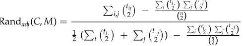
percentage. (2) The adjusted Rand index is a measure of agreement versus disagreement between object pairs in clusterings that provides the most appropriate reference to a null model (Hubert and Arabie 1985); cf. equation (1). The agreement in the two partitions is represented by a contingency tableC×M:tijdenotes the number of verbs
common to classesCi in the clustering partitionCandMj in the manual classification M; the marginalsti.andt.jrefer to the number of objects inCiandMj, respectively; the
expected number of common object pairs attributable to a particular cellCi,Mjin the
contingency table is defined byti.
2
t.j 2
/n2
. The upper bound for Randadjis 1, the lower
bound is mostly 0, with only extreme cases below zero.
Randadj(C,M)=
i,j
tij 2
− i(ti2.)
j( t.j
2) (n
2)
1 2 (
i
ti.
2
+ jt.j 2
) −
i(ti2.)
j( t.j
2) (n
2)
(1)
The above two measures were chosen as a result of comparing various evaluation measures and their properties with respect to the linguistic task (Schulte im Walde 2003a, chapter 4).
3. Preliminary Clustering Experiments
3.1 Baseline and Upper Bound
The experiment baseline refers to 50 random clusterings: The verbs are randomly as-signed to a cluster (with a cluster number between 1 and the number of manual classes), and the resulting clustering is evaluated by the evaluation measures. The baseline value is the average value of the 50 repetitions. The upper bound of the experiments (the “optimum”) refers to the evaluation values on the manual classification; the manual classification is adapted before calculating the upper bound by randomly deleting additional senses (i.e., more than one sense) of a verb, so as to leave only one sense for each verb, sincek-means as a hard clustering algorithm cannot model ambiguity. Table 3 lists the baseline and upper bound values for the clustering experiments.
3.2 Experiment Results
The following tables present the results of the clustering experiments. Tables 4 to 7 each concentrate on one technical parameter of the clustering process; Tables 8 to 10 then focus on performing clustering with a fixed parameter set, in order to vary the linguistically interesting parameters concerning the feature choice for the verbs. All significance tests have been performed withχ2,df =1,α=0.05.
Table 4 illustrates the effect of thedistribution units(frequencies and probabilities) on the clustering result. The experiments use distributions onD1 andD2 with random and preprocessed initialization, and the cosine as similarity measure (since it works for both distribution units). To summarize the results, neither the differences between frequencies and probabilities nor between original and smoothed values are significant. Table 5 illustrates the usage of different similarity measures.As before, the exper-iments are performed for D1 and D2 with random and preprocessed initialization. The similarity measures are applied to the relevant probability distributions (as the distribution unit that can be used for all measures). The tables point out that there is no best-performing similarity measure in the clustering processes. On the larger feature set, the Kullback–Leibler variants information radius and skew divergence tend to outperform all other similarity measures. In fact, the skew divergence is the only measure that shows significant differences for some parameter settings, as compared to all other measures except information radius. In further experiments, we will therefore concentrate on the two Kullback–Leibler variants.
Tables 6 and 7 compare the effects of varying the initialization of the k-means algorithm. The experiments are performed for D1 and D2 with probability distrib-utions, using the similarity measures information radius and skew divergence. For random and hierarchical initialization, we cite both the evaluation scores for the k-means initial cluster analysis (i.e., the output clustering from the random assignment or the preprocessing hierarchical analysis), and for the k-means result. The manual columns in the tables refer to a cluster analysis where the initial clusters provided to
Table 3
k-means experiment baseline and upper bound.
Evaluation Baseline Optimum
PairF 2.08 95.81
Table 4
Comparing distributions onD1 andD2.
Distribution:D1 Distribution:D2 Probability Frequency Probability Frequency Eval Initial Original Smoothed Original Smoothed Original Smoothed Original Smoothed PairF Random 12.67 12.72 14.06 14.14 14.98 15.37 14.82 15.07
H-Ward 11.40 11.70 11.56 11.37 10.57 13.71 11.65 9.98 Randa Random 0.090 0.090 0.102 0.102 0.104 0.113 0.107 0.109
[image:15.486.54.442.235.321.2]H-Ward 0.079 0.081 0.080 0.076 0.065 0.096 0.075 0.056
Table 5
Comparing similarity measures onD1 andD2.
Similarity Measure
D1 D2
Eval Initial Cos L1 Eucl IRad Skew Cos L1 Eucl IRad Skew PairF Random 12.67 13.11 13.85 14.19 14.13 14.98 15.20 16.10 16.15 18.01
H-Ward 11.40 13.65 12.88 13.07 12.64 10.57 15.51 13.11 17.49 19.30 Randa Random 0.090 0.094 0.101 0.101 0.105 0.104 0.109 0.123 0.118 0.142
H-Ward 0.079 0.099 0.093 0.097 0.094 0.065 0.116 0.092 0.142 0.158
Table 6
Comparing clustering initializations onD1.
k-means Initialization Random Eval Distance Manual Best Avg PairF IRad 18.56 2.16→14.19 11.78 Skew 20.00 1.90→14.13 12.17 Randa IRad 0.150 −0.004→0.101 0.078
Skew 0.165 −0.005→0.105 0.083
k-means Initialization Hierarchical
Eval Distance Single Complete Average Centroid Ward PairF IRad 4.80→12.73 9.43→10.16 10.83→11.33 8.77→11.88 12.76→13.07
Skew 4.81→13.04 11.50→11.00 11.68→11.41 8.83→11.45 12.44→12.64 Randa IRad 0.000→0.088 0.055→0.065 0.067→0.072 0.039→0.079 0.094→0.097 Skew 0.000→0.090 0.077→0.072 0.075→0.073 0.041→0.072 0.092→0.094
[image:16.486.48.441.477.665.2]The overall results are better than for single linkage, but only slightly improved by k-means. Hierarchical clusters as based on complete-linkage amalgamation are more compact, and result in a closer fit to the gold standard than the previous methods. The hierarchical initialization is only slightly improved by k-means; in some cases the k-means output is worse than its hierarchical initialization. Ward’s method seems to work best on hierarchical clusters andk-means initialization. The cluster sizes are more balanced and correspond to compact cluster shapes. As for complete linkage, k-means improves the clusterings only slightly; in some cases the k-means output is worse than its hierarchical initialization. A cluster analysis based on Ward’s hierarchical clusters performs best of all the applied methods, especially with an increasing number of features. The similarity of Ward’s clusters (and similarly complete linkage clusters)
Table 7
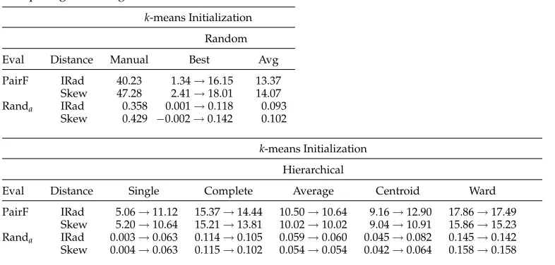
Comparing clustering initializations onD2.
k-means Initialization Random Eval Distance Manual Best Avg PairF IRad 40.23 1.34→16.15 13.37
Skew 47.28 2.41→18.01 14.07 Randa IRad 0.358 0.001→0.118 0.093
Skew 0.429 −0.002→0.142 0.102
k-means Initialization Hierarchical
Eval Distance Single Complete Average Centroid Ward PairF IRad 5.06→11.12 15.37→14.44 10.50→10.64 9.16→12.90 17.86→17.49
andk-means is not by chance, since these methods aim to optimize the same criterion, the sum of distances between the verbs and their respective cluster centroids. Note that for D2, Ward’s method actually significantly outperforms all other initialization methods, complete linkage significantly outperforms all but Ward’s. Between single linkage, average and centroid distance, there are no significant differences. ForD1, there are no significant differences between the initializations.
The low scores in the tables might be surprising to the reader, but they reflect the difficulty of the task. As mentioned before, we deliberately set high demands for the gold standard, especially with reference to the fine-grained, small classes. Compared to related work (cf. Section 5), our results achieve lower scores because the task is more difficult; for example, Merlo and Stevenson (2001) classify 60 verbs into 3 classes, and Siegel and McKeown (2000) classify 56 verbs into 2 classes, as compared to our clustering, which assigns 168 verbs to 43 classes. The following illustrations should provide an intuition about the difficulty of the task:
1. In a set of additional experiments, a random choice of a reduced number of 5/10/15/20 classes from the gold standard is performed. The verbs from the respective gold standard classes are clustered with the optimal parameter set (see Table 8), which results in a pairwise f-scorePairFof 22.19%. The random choice and the cluster analysis are repeated 20 times for each reduced gold standard size of 5/10/15/20 classes, and the averagePairFis calculated: The results are 45.27/35.64/30.30/26.62%, respectively. This shows that the clustering results are much better (with the same kind of data and features and the same algorithm) when applied to a smaller number of verbs and classes.
2. Imagine a gold standard of three classes with four members each, for example,{{a, b, c, d},{e, f, g, h},{i, j, k, l}}. If a cluster analysis of these elements into three clusters resulted in an almost perfect choice of{{a, b, c, d, e},{f, g, h},{i, j, k, l}}where onlyeis assigned to a ”wrong” class, the pairwise precision is 79%, the recall is 83%, andpairFis 81%, so the decrease ofpairFwith only one mistake is almost 20%. If another cluster analysis resulted in a choice with just one more mistake such as{{a, b, c, d, e, i},{f, g, h},{j, k, l}}whereiis also assigned to a ”wrong” class, the result decreases by almost another 20%, to a precision of 57%, a recall of 67%, andpairFof 62%. The results show how much impact a few mistakes may have on the pairwisef-score of the results.
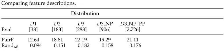
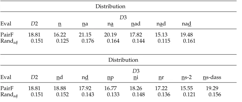
The last series of experiments applies the algorithmic insights from the previous experiments to a linguistic variation of parameters (cf. Schulte im Walde 2003b). The verbs are described by probability distributions on different levels of linguistic infor-mation (frames, prepositional phrases, and selectional preferences). A preprocessing hierarchical cluster analysis is performed by Ward’s method, and k-means is applied to re-organize the clusters. Similarities are measured by the skew divergence. Table 8 presents the first results comparingD1,D2, andD3, either on specified frame slots (‘n,’ ‘na,’ ‘nd,’ ‘nad,’ ‘ns-dass’), on all noun phrase slots (NP), or on all noun phrase and prepositional phrase slots (NP–PP). The number of features in each experiment is given in square brackets. The table demonstrates that a purely syntactic verb description gives rise to a verb clustering clearly above the baseline. Refining the coarse subcategorization frames with prepositional phrases considerably improves the verb clustering results. Adding selectional preferences to the verb description further improves the clustering results, but the improvement is not as persuasive as in the first step, when refining the purely syntactic verb descriptions with prepositional information. The difference between D1 and D2 is significant, but neither the difference between D2 and D3 (in any variation) nor the differences between the variants ofD3 are significant. In the case of adding role information to all NP (and all PP) slots, the problem might be caused by sparse data, but for the linguistically chosen subset of argument slots we assume additional linguistic reasons are directly relevant to the clustering outcome.
[image:18.486.47.433.575.664.2]In order to choose the most informative frame roles forD3, we varied the selectional preference slots by considering only single slots for refinements, or small combinations of argument slots. The variations should provide insight into the contribution of slots and slot combinations to the clustering. The experiments are performed on probability distributions for D3; all other parameters were chosen as above. Table 9 shows that refining only a single slot (the underlined slot in the respective frame type) in addition to the D2 definitions results in little or no improvement. There is no frame-slot type that consistently improves results, but success depends on the parameter instantiation. The results do not match our linguistic intuitions: For example, we would expect the arguments in the two highly frequent intransitive ‘na’ and transitive ‘na’ frames with variable semantic roles to provide valuable information with respect to their selectional preferences, but only those in ‘na’ actually improveD2. However, a subject in a transi-tive construction with a non-finite clause ‘ni’, which is less variable with respect to verbs and roles, does work better than ‘n’. In Table 10, selected slots are combined to define selectional preference information, for example, n/na means that the nominative slot in ‘na’, and both the nominative and accusative slot in ‘na’ are refined by selectional preferences. It is obvious that the clustering effect does not represent a sum of its parts, for example, both the information in ‘na’ and in ‘na’ improve Ward’s clustering based on D2 (cf. Table 9), but it is not the case that ‘na’ improves the clustering, too.
Table 8
Comparing feature descriptions.
Distribution
D1 D2 D3 D3 NP D3 NP–PP
Eval [38] [183] [288] [906] [2,726]
Table 9
Comparing selectional preference slot definitions.
Distribution
D3
Eval D2 n na na nad nad nad
PairF 18.81 16.22 21.15 20.19 17.82 15.13 19.48 Randadj 0.151 0.125 0.176 0.164 0.144 0.115 0.161
Distribution
D3
Eval D2 nd nd np ni nr ns-2 ns-dass
PairF 18.81 18.88 17.92 16.77 18.26 17.22 15.55 19.29 Randadj 0.151 0.152 0.143 0.133 0.148 0.136 0.121 0.156
As in Table 9, there is no combination of selectional preference frame definitions that consistently improves the results. On the contrary, some additional D3 information makes the result significantly worse, for example, ‘nad’. The specific combination of selectional preferences as determined preexperimentally actually achieves the overall best results, better than any other slot combination, and better than refining all NP slots or refining all NP and all PP slots in the frame types (cf. Table 8).
3.3 Experiment Interpretation
[image:19.486.52.448.501.666.2]For illustrative purposes, we present representative parts of the cluster analysis as based on the following parameters: The clustering initialization is obtained from a hierarchical analysis of the German verbs (Ward’s amalgamation method), the number of clusters being the number of manual classes (43); the similarity measure is the skew divergence. The cluster analysis is based on the verb description on D3, with selectional roles for
Table 10
Comparing selectional preference frame definitions.
Distribution
D3
Eval D2 n na n/na nad n/na/nad
PairF 18.81 16.22 17.82 17.00 13.36 16.05 Randadj 0.151 0.125 0.137 0.128 0.088 0.118
Distribution
D3
Eval D2 nd n/na/nd n/na/nad/nd np/ni/nr/ns-2/ns-dass
PairF 18.81 18.48 16.48 20.21 16.73
‘n,’ ‘na,’ ‘nd,’ ‘nad,’ ‘ns-dass.’ We compare the clusters with the respective clusters by D1 andD2.
(a) nieseln regnen schneien –Weather (b) d¨ammern –Weather
(c) beginnen enden –Aspect bestehen existieren –Existence liegen sitzen stehen –Position
laufen –Manner of Motion: Locomotion
(d) kriechen rennen –Manner of Motion: Locomotion eilen –Manner of Motion: Rush
gleiten –Manner of Motion: Flotation starren –Facial Expression
(e) klettern wandern –Manner of Motion: Locomotion fahren fliegen segeln –Manner of Motion: Vehicle fließen –Manner of Motion: Flotation
(f) festlegen –Constitution bilden –Production
erh ¨ohen senken steigern vergr ¨oßern verkleinern –Quantum Change (g) t ¨oten –Elimination
unterrichten –Teaching
(h) geben –Transfer of Possession (Giving): Gift
selectional preferences help to distinguish this cluster: The verbs agree in demanding a thing or situation as subject, and various objects such as attribute, cognitive object, state, structure, or thing as object. Without selectional preferences (onD1 andD2), the change of quantum verbs are not found together with the same degree of purity. There are verbs as in cluster (g) whose properties are correctly stated as similar byD1–D3, so a common cluster is justified, but the verbs only have coarse common meaning components; in this caset¨oten‘kill’ andunterrichten‘teach’ agree in an action of one person or institution towards another.gebenin cluster (h) represents a singleton. Syntactically, this is caused by being the only verb with a strong preference for “xa.” From the meaning point of view, this specific frame represents an idiomatic expression, only possible withgeben.
An overall interpretation of the clustering results gives insight into the relationship between verb properties and clustering outcome. (1) The fact that there are verbs that are clustered semantically on the basis of their corpus-based and knowledge-based empirical properties indicates (a) a relationship between the meaning components of the verbs and their behavior and (b) that the clustering algorithm is able to benefit from the linguistic descriptions and to abstract away from the noise in the distributions. (2) Low-frequency verbs were a problem in the clustering experiments. Their distributions are noisier than those for more frequent verbs, so they typically constitute noisy clusters. (3) As known beforehand, verb ambiguity cannot be modeled by the hard clustering algorithm k-means. Ambiguous verbs were typically assigned either (a) to one of the correct clusters or (b) to a cluster whose verbs have distributions that are similar to the ambiguous distribution, or (c) to a singleton cluster. (4) The interpretation of the clusterings unexpectedly points to meaning components of verbs that have not been discovered by the manual classification. An example verb islaufen, expressing not only aManner of Motionbut also a kind of existence when used in the sense of operation. The discovery effect should be more impressive with an increasing number of verbs, since manual judgement is more difficult, and also with a soft clustering technique, where multiple cluster assignment is enabled. (5) In a similar way, the clustering interpretation exhibits semantically related verb classes, that is, verb classes that are separated in the manual classification, but semantically merged in a common cluster. For example, PerceptionandObservationverbs are related in that all the verbs express an observation, with thePerceptionverbs additionally referring to a physical ability, such as hearing. (6) Related to the preceding issue, the manual verb classes as defined are demonstrated as detailed and subtle. Compared to a more general classification that would appropriately merge several classes, the clustering confirms that we defined a difficult task with subtle classes. We were aware of this fact but preferred a fine-grained classification, since it allows insight into verb and class properties. In this way, verbs that are similar in meaning are often clustered incorrectly with respect to the gold standard.
The improvement underlines the linguistic fact that verbs that are similar in their meaning agree either on a specific prepositional complement (e.g.,glauben/denken anAcc)
or on a more general kind of modification, for example, directional PPs forManner of Motionverbs. (3) Defining selectional preferences for arguments improves the clustering results further, but the improvement is not as persuasive as when refining the purely syntactic verb descriptions with prepositional information. For example, selectional preferences help demarcate theQuantum Changeclass because the respective verbs agree in their structural as well as selectional properties. But in theConsumptionclass,essen and trinken have strong preferences for a food object, whereas konsumieren allows a wider range of object types. In contrast, there are verbs that are very similar in their behavior, especially with respect to a coarse definition of selectional roles, but they do not belong to the same fine-grained semantic class, for example,t¨otenandunterrichten. The effect could be due to (a) noisy or (b) sparse data, but the basic verb descriptions appear reliable with respect to their desired linguistic content, and Table 8 illustrates that even with little added information the effect exists (e.g., refining few arguments by 15 selectional roles results in 253 instead of 178 features, so the magnitude of feature numbers does not change). Why do we encounter an indeterminism concerning the encoding and effect of verb features, especially with respect to selectional preferences? The meaning of verbs comprises both properties that are general for the respective verb classes, and idiosyncratic properties that distinguish the verbs from each other. As long as we define the verbs by those properties that represent the common parts of the verb classes, a clustering can succeed. But by stepwise refining the verb description and including lexical idiosyncrasy, the emphasis on the common properties vanishes. From a theoretical point of view, the distinction between common and idiosyncratic features is obvious, but from a practical point of view there is no perfect choice for the encoding of verb features. The feature choice depends on the specific properties of the desired verb classes, and even if classes are perfectly defined on a common conceptual level, the relevant level of behavioral properties of the verb classes might differ. Still, for a large-scale classification of verbs, we need to specify a combination of linguistic verb features as a basis for the clustering. Which combination do we choose? Both the theoretical assumption of encoding features of verb alternation as verb behavior and the practical realization by encoding syntactic frame types, prepositional phrases, and selectional preferences seem promising. In addition, we aimed at a (rather linguistically than technically based) choice of selectional preferences that represents a useful compromise for the conceptual needs of the verb classes. Therefore, this choice of features best utilizes the meaning–behavior relationship and will be applied in a large-scale clustering experiment (cf. Section 4).
3.4 Optimizing the Number of Clusters
methodology might be successful in capturing a rough verb classification with few verb classes but not a fine-grained classification with many subtle distinctions.
Figure 1 illustrates the clustering results for the series of cluster analyses as performed by k-means with hierarchical clustering initialization (Ward’s method) on probability distributions, with skew divergence as the similarity measure. The feature description refers toD2. The number of clusters is varied from 1 through the number of verbs (168), and the results are evaluated by Randadj. A range of numbers of clusters
is determined as optimal (71) or near-optimal (approx. 58–78). The figure demonstrates that having performed experiments on the parameters for clustering, it is worthwhile exploring additional parameters: The optimal result is 0.188 for 71 clusters as compared to 0.158 for 43 clusters reported previously.
4. Large-Scale Clustering Experiments
So far, all clustering experiments were performed on a small scale, preliminary set of 168 manually chosen German verbs. One goal of this article was to develop a clustering methodology with respect to the automatic acquisition of a large-scale German verb classification. We therefore apply the insights on the theoretical relationship between verb meaning and verb behavior and our findings regarding the clustering parameters to a considerably larger amount of verb data.
[image:23.486.58.363.405.643.2]We extracted all German verbs from our statistical grammar model that appeared with an empirical frequency of between 500 and 10,000 in the training corpus (cf. Section 2.2). This selection resulted in a total of 809 verbs, including 94 verbs from the preliminary set of 168 verbs. We added the missing verbs from the preliminary set, resulting in a total of 883 German verbs. The feature description of the German verbs refers to the probability distribution over the coarse syntactic frame types, with
Figure 1
prepositional phrase information on the 30 chosen PPs and selectional preferences for our empirically most successful combination ‘n,’ ‘na,’ ‘nd,’ ‘nad,’ and ‘ns-dass.’ As in previous clustering experiments, the features are stepwise refined.k-means is provided hierarchical clustering initialization (based on Ward’s method), with the similarity mea-sure being skew divergence. The number of clusters is set to 100, which corresponds to an average of 8.83 verbs per cluster, that is, not too fine-grained clusters but still possible to interpret. The preliminary set of 168 verbs is a subset of the large-scale set in order to provide an “auxiliary” evaluation of the clustering results: Considering only the manually chosen verbs in the clustering result, this partial cluster analysis is evaluated against the gold standard of 43 verb classes. Results were not expected to match the results of our clustering experiments using only the preliminary verb set, but to provide an indication of how different cluster analyses can be compared with each other.
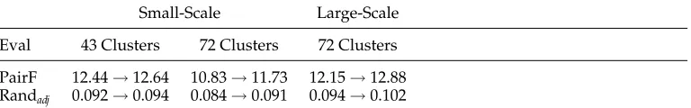
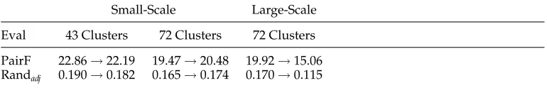
Tables 11 to 13 present the clustering results for the large-scale verb set forD1–D3 in the rightmost columns, citing the evaluation scores of the initial (hierarchical) clusters and the resultingk-means clusters. The subset of the 168 gold standard verbs is scattered over 72 of the 100 resulting clusters. The results are compared to our previous results for the 168 verbs in 43 clusters, and to the case where those 168 verbs are clustered into 72 hierarchical classes. The large-scale clustering results once more confirm the general insights (1) that the stepwise refinement of features improves the clustering and (2) that Ward’s hierarchical clustering is seldom improved by thek-means application. In addition, several of the large-scale cluster analyses were quite comparable with the clustering results using the small-scale set of verbs, especially when compared to 72 clusters.
In the following, we present example clusters from the optimal large-scale cluster analysis (according to the above evaluation): Ward’s hierarchical cluster analysis based on subcategorization frames, PPs, and selectional preferences, without runningk-means on the hierarchical clustering. Some clusters are extremely good with respect to the se-mantic overlap of the verbs, some clusters contain a number of similar verbs mixed with semantically different verbs, and for some clusters it is difficult to recognize common elements of meaning. The verbs that we think are semantically similar are marked in bold face.
(1) abschneiden‘cut off’,anziehen‘dress’,binden‘bind’,entfernen‘remove’, tunen‘tune’,wiegen‘weigh’
[image:24.486.50.434.601.661.2](2) aufhalten‘detain’,aussprechen‘pronounce’,auszahlen‘pay off’,durchsetzen ‘achieve’,entwickeln‘develop’,verantworten‘be responsible’,verdoppeln ‘double’,zur ¨uckhalten‘keep away’,zur ¨uckziehen‘draw back’,¨andern ‘change’
Table 11
Large-scale clustering onD1.
Small-Scale Large-Scale
Eval 43 Clusters 72 Clusters 72 Clusters
Table 12
Large-scale clustering onD2.
Small-Scale Large-Scale
Eval 43 Clusters 72 Clusters 72 Clusters
[image:25.486.53.438.212.274.2]PairF 18.64→18.81 17.56→18.81 18.22→16.96 Randadj 0.148→0.151 0.149→0.161 0.152→0.142
Table 13
Large-scale clustering onD3 with n/na/nd/nad/ns-dass.
Small-Scale Large-Scale
Eval 43 Clusters 72 Clusters 72 Clusters
PairF 22.86→22.19 19.47→20.48 19.92→15.06 Randadj 0.190→0.182 0.165→0.174 0.170→0.115
(3) anh¨oren‘listen’,auswirken‘affect’,einigen‘agree’,lohnen‘be worth’, verhalten‘behave’,wandeln‘promenade’
(4) abholen‘pick up’,ansehen‘watch’,bestellen‘order’,erwerben‘purchase’,
holen‘fetch’,kaufen‘buy’,konsumieren‘consume’,verbrennen‘burn’,
verkaufen‘sell’
(5) anschauen‘watch’,erhoffen‘wish’,vorstellen‘imagine’,w ¨unschen‘wish’, ¨uberlegen‘think about’
(6) danken‘thank’,entkommen‘escape’,gratulieren‘congratulate’
(7) beschleunigen‘speed up’,bilden‘constitute’,darstellen‘illustrate’,decken ‘cover’,erf ¨ullen‘fulfil’,erh ¨ohen‘raise’,erledigen‘fulfil’,finanzieren ‘finance’,f ¨ullen‘fill’,l¨osen‘solve’,rechtfertigen‘justify’,reduzieren
‘reduce’,senken‘lower’,steigern‘increase’,verbessern‘improve’,
vergr ¨oßern‘enlarge’,verkleinern‘make smaller’,verringern‘decrease’,
verschieben‘shift’,versch ¨arfen‘intensify’,verst ¨arken‘intensify’,
ver ¨andern‘change’
(8) ahnen‘guess’,bedauern‘regret’,bef ¨urchten‘fear’,bezweifeln‘doubt’,
merken‘notice’,vermuten‘assume’,weißen‘whiten’,wissen‘know’ (9) anbieten‘offer’,bieten‘offer’,erlauben‘allow’,erleichtern‘facilitate’,
erm ¨oglichen‘make possible’,er ¨offnen‘open’,untersagen‘forbid’, veranstalten‘arrange’,verbieten‘forbid’
(10) argumentieren‘argue’,berichten‘report’,folgern‘conclude’,hinzuf ¨ugen
‘add’,jammern‘moan’,klagen‘complain’,schimpfen‘rail’,urteilen‘judge’ (11) basieren‘be based on’,beruhen‘be based on’,resultieren‘result from’,
stammen‘stem from’
(12) befragen‘interrogate’,entlassen‘release’,ermorden‘assassinate’,erschießen
(13) beziffern‘amount to’,sch ¨atzen‘estimate’,veranschlagen‘estimate’ (14) entschuldigen‘apologize’,freuen‘be glad’,wundern‘be surprised’,
¨argern‘be annoyed’
(15) nachdenken‘think about’,profitieren‘profit’,reden‘talk’,spekulieren
‘speculate’,sprechen‘talk’,tr ¨aumen‘dream’,verf ¨ugen‘decree’,
verhandeln‘negotiate’
(16) mangeln‘lack’,nieseln‘drizzle’,regnen‘rain’,schneien‘snow’
Clusters (1) to (3) are examples where the verbs do not share elements of meaning. In the overall cluster analysis, such semantically incoherent clusters tend to be rather large, that is, with more than 15–20 verb members. Clusters (4) to (7) are examples of clusters where some of the verbs show overlap in meaning, but also contain con-siderable noise. Cluster (4) mainly contains verbs of buying and selling, cluster (5) contains verbs of wishing, cluster (6) contains verbs of expressing approval, and cluster (7) contains verbs of quantum change. Clusters (8) to (16) are examples of clusters where most or all verbs show a strong similarity in their semantic concept. Cluster (8) contains verbs expressing a propositional attitude; the underlined verbs, in addition, indicate an emotion. The only unmarked verbweißencan be explained, since some of its inflected forms are ambiguous with respect to their base verb: either weißen or wissen, a verb that belongs to the Aspectverb class. The verbs in cluster (9) describe a scene where somebody or some situation makes something possible (in the positive or negative sense); the only exception verb isveranstalten. The verbs in cluster (10) are connected more loosely, all referring to a verbal discussion, with the underlined verbs denoting a negative, complaining way of utterance. In cluster (11) all verbs refer to a basis, in cluster (12) the verbs describe the process from arresting to releasing a suspect, and cluster (13) contains verbs of estimating an amount of money. In cluster (14), all verbs except for entschuldigenrefer to an emotional state (with some origin for the emotion). The verbs in cluster (15) except forprofitierenall indicate thought (with or without talking) about a certain matter. Finally in cluster (16), we can recognize the same weather verb cluster as in the previously discussed small-scale cluster analyses.
We experimented with two variations in the clustering setup: (1) For the selection of the verb data, we considered a random choice of German verbs in approximately the same magnitude of number of verbs (900 verbs plus the preliminary verb set), but without any restriction on the verb frequency. The clustering results are—both on the basis of the evaluation and on the basis of a manual inspection of the resulting clusters—much worse than in the preceding cluster analysis, since the large number of low-frequency verbs destroys the clustering. (2) The number of target clusters was set to 300 instead of 100, that is, the average number of verbs per cluster was 2.94 instead of 8.83. The resulting clusters are numerically slightly worse than in the preceding cluster analysis, but easier for inspection and therefore a preferred basis for a large-scale resource. Several of the large, semantically incoherent clusters are split into smaller and more coherent clusters, and the formerly coherent clusters often preserved their constitution. To present one example, the following cluster from the 100-cluster analysis