http://wrap.warwick.ac.uk/
Original citation:
Chaisemartin, Clément de and D'Haultfoeuille, Xavier (2015) Supplement to fuzzy differences-in-differences. Working Paper. Coventry: University of Warwick. Department of Economics. Warwick economics research papers series (WERPS) (1066).
(Unpublished)
Permanent WRAP url:
http://wrap.warwick.ac.uk/73107
Copyright and reuse:
The Warwick Research Archive Portal (WRAP) makes this work of researchers of the University of Warwick available open access under the following conditions. Copyright © and all moral rights to the version of the paper presented here belong to the individual author(s) and/or other copyright owners. To the extent reasonable and practicable the material made available in WRAP has been checked for eligibility before being made available.
Copies of full items can be used for personal research or study, educational, or not-for-profit purposes without prior permission or charge. Provided that the authors, title and full bibliographic details are credited, a hyperlink and/or URL is given for the original metadata page and the content is not changed in any way.
A note on versions:
The version presented here is a working paper or pre-print that may be later published elsewhere. If a published version is known of, the above WRAP url will contain details on finding it.
Warwick Economics Research Paper Series
Supplement to Fuzzy
Differences-in-Differences
Clement de Chaisemartin and Xavier D'Haultfoeuille
October, 2015
Supplement to Fuzzy Dierences-in-Dierences
Clément de Chaisemartin
∗Xavier D'Haultf÷uille
†October 6, 2015
Abstract
This paper gathers the supplementary material to de Chaisemartin & D'Haultf÷uille (2015). First, we show that two commonly used IV and OLS regressions with time and group xed eects estimate weighted averages of Wald-DIDs. It then follows from Theorem 3.1 in de Chaisemartin & D'Haultf÷uille (2015) that these regressions estimate weighted sums of LATEs, with potentially many negative weights as we illustrate through two applications. We review all papers published in the American Economic Review between 2010 and 2012 and nd that 10.1% of these papers estimate one or the other regression. Second, we consider estimators of the bounds on average and quantile treatment eects derived in Theorems 3.2 and 3.3 in de Chaisemartin & D'Haultf÷uille (2015) and we study their asymptotic behavior. Third, we revisit Gentzkow et al. (2011) and Field (2007) using our estimators. Finally, we present all the remaining proofs not included in the main paper.
1 Fuzzy DID regressions, and their pervasiveness in economics
1.1 Fuzzy DID regressions...
Researchers using fuzzy DID designs usually do not estimate simple regressions with two groups and two periods, but more complex specications with multiple groups and periods. Practices are not unied so details of their specications can vary. In this section, we study two regres-sion specications which have often been used. We show that in both cases, the coecient of treatment is equal to a weighted sum of Wald-DIDs. Following the result of the rst point of Theorem 3.1, it then easy to show that this weighted sum can be rewritten as a weighted sum of the LATEs of switchers in the dierent groups, with potentially many negative weights, as we illustrate through two examples. Therefore, these coecients could lie far from the LATE of switchers in any group.
∗Warwick University, [email protected]
First, we study the coecient of a treatment variableDin a 2SLS regression ofY on a constant,
group dummies(1{G=g})1≤g≤g, time dummies (1{T =t})1≤t≤t, andD, with a rst stage fully
saturated in(T, G). As the rst stage is fully saturated, the second stage is a regression of Y on
a constant, group dummies (1{G = g})1≤g≤g, time dummies (1{T = t})1≤t≤t, and E(D|T, G).
This 2SLS regression is therefore algebraically equivalent to an OLS regression at the group ×
period level ofY on time and group dummies and a measure of treatment intensity in each group × period cell. As shown in the next subsection, such OLS regressions are pervasive in applied
work.
Assume that for every 1 ≤ t ≤ t the mean of treatment does not follow a parallel evolution in
any pair of groups betweent−1and t.1 For every(g, g0, t)∈ {0, ..., g}2× {1, ..., t}, let
DIDD(g, g0, t) = E(Dgt)−E(Dgt−1)−(E(Dg0t)−E(Dg0t−1)),
WDID(g, g0, t) =
E(Ygt)−E(Ygt−1)−(E(Yg0t)−E(Yg0t−1))
E(Dgt)−E(Dgt−1)−(E(Dg0t)−E(Dg0t−1))
.
For(g, t)∈ {1, ..., g} × {1, ..., t}, let
wagt=
DIDD(g, g−1, t)P(G≥g)P(T ≥t) (E(D|G≥g, T≥t)−E(D|G≥g)−E(D|T ≥t) +E(D))
Pt t=1
Pg
g=1DIDD(g, g−1, t)P(G≥g)P(T ≥t) (E(D|G≥g, T≥t)−E(D|G≥g)−E(D|T ≥t) +E(D))
.
For(g, t)∈ {0, ..., g} × {1, ..., t}, let
wbgt =
[E(Dgt)−E(Dgt−1)]P(G=g)P(T ≥t)(E(D|G=g, T≥t)−E(D|G=g)−E(D|T ≥t) +E(D))
Pt t=1
Pg
g=0[E(Dgt)−E(Dgt−1)]P(G=g)P(T ≥t)(E(D|G=g, T≥t)−E(D|G=g)−E(D|T≥t) +E(D))
.
Theorem S1 Letβ denote the coecient of Din a 2SLS regression ofY on a constant, (1{G= g})1≤g≤g, (1{T =t})1≤t≤t, and D, with a rst stage fully saturated in (T, G).
1. If T ⊥⊥G,
β =
t
X
t=1
g
X
g=1
WDID(g, g−1, t)wgta.
2. Morever, if D is binary and Model (1) and Assumptions 1-4 are satised,
β = t
X
t=1
g
X
g=0
∆gtwbgt,
where ∆gt is the LATE of units in group g switching treatment between t−1 and t.
1If for somet, there are groups which experience a parallel evolution of their mean treatment betweent−1and
t, the formula in the rst point of Theorem 1 remains valid after grouping together these groups. The formula
The rst statement of the theorem shows that if T ⊥⊥G, β is a weighted average of Wald-DIDs
between t−1and t and across pairs of groups, for all consecutive dates t−1 and t. With only
two dates, one can order groups according to their increase in treatment between the two dates, thus ensuring that all the weights wgta are positive. With more than two dates, some of the
weightswagt might be negative.
Then, it follows from Theorem 3.1 that whenDis binary and under appropriate common trends
assumptions, each of these Wald-DIDs is equal to a weighted dierence of the LATE of switchers of both groups. Rearranging this sum of weighted dierences yields the second result. A similar result with the same weights holds if treatment is not binary but ordered and with a nite support. A dierence though is that in such instances, β is not equal to a weighted sum of
LATEs but to a weighted sum of the ACRs parameters we introduced in Section 4.3. Some of the weights wb
gt might be negative. With two periods, that will be the case for instance if the
distribution of the changes in treatment between period 0 and 1 across groups is not symmetric around0.
Many papers estimate the regression studied in Theorem 1 with aggregate data at the group
× period level. Results of Theorem 1 still apply to these regressions. We now review three
cases of such group-level regressions which frequently arise in practice. First, when the group level variables are constructed from micro-level variables (e.g.: average wage in county c and
year t) and the OLS regression is weighted by the population in each group × period, the rst
and second statements of Theorem 1 apply as is. Second, when the group level variables are constructed from micro-level variables but the regressions are not weighted, the rst and second statements of Theorem 1 also apply as is, except that now P(G = g) = 1
g for every group.
Note that with unweighted regressions, Gis automatically independent ofT unless some groups
appear or disappear, which is unlikely to be the case when groups are counties, states, or regions. Third, there are instances where all units in each group × period share the same value of the
treatment. This is for instance the case in Gentzkow et al. (2011). When that is the case, the second statement of Theorem 1 actually gets simpler. In such settings, when treatment changes in one group, all units switch treatment. Therefore,∆gt is equal to the average eect of changing
the treatment from its value in period t−1 to its value in period t across all units, normalized
by the change in treatment from periodt−1to t.
We use Theorem 1 to revisit an empirical application. Enikolopov et al. (2011) study the eect of having access to an independent TV channel on the share of people voting for opposition parties in Russia. They regress the share of votes for opposition parties in the 1995 and 1999 elections in regionron region dummies, an indicator for the 1999 election, and on the share of people having
access to the independent TV channel in region r at the time of the election. Figure 1 below
presents the weights wd
g1999 for the 1938 regions in their sample. Regions are ordered according
between the two elections, from the lowest to the largest increase. 1020 weights are negative, and the negative weights sum up to -2.26 (against 3.26 for positive weights: negative weights therefore account for 41% of the sum of the absolute value of weights). If the eect of gaining access to an independent TV channel is heterogeneous across regions where few / many voters gained access to it between 1995 and 1999, the regression coecients in Enikolopov et al. (2011) could lie far from the LATE in any region.
-.005
0
.005
.01
.015
.02
Weight
0 500 1000 1500 2000
[image:6.612.164.440.188.385.2]Counties ordered by their increase in treatment
Figure S 1: wb
gt in Enikolopov et al. (2011).
Second, we study the coecient of a treatment variableDin a 2SLS regression ofY on a constant,
group dummies (1{G=g})1≤g≤g, time dummies (1{T =t})1≤t≤t, and D, where the instrument
for D is equal to f(G)1{T ≥ t0} for some t0 ≥ 1. This specication corresponds exactly to
the one estimated in the rst column and third line of Table 7 in Duo (2001): there f(G) is
the number of schools constructed during the INPRES program in one's district of birth, and
1{T ≥t0}is a dummy for being born late enough to enter school after the program completion.
Let T∗∗ = 1{T ≥ t0}. For any random variable R and for any (g, t) ∈ {0, ..., g} × {0,1}, let
R∗∗gt ∼ R|G = g, T∗∗ = t. Assume that there are no groups where treatment follows a parallel
evolution before and aftert0,2 and let groups be ordered according to their increase of treatment
before and after t0:
E(D∗∗01)−E(D00∗∗)< E(D∗∗11)−E(D10∗∗)< ... < E(Dg∗∗1)−E(Dg∗∗0).
2If there are groups which experience a parallel evolution of their mean treatment, the formula in the rst
For any(g, g0)∈ {0, ..., g}2, let
DIDR∗∗(g, g0) = E(R∗∗g1)−E(R∗∗g0)−(E(R∗∗g01)−E(R∗∗g00)),
WDID∗∗ (g, g0) = DID
∗∗
Y (g, g0) DID∗∗D(g, g0).
Let also
wcg = DID
∗∗
D(g, g−1)P(G≥g)(E(f(G)|G≥g)−E(f(G)))
Pg
g0=1DID∗∗D(g0, g0 −1)P(G≥g0)(E(f(G)|G≥g0)−E(f(G)))
for 1≤g ≤g,
wgd =
E(D∗∗g1)−E(Dg∗∗0)P(G=g)(f(g)−E(f(G)))
Pg
g=0
E(D∗∗
g1)−E(D∗∗g0)
P(G=g)(f(g)−E(f(G))) for 0≤g ≤g.
Theorem S2 Letβ denote the coecient of Din a 2SLS regression ofY on a constant, (1{G= g})1≤g≤g, (1{T =t})1≤t≤t, andD, where the instrument forDwrites asf(G)1{T ≥t0}for some
1≤t0 ≤t.
1. If T ⊥⊥G,
β =
g
X
g=1
WDID∗∗ (g, g−1)wcg.
2. Morever, if D is binary and Model (1) and Assumptions 1-4 are satised with T∗∗ instead
of T,
β = g
X
g=0
∆gwdg,
where ∆g is the LATE of the switchers of group g.
The rst statement of the theorem shows that if T ⊥⊥ G, β is a weighted average of
Wald-DIDs before and aftert0 and across groups with consecutive evolutions of their mean treatment.
Then, it follows from Theorem 3.1 that whenDis binary and under appropriate common trends
assumptions, each of these Wald-DIDs is equal to a weighted dierence of the LATE of switchers of both groups. Rearranging this sum of weighted dierences yields the second result. Here as well, a similar result with the same weights holds if treatment is not binary but ordered and with a nite support. Note that the weights wgd are all positive if and only if all groups where
treatment increases (resp. decreases) have a value off(G) greater (resp. lower) than the mean
of f(G) in the population.
We illustrate this result by estimating the weights wdg for the 284 districts in Duo (2001).
the two cohorts, from the lowest to the largest increase. 132 weights out of 284 are negative, and the negative weights sum up to -3.28 (against 4.28 for positive weights). If switchers' ACRs are heterogeneous across districts with positive and negative weights, the regression coecient in Duo (2001) could lie far from the ACR of switchers in any district.
-.4
-.2
0
.2
.4
Weight
0 100 200 300
[image:8.612.164.441.154.352.2]Districts ordered by their increase in years of schooling
Figure S 2: wd
g in Duo (2001).
1.2 ... and their pervasiveness in economics.
Table S 1: Fuzzy DID papers published in the AER between 2010 and 2012
2010 2011 2012 Total
# papers using the fuzzy DID method 5 15 14 34
% of published papers 5.2% 13.0% 11.2% 10.1%
% of empirical papers, excluding lab experiments 12.8% 24.6% 19.2% 19.7%
We now review each of the 34 papers published by the AER between 2010 and 2012 and which we included in our fuzzy DID count, and carefully justify why their methodology qualies as a fuzzy DID. For each paper, we use the following presentation:
Title of the paper. Where the fuzzy DID method is used in the paper. Why the method used in the paper qualies as a fuzzy DID.
1. Patient Cost-Sharing and Hospitalization Osets in the Elderly. Elasticities of care use to co-payment estimated after Tables 2 and 3.
The elasticity discussed after Table 2 is estimated as the ratio of the eect of the Medicare reform on utilization, divided by the eect of the Medicare reform on co-payment. Both eects are estimated through standard sharp DID specications in Table 2. Therefore, the elasticity estimate is a Wald-DID. Note that even though elasticities do not appear in regression tables, estimating them is one of the main goals of the paper: elasticity estimates are referred to in the abstract.
2. The Eect of Medicare Part D on Pharmaceutical Prices and Utilization. Tables 2 and 3.
In regression equation (1), the dependent variable is the change in the price of drug j between 2003 and 2006, and the explanatory variable is the Medicare market share for drug j in 2003. This regression is equivalent to that studied in Theorem S1, with two periods (2003 and 2006), drug dummies, and a treatment equal to 0 in 2003 and to the Medicare market share of drug j in 2003 in 2006.
3. The Gender Wage Gap and Domestic Violence. Table 2.
In regression equation (2), the dependent variable is the log of female assaults among females of race r in county c in year t, and the explanatory variables are race, year, county, race × year, race × county, and county × year dummies, as well as the gender wage gap
4. Inherited Trust and Growth. Figure 4 and Table 6.
Figure 4 presents a regression of changes in income per capita from 1935 to 2000 on changes in inherited trust over the same period and a constant. This regression is equivalent to that in Theorem S1 with 2 periods, country dummies, and inherited trust as the treatment variable.
5. Inheritance Law and Investment in Family Firms. Table 7.
In the regressions presented in Table 7, the dependent variable is the capital expenditure of rm j in year t, and the explanatory variables are rm dummies, a dummy for whether year t is a succession period for rm j, and the interaction of this dummy with the level of investor protection in the country where rm j is located. This specication is similar to that studied in Theorem S1 with two periods (succession and no succession).
6. Trade Liberalization, Exports, and Technology Upgrading: Evidence on the Impact of MERCOSUR on Argentinian Firms. Tables 3 to 12.
In regression equation (11), the dependent variable is the change in exporting status of rm i in sector j between 1992 and 1996, and the explanatory variable is the change in trade taris in Brasil for products in sector j over the same period. This regression is equivalent to that studied in Theorem S1.
7. Using Loopholes to Reveal the Marginal Cost of Regulation: The Case of Fuel-Economy Standards. Table 5 column 2.
In the regression in Table 5 column (2), the dependent variable is a dummy for whether a car sold is a exible fuel vehicle, and the explanatory variables are state and month dummies, and the percent ethanol availability in each month × state. This regression is
the same as that considered in Theorem S1.
8. What Do Trade Negotiators Negotiate About? Empirical Evidence from the World Trade Organization. Table 3, OLS columns.
In regression equations (15a) and (15b), the dependent variable is the ad valorem tari level bound by country c on product g, while the explanatory variables are country and product xed eects, and two treatment variables which vary at the country × product
level. These regressions are therefore the same as that considered in Theorem S1, except that they have two treatment variables.
9. Group Size and Incentives to Contribute: A Natural Experiment at Chinese Wikipedia. Tables 3 and 4, columns 4-6.
dummy and a measure of social participation by individual i. This regression is the same as that considered in Theorem S1 (treatment is equal to 0 before the block, and to social participation after it).
10. Panic on the Streets of London: Police, Crime, and the July 2005 Terror Attacks. Table 2, Panel C, Columns 3-4.
In regression equation (7), the dependent variable is change in crime rates between week t and the same week one year ago in borough b, and the explanatory variables are a dummy for whether week t is around the terrorist attacks in London, and the number of police forces in borough b in week t. The interaction of the time dummy and of whether borough b belongs to Theseus operation is used as the excluded instrument for police forces. This regression is equivalent to that studied in Theorem S2 (borough xed eects disappear because of the rst dierencing with respect to the previous year, something the authors do to control for seasonality).
11. The Impact of Regulations on the Supply and Quality of Care in Child Care Markets. Table 7, Columns 4 and 5.
In Regression Equation (1), the dependent variable is the outcome for market m in state s in year t, and the explanatory variables are state and year xed eects and a measure of regulations in state s in year t. This regression is the same as that considered in Theorem S1.
12. House Prices, Home Equity-Based Borrowing, and the US Household Leverage Crisis. Tables 2 and 3.
Regression equations (1) and (2) are respectively equivalent to the second and rst stages of the 2SLS regression studied in Theorem S2. Here, everything is in rst dierences between 2006 and 2002. In Theorem S2 we consider the regression in levels but with xed eects so the two specications are equivalent. In levels, the instrument would be the elasticity interacted with the year 2006.
13. State Misallocation and Housing Prices: Theory and Evidence from China. Table 5, Panel A.
outcome before and after the reform and across the two groups of households, divided by the dierence between the value of mismatch in these two groups.
14. The Fundamental Law of Road Congestion: Evidence from US Cities. Table 5. In regression equation (4), the dependent variable is the change in vehicle kilometers traveled in MSA s between periods t and t-1, and the explanatory variable is the change in kilometers of roads in MSA s between periods t and t-1. This regression is almost equivalent to that considered in Theorem S1, except that it does not have time specic constants. The two regressions are equivalent if the eect of time on the outcome is linear. If that is the case, the rst dierences of the time eects in the equation in levelsδt−δt−1
are equal to each other, so estimating the rst-dierence regression with just one constant or with time specic constants will yield the same result.
15. The Consequences of Radical Reform: The French Revolution. Table 3.
In Equation (1), the dependent variable is urbanization in polity j at time t, while the explanatory variables are time and polity dummies, and the number of years of French presence in polity j interacted with the time eects. This regression is equivalent to that studied in Theorem S1.
16. School Desegregation, School Choice, and Changes in Residential Location Patterns by Race.
Table 6. In the regression presented in, say, the rst column of Table 6, the dependent variable is enrolment in schools of MSA j in year t, while the explanatory variables are time and MSA eects and the value of the dissimilarity index of schools in MSA j in year t. The excluded instrument for the dissimilarity index is a dummy for whether in period t, the MSA was desegregated. This regression is the same as that studied in Theorem S2.
17. The Eects of Rural Electrication on Employment: New Evidence from South Africa. Tables 4 and 5 columns 5-8, Table 8 columns 3-4, Table 9 column 2, and Table 10 columns 2, 4, and 6.
Regression equations (3) and (4) are respectively equivalent to the second and rst stages of the 2SLS regression studied in Theorem S2. Here, everything is in rst dierences between the rst and the second wave of the panel. In Theorem S2 we consider the regression in levels but with xed eects so the two specications are equivalent. In Theorem S2, the instrument would be the land gradient Zj interacted with a dummy for the second wave
of the panel.
18. Media and Political Persuation: Evidence from Russia. Table 3.
NTV audience in subregion s in period t. This regression is the same as that studied in Theorem S1.
19. Dynamic Ineciencies in an Employment-Based Health Insurance System: Theory and Evidence. Tables 2, 3, 5, and 6, Column 3.
In regression equation (7), the dependent variable is the health expenditures of individual j working in industry i in period t and region r, and the explanatory variables are individual eects, region specic time eects, and the job tenure of individual j. The death rate of establishments in industry i in period t and region r is used as an instrument for the job tenure of individual j. Within each region, the regression has time eects and individual eects, and an instrument varying only across industry× periods cells. Even though this
instrument does not have the exact same form as that in the regression studied in Theorem S2, these two regressions are close.
20. The Eect of Newspaper Entry and Exit on Electoral Politics. Tables 2 and 3. In regression equation (1), the dependent variable is, say, voter turnout in county c in election year t, and the explanatory variables are county xed eects, state-year eects, and the number of newspapers in county c in year t. Within each state, this regression is the same as that studied in Theorem S1 (within each state, state-year eects become year eects).
21. Americans Do IT Better: US Multinationals and the Productivity Miracle. Table 2, Columns 6-8.
In the regression in, say, column 6 of Table 2, the dependent variable is the log of output per worker in rm i in period t, while the explanatory variables are rms and time xed eects, and the log of the amount of IT capital per employee (ln(C/L)) as well as the
interaction ofln(C/L)and a dummy for whether the rm is owned by a US multinational.
The coecient of ln(C/L) is equal to the same weighted average of Wald-DIDs as the
coecient considered in Theorem S1, within the sample of rms which are not owned by a US multinational. The coecient of the interaction is equal to the dierence between this weighted average in the sample of rms owned by a US multinational, and in the sample of those not owned by a US multinational.
22. Standard Setting Committees: Consensus Governance for Shared Technology Platforms. Table 4, columns 1-3.
conict instead of committee xed eects. If the measure of distributional conict can take only two values, it is easy to show that the coecient of interest τ is equal to the DID of
the outcome across the standards and non-standards track and the low and high value of distributional conict, divided by the dierence between the value of distributional conict in these two groups.
23. Compulsory Licensing: Evidence from the Trading with the Enemy Act. Table 2, columns 3-8.
In the regression equation in the beginning of Section III, the dependent variable is the number of patents by US inventors in patent class c at period t, and the explanatory variables are patent class and time xed eects, and the interaction of period t being after the trading with the enemy act and a measure of treatment intensity. Therefore, this regression is the same as that in Theorem S1 (treatment is equal to 0 before the act).
24. The Internet and Local Wages: A Puzzle. Tables 2 and 4.
In regression equation (1), the dependent variable is the dierence between log wages in 2000 and 1995 in county i, and the explanatory variable is the extent of advanced Internet investment by businesses in county i in 2000. This regression is equivalent to that in Theorem S1. Table 4 presents regressions where advanced internet investment is instrumented by a county level variable. These regressions are equivalent to that in Theorem S2.
25. Estimating the Peace Dividend: The Impact of Violence on House Prices in Northern Ireland. Table 1, columns 3 and 5-7.
In regression equation (1), the dependent variable is the price of houses in region r at time t, while the explanatory variables include region and time xed eects, and the numbers of people killed because of the civil war in region r at time t-1. This regression is the same as that studied in Theorem S1.
26. Paying a Premium on Your Premium? Consolidation in the US Health Insur-ance Industry. Tables 2 and 5.
In regression equation (1), the dependent variable is the change of the log premium for employer e in market m in year t, and explanatory variables are time and market eects, and the change in various treatment variables (change in the fraction of self-insured em-ployees...). This regression is the same as that studied in Theorem S1, except that it has several treatment variables. In regression equation (3), the treatment variables are instrumented by a dummy for periodtbeing after the merger of two insurers and a market
level-variable. This regression is similar to that studied in Theorem S2.
Ad-justments to Environmental Catastrophe. Table 2. In regression equation (1), the dependent variable is, say, the change in log land value in county c between period t and 1930, and the explanatory variables are state× year eects, the share of county c in high
erosion, and the share of county c in medium erosion. Within each state, this regression is equivalent to that in Theorem S1, except that it has two treatment variables.
28. A Rational Expectations Approach to Hedonic Price Regressions with Time-Varying Unobserved Product Attributes: The Price of Pollution. Table 5. In, say, the rst regression equation in the bottom of page 1915, the dependent variable is the change in the price of house j between sales 2 and 3, and the explanatory variables are the change in various pollutants in the area around house j between sales 2 and 3. This regression is equivalent to that in Theorem S1, except that it has several treatment variables.
29. The Impact of Family Income on Child Achievement: Evidence from the Earned Income Tax Credit. Table 3.
In the reduced form of regression equation (4), the dependent variable is the change in test scores for child i between years a and a-1, while the explanatory variable is the change in the expected EITC income of her family based on her family income in year a-1. This regression is equivalent to that considered in Theorem S1, except that it does not have years specic intercepts. The rst stage is the same regression but with the change in the income of the family of student i between years a and a-1. Overall, the 2SLS coecient arising from regression equation (4) is a ratio of 2 weighted averages of Wald-DIDs.
30. Katrina's Children: Evidence on the Structure of Peer Eects from Hurricane Evacuees. Tables 3-6.
In regression equation (1), the dependent variable is the test score of student i in school j in grade g in year t, and the explanatory variables are grade, school, year, and grade ×
year eects, and the fraction of Katrina students received by school j in grade g and year t. Within each grade, this regression is the same as that considered in Theorem S1 (within each grade, grade ×year eects become simple year eects).
31. The Collateral Channel: How Real Estate Shocks Aect Corporate Investment. Table 5.
32. The Spending and Debt Response to Minimum Wage Hikes. Tables 1, 2, and 5. In regression equation (1), the outcome variable is, say, income of household i at period t, and the explanatory variables include household and time dummies, and the minimum wage in the state where household i lives in period t. This regression is the same as that considered in Theorem S1.
33. Exports, Export Destinations, and Skills. Table 5.
In regression equation (7), the dependent variable is a measure of skills in the labor force employed by company i in industry j at period t, and the explanatory variables are rm and industry × time dummies, the ratio of exports to sales in rm i at period t, and
the share of rm exports to high income destinations over total exports. To instrument this variable, the authors use a dummy for the years 1999 or 2000 (a large devaluatation happened in Brazil in 1999) interacted with the share of exports of rm i to Brazil in 1998. This specication is very similar to that studied in Theorem S2.
34. Political Aid Cycles. Table 3, columns 4 and 5, and Tables 4 and 5.
In regression equation (2), the dependent variable is the amount of donations received by receiver r from donor d in year t, and the explanatory variables are donor × receiver
dummies, a dummy for whether there is an election in country r in year t, a measure of alignment between the ruling political parties in countries r and d, and the interaction of the election dummy and the measure of alignment. This specication is very close to that studied in Theorem S1, with units of observation being pairs of donors and receivers.
2 Inference in the partially identied case
In this section, we show how to draw inference on the bounds given in the second statements of Theorems 3.2 and 3.3 in de Chaisemartin & D'Haultf÷uille (2015). We adopt the same notations hereafter. In order for the bounds to be nite, we assume that S(Y) = [y, y] with −∞< y < y <+∞. We also suppose for simplicity that y and y are known by the researcher.3
If not, they can respectively be estimated by mini=1...nYi and maxi=1...nYi, and Theorem S3
below remains valid under regularity conditions onFYd01 at these boundaries.
First, let us consider the Wald-TC bounds. Letbλ0d=
b
P(D01=d)
b
P(D00=d),
b
λ1d=
b
P(D11=d)
b
P(D10=d), and
b
Fd01(y) =M0
h
1−bλ0d(1−FbYd01(y))
i
−M0(1−λb0d)1{y < y},
b
Fd01(y) =m1
h
b
λ0dFbYd01(y) i
+ (1−m1(bλ0d))1{y≥y}.
3In particular, we estimate F−1
Ydgt(0) and F −1
Ydgt(1) by y and y respectively. The denition of Fb −1
Ydgt(τ) for
Then dene
b
δd=
Z
ydFbd01(y)− 1
nd00
X
i∈Id00
Yi, bδd=
Z
ydFbd01(y)−
1 nd00
X
i∈Id00
Yi.
Finally, we estimate the bounds by
c
WT C =
1
n11
P
i∈I11Yi−
1
n10
P
i∈I10
h
Yi+bδDi
i
1
n11
P
i∈I11Di−
1
n10
P
i∈I10Di
, WcT C =
1
n11
P
i∈I11Yi−
1
n10
P
i∈I10
h
Yi+bδD
i
i
1
n11
P
i∈I11Di−
1
n10
P
i∈I10Di
.
Now let us turn to the Wald-CIC bounds. For d∈ {0,1}, let
b
Td=M01
b
λ0dFbYd01−Hb
−1
d (bλ1dFbYd11) b
λ0d−1
!
,Tbd=M01 b
λ0dFbYd01−Hb
−1
d (bλ1dFbYd11+ (1−bλ1d)) b
λ0d−1
!
,
b
Gd(T) =bλ0dFbYd01+ (1−bλ0d)T,Cbd(T) = b
λ1dFbYd11 −Hbd◦Gbd(T) b
λ1d−1
.
We then estimate the bounds on FY11(d)|S1 by
b
FCIC,d(y) = sup y0≤y
b
Cd
b
Td(y0), Fb
CIC,d(y) = inf y0≥yCbd
b
Td
(y0).
Therefore, to estimate bounds for the LATE and LQTE, we use
c
WCIC =
Z
ydFb
CIC,1(y)−
Z
ydFbCIC,0(y), cWCIC = Z
ydFbCIC,1(y)− Z
ydFb
CIC,0(y),
b
τq=Fb −1
CIC,1(q)−Fb −1
CIC,0(q), bτq =Fb −1
CIC,1(q)−Fb
−1
CIC,0(q).
Hereafter, we dene q =FCIC,0(y), q =FCIC,0(y), q1 = [λ11FY111 ◦F
−1
Y101(
1
λ01)−1]/[λ11−1]and
q2 = [λ11FY111◦F
−1
Y101(1−1/λ01)]/[λ11−1]. Our results rely on the following assumptions.
Assumption S1 (Technical conditions for inference with TC bounds)
1. S(Y) = [y, y] with −∞< y < y < +∞.
2. λ006= 1 and for d∈ {0,1}, the equation Fd01(y) = 1/λd0 admits at most one solution.
Assumption S1 allows for continuous or discrete outcome variables. In the case of a discrete variable, the equation Fd01(y) = 1/λd0 will have no solution, except if there is a point in the
support of Yd01 at which Fd01(y) is exactly equal to 1/λd0. Therefore, Assumption 1 rules out
only very rare scenarios. In the continuous case, the equationFd01(y) = 1/λd0 will have a unique
solution if, e.g.,Fd01 is strictly increasing on its support.
1. λ006= 1 and q < q.
2. FCIC,d and FCIC,d are strictly increasing on Sd = [F
−1
CIC,d(q), F
−1
CIC,d(q)] and Sd = [F
−1
CIC,d(q), F
−1
CIC,d(q)] respectively. Their derivatives are strictly positive whenever
they exist.
The condition q < q in Assumption S2 is automatically satised when λ00 > 1, because then
the bounds are proper cdfs so q = 0 and q = 1. When λ00 < 1 and Assumption 9 holds, one
can show that it is satised when λ10 < H0(λ00)− H0(1−λ00). The larger the increase of
the treatment rate in the treatment group and the smaller the increase in the control group, the more this condition is likely to hold.4 The strict monotonicity requirement is only a slight
reinforcement of Assumption 9. When λ00<1, FCIC,0 and FCIC,0 satisfy Assumption S2 when
H0(λ00F001)−λ10F011 and H0(λ00F001+ 1−λ00)−λ10F011 have positive derivatives on S(Y). If
H0 is equal to the identity function, this will hold if the ratio of the derivatives of F011 and F001
is strictly lower than λ00
λ10. Hence, here as well, the larger the increase of the treatment rate in
the treatment group and the smaller the increase in the control group, the more this condition is likely to hold. It is possible to derive similar sucient conditions for Assumption S2 to hold in the three other possible cases (FCIC,0 and FCIC,0 when λ00 > 1, FCIC,1 and FCIC,1 when
λ00 <1, and FCIC,1 and FCIC,1 when λ00 > 1). We refer the reader to the proof of Lemma S6
for more details.
Theorem S3 establishes the asymptotic normality of the estimated bounds of∆andτqforq∈ Q,
with Q= (q, q)\{q1, q2} when λ00>1 and Q= (0,1) when λ00<1.
Theorem S3 Assume that Model (1) and Assumptions 1-2 and 12 hold.
- If Assumptions 5 and S1 also hold, then (cWT C −WT C,cWT C −WT C) are asymptotically normal. Moreover, the bootstrap is consistent for both.
- If Assumptions 6-7, 9, 13 and S2 hold, then (WcCIC −WCIC,WcCIC −WCIC) and ( b
τq − τq,bτq−τq), for q ∈ Q, are asymptotically normal. Moreover, the bootstrap is consistent
for both.
For the CIC bounds, we restrict q to Q when λ00 < 1 because the estimated bounds on τq are
not root-n consistent and asymptotically normal for every q. First, the estimated bounds are
equal to the true bounds with probability approaching one forq < q orq > q, because basically,
the true bounds put mass at the boundaries y or y.5 Second, the bounds may exhibit kinks
at q1 and q2, which also leads to asymptotic non-normality of bτq and bτq. On the other hand, 4Note that this equation is automatically satised whenλ
00= 1.
5A similar conclusion holds ifyory are estimated rather than known by the researcher: the estimators are n
when λ00 >1, asymptotic normality holds for every q ∈(0,1): the bounds on FY11(d)|S1 are not
defective cdfs, and they do not exhibit kinks, except possibly at the boundaries of their support. Theorem S3 can be used to construct condence intervals on ∆and τq as follows. Let us focus
on the Wald-TC bounds on∆, the reasoning being similar for other bounds and parameters. If
we know ex-ante that partial identication holds or, equivalently, that λ00 6= 1, we can follow
Imbens & Manski (2004) and use the lower bound of the one-sided condence interval of level
1−α onWT C and the upper bound of the one-sided condence interval of level1−α onWT C.
However, in practice we rarely know ex-ante whetherλ00= 1 or not. This is an important issue,
since the estimators and the way condence intervals are constructed dier in the two cases. To address this issue, we propose a procedure which yields condence intervals with desired asymptotic coverage in both cases. Let bσλ00 denote an estimator of the variance of bλ00. Our
procedure has three steps:
1. Compare tλ00 =
b
λ00−1
b
σλ00
to some sequence (cn)n∈N satisfying cn →+∞ and
cn
√
n →0.
2. If tλ00 ≤cn, form condence intervals for ∆ using the point identication results.
3. If tλ00 > cn, form condence intervals for ∆ using the partial identication results.
This procedure yields pointwise valid condence intervals, because comparing|tλ00|tocninstead
of a xed critical value ensures that asymptotically, the probability of conducting inference under the wrong maintained assumption vanishes to 0. An inconvenient of this procedure is that it
relies on the choice of a tuning parameter, the sequence (cn)n∈N. Note that many procedures recently suggested in the moment inequality literature also share this inconvenient (see Andrews & Soares, 2010 or Chernozhukov et al., 2013). Also, it is unclear whether the condence interval
CI1−α resulting from that procedure is uniformly valid, i.e. whether it satises
lim n→∞Pinf∈P0
inf
∆∈[WT C,WT C]
P(∆∈CI1−α)≥1−α,
where P0 denotes a set of distributions of (D, G, T, Y). Uniformly valid condence intervals on
partially identied parameters have for instance been proposed by Imbens & Manski (2004), Andrews & Soares (2010), Andrews & Barwick (2012), Chernozhukov et al. (2013), and Romano et al. (2014). However, to the best of our knowledge none of the existing procedure applies to our context. The solutions suggested by Imbens & Manski (2004) or Stoye (2009) require that the bounds converge uniformly towards normal distributions. But as our bounds involve the kinked functionsm1(λ0d)and M0(1−λ0d), their estimator is not asymptotically normal when λ00= 1.
The literature on moment inequality models does not apply either. One can for instance show that under Assumptions 1 , 2, and 5, our parameter of interest ∆satises a moment inequality
thus violating the requirements of, e.g., Andrews & Soares (2010) and Andrews & Barwick (2012).
3 Supplementary applications
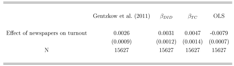
3.1 Eects of newspapers on electoral participation in the US
Gentzkow et al. (2011) study the eect of newspapers on electoral participation in the US. They estimate OLS regressions of the change in turnout between consecutive elections in countycon
election dummies and the change of the number of daily newspapers available in county c. In
column 2 of their Table 2, they nd that one additional newspaper increases turnout by 0.26 percentage points in US presidential elections from 1872 to 1928. Their regression specication is exactly equivalent to that studied in Theorem S1. We estimate the weightswgtb in this application,
and nd that treatment eects in 32% of county × election cells receive a negative weight, and
that negative weights sum up to -0.27. The validity of their coecient therefore relies on the assumption that the eect of newspapers on turnout is constant over time and across counties. To avoid relying on that assumption, we use a rst estimator inspired from the weighted sum of Wald-DIDs in the rst point of Theorem 4.1. As the authors include state-year eects in their specications, we slightly modify our estimator to also allow for dierential trends across states. Our estimator is obtained in ve steps. First, for each election the sets of counties
Gst, Git, and Gdt are respectively dened as counties where the number of newspapers remains
stable, increases, and decreases between elections t−1 and t. Second, we restrict the sample
to counties in Gst or Git and estimate a 2SLS regression of the change in turnout between
elections t − 1 and t on state dummies and the change in the number of newspapers. The
instrument for the change in newspapers is a dummy for counties inGit. LetβDID(1,0, t)denote
the coecient of the change in newspapers in this regression. Without the state dummies, we would have βDID(1,0, t) = WDID∗ (1,0, t). Therefore, βDID(1,0, t) is a modied version of WDID∗ (1,0, t) allowing for state-specic trends. Third, we restrict the sample to counties in Gst or Gdt and estimate a 2SLS regression of the change in turnout between elections t − 1
and t on state dummies and the change in the number of newspapers. The instrument for the
change in newspapers is a dummy for counties in Gdt. Here as well, the coecient of the change
in newspapers βDID(−1,0, t) is a modied version of WDID∗ (−1,0, t) allowing for state-specic
trends. Fourth, we estimate the weights wt and w10|t allowing for state-specic trends. We
repeat these steps for each election and our estimator is nally equal to
βDID =
16
X
t=0
This estimator does not rely on any constant treatment eect assumption, because it only uses counties where the number of newspapers is stable as controls.
However, this estimator still requires that the eect of newspapers on turnout do not vary over time (Assumption 4 in the main paper). In this context, this assumption is not warranted. Historians have shown that in the end of the 19th century, alternative ways of communicating information such as radio stations, telegraphic lines, and telephonic lines quickly developed in the US, thus ending the print monopoly of mass media (see White, 2003). This might have reduced the eects of newspapers. In their Table 5, the authors give suggestive evidence of this by showing that their regression coecients diminish over time. To avoid relying on that assumption, we use a second estimator βT C. βT C closely resembles the weighted sum of
Wald-TCs we introduced in the second point of Theorem 4.1, except that we allow for state-specic trends in each of the regressions we estimate to compute this weighted sum.67 On the
other end, estimating a Wald-CIC type of estimator while controlling for state-specic trends appears dicult. For each pairs of consecutive elections, there are many states where only few counties had, say, 2 newspapers at both elections. This makes it impossible to estimate the quantile-quantile transforms Qd within-state.8 We could estimate a weighted average of
Wald-CIC estimators without controlling for state-specic trends, but we prefer to remain as close as possible to the authors' original specication
Results are presented in Table 2 below. βDID is close to the estimator in Gentzkow et al.
(2011). On the other hand,βT C is almost twice as large and is signicantly dierent from their
estimator (t-stat=2.05). It is also signicantly dierent fromβDIDat the 10% level (t-stat=1.72).
To reconstruct the change in turnout that a county in Git or Gdt would have experienced if its
number of newspapers had not changed,βDID uses all counties in the same state and in Gst. To
reconstruct this counterfactual trend,βT C only uses counties in the same state, in Gst, and with
the same number of newspapers in period t−1 as the county in Git or Gdt. The fact that βT C
andβDID substantially dier indicates that among counties inGst, those with dierent numbers
of newspapers experience dierent evolutions of their turnouts. βDID and βT C rely on dierent
common trends assumptions between counties. But challenging one while defending the other seems dicult as these two assumptions are substantively very close. On the other hand, βT C
does not require that the eect of newspapers on turnout be constant over time, an assumption 6Using directly the two weighted sums we introduced in the rst and second points of Theorem 4.1 increases
even further the dierence between our estimators and that of Gentzkow et al. (2011).
7Only 18% of county×election cells have 3 newspapers or more, and only 9% have 4 or more. To estimate
the numerators of our Wald-TCs, we group the number of newspapers into 4 categories: 0, 1, 2, and more than 3. Results remain unchanged if we instead group the number of newspapers into 5 categories: 0, 1, 2, 3, and more than 4.
8On the other hand, this does not prevent us from estimating the additive shifts δd within-state, which we
which is not warranted in this context as we explained above. We therefore choose βT C as our
[image:22.612.62.538.142.276.2]preferred estimator.
Table S 2: Eect of one additional newspaper on turnout
Gentzkow et al. (2011) βDID βT C OLS
Eect of newspapers on turnout 0.0026 0.0031 0.0047 -0.0079
(0.0009) (0.0012) (0.0014) (0.0007)
N 15627 15627 15627 15627
Notes. This table reports estimates of the eect of one additional newspaper on turnout. Standard errors are clustered at the district level. ForβDID andβT C, clustered standard errors are obtained by block bootstrap.
This application also illustrates that our Wald-TC estimator can be used when only aggregate data are available, provided all units in each group × period cell share the same value of the
treatment, as is the case in Gentzkow et al. (2011). In such instances, our Wald-CIC estimator can also be used if one is ready to assume that Assumptions 1-2 and 6-7 are satised with Ygt
instead of Y. On the other hand, when units in the same group×period cell can have dierent
values of the treatment, one cannot use our Wald-TC and Wald-CIC estimators, becauseδdand Qd cannot be estimated from aggregate data. This is for instance the case in Enikolopov et al.
(2011). In such instances, authors can still follow our recommendation of nding a control group where treatment is stable and then estimate the Wald-DID.
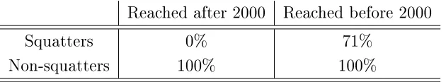
3.2 Eects of a titling program in Peru on labour supply
presents the share of households with a property title in 2000 in each group.
Table S 3: Share of households with a property right
Reached after 2000 Reached before 2000
Squatters 0% 71%
Non-squatters 100% 100%
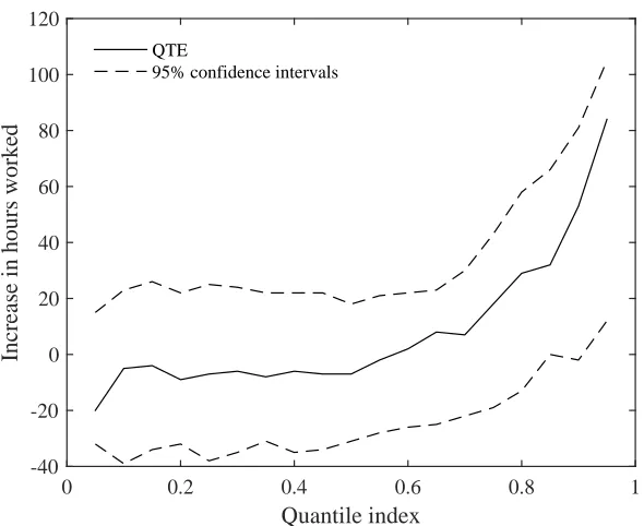
In Table 5 of her paper, the author uses 2SLS regressions to estimate the eect of having a property right on househods' labor supply. Her dependent variable is the number of hours worked per week by each household. Her explanatory variables are a dummy for squatters, a dummy for neighbourhoods reached before 2000, a dummy for whether the household has a property right, and a rich set of 62 control variables. Her instrument for property rights is the interaction of the squatters and reached before 2000 dummies. Therefore, her estimator is a Wald-DID accounting linearly for the eect of covariates. We revisit her results and compute instead the estimator cWCICX introduced in Section 5.2 of the main paper, with the same set of covariates. WcCICX also accounts linearly for the eect of covariates so this estimator is comparable to the author's. As all units in the control group are treated, we cannot estimate exactlyWcCICX but we follow Theorem 3.5 and apply the quantile-quantile transform of treated units in the control group to untreated units in the treatment group. On top of Assumptions 1X-2X and 6X-7X, the validity of this estimator also requires a conditional version of Assumption 10. Her Wald-DID and our Wald-CIC estimator with covariates are respectively equal to 18.07 and 16.17, thus implying that being granted a property title increases the number of hours worked by 16 to 18 hours. The two point estimates are not signicantly dierent (t-stat=1.29). Quantile treatment eects are shown in Figure 3. They are negative and insignicant in the bottom of the distribution of the outcome, and positive and signicant in the top. As per our estimates, being granted a property title decreases the rst decile of labour supply by 5 hours and increases the 9th decile by 53 hours. These two estimates are signicantly dierent (t-stat=2.21). The best ane approximation to the QTE function has a slope of 74.6 with a standard error of 25.8.9
Overall, our reanalysis yields a point estimate very similar to the author's for the average eect of property titles, but it also unveils an interesting pattern of heterogeneous eects along the distribution of the outcome.
9We estimate the standard error of this slope by bootstrap: in each bootstrap sample, we estimate the QTE
Quantile index
0 0.2 0.4 0.6 0.8 1
Increase in hours worked
-40 -20 0 20 40 60 80 100 120
QTE
[image:24.612.153.448.71.312.2]95% confidence intervals
Figure S3: Estimated LQTEs on the number of hours worked in Field (2005).
4 Supplementary proofs
In this section and in the next, we use the same notations as those used in the proofs of de Chaise-martin & D'Haultf÷uille (2015).
Theorem 3.3 (sharpness of the bounds)
Sharpness of the bounds for FY11(d)|S1(y)
We only consider the sharpness ofFCIC,0, the reasoning being similar for the upper bound. The
proof is also similar and actually simpler for d = 1. The corresponding bounds are proper cdf,
so we do not have to consider converging sequences of cdf as we do in case b) below.
a. λ00 > 1. We show that if Assumptions 2, 7, and 9 hold, then FCIC,0 is sharp. For that
purpose, we constructeh0,Ue0,Ve such that:
(i) Y =eh0(Ue0, T) when D= 0 and D= 1{Ve ≥vGT};
(ii) eh0(., t)is strictly increasing for t∈ {0,1};
(iv) Feh
0(Ue0,1)|G=0,T=1,Ve∈[v00,v01)=T0.
First, let
e
h0(.,0) = F000−1◦G0(T0)◦F
−1 001,
e
h0(.,1) = F001−1.
Second, let
e
U0 = (1−D)eh−01(Y, T)
+D(1−T)(1−G)1{V ∈[v00, v01)}Ue01
+DT G1{V ∈[v11, v00)}Ue02
+D[1−(1−T)(1−G)1{V ∈[v00, v01)} −T G1{V ∈[v11, v00)}]U0,
whereUe01 and Ue02 are two random variables such that S(Ue01) = S(Ue02) = (0,1), and
F e
U1
0|G=0,T=0,V∈[v00,v01) =T0◦F
−1 001,
FUe2
0|G=1,T=1,V∈[v11,v00) =C0(T0)◦F
−1 001.
F e
U1
0|G=0,T=0,V∈[v00,v01)is a valid cdf on(0,1)since (i)T0 is increasing by Assumption 9 andF
−1 001 is
also increasing, (ii) limy→yT0(y) = 0 and limy→yT0(y) = 1 when λ00 >1. FUe02|G=1,T=1,V∈[v11,v00)
is also a valid cdf on (0,1) since (i) C0(T0) is increasing by Assumption 9 and F
−1
001 is also
increasing, (ii) C0(T0) (S(Y)) = (0,1)when λ00 >1, as per the second point of Lemma S1.
Third, for every u∈(0,1), let
P0(u) = T0◦F
−1 001(u),
P1(u) = C0(T0)◦F
−1 001(u),
P2(u) = H0◦G0(T0)◦F
−1 001(u).
As shown in the proof of Lemma S6 (lower bound, case 2), Assumption 9 ensures that P0(u),
P1(u), and P2(u) are non dierentiable at only one point. Moreover, using the fact that
F001 =
1 λ00
G0(T0) +
1− 1 λ00
T0, (20)
H0◦G0(T0) =λ10F011+ (1−λ10)C0(T0), (21)
and T0,G(T0), and C0(T0) are increasing under Assumption 9, one can show that
0≤
1− 1 λ00
P00(u)≤1,
0≤ (1−λ10)P
0
1(u)
P0
2(u)
for any u at which P0(.), P1(.), and P2(.) are dierentiable, and P20(u) > 0. Then, let BS0 and
BS1 be two Bernoulli random variables such that for everyu∈(0,1),
P(BS0 = 1|Ue0 =u, D = 0, G= 0, T = 1) =
1− 1 λ00
P00(u),
P(BS1 = 1|Ue0 =u, D = 0, G= 1, T = 0) =
(1−λ10)P10(u)
P0
2(u)
,
with the convention that P(BS0 = 1|Ue0 = u, D = 0, G = 0, T = 1) and P(BS1 = 1|Ue0 =
u, D = 0, G = 1, T = 0) are equal to 0 at the point at which P0(u), P1(u), and P2(u) are
not dierentiable, and P(BS1 = 1|Ue0 = u, D = 0, G = 1, T = 0) = 0 when P
0
2(u) = 0. The
rst convention is innocuous as it applies to a 0 Lebesgue measure set. As we shall see later,
the second convention is also innocuous, because when P20(u) = 0, Equation (21) implies that P10(u) = 0 as well.
Finally, let
e
V = (1−D)(1−G)T hBS0Ve
1+ (1−B
S0)Ve
2i
+(1−D)G(1−T)hBS1Ve
3+ (1−B
S1)Ve
4i
+ (1−(1−D) [(1−G)T +G(1−T)])V,
whereVe1,Ve2,Ve3, and Ve4 are such that S(Ve1) =S(V)∩[v00, v01), S(Ve2) =S(V)∩(−∞, v00),
S(Ve3) =S(V)∩[v11, v00), S(Ve4) =S(V)∩(−∞, v11), and
fVe1|G=0,T=1,D=0,B
S0=1,Ue0(v|u) = fV|G=0,T=0,V∈[v00,v01),Ue0(v|u),
f e
V2|G=0,T=1,D=0,B
S0=0,Ue0(v|u) = fV|G=0,T=0,V <v00,Ue0(v|u),
fVe3|G=1,T=0,D=0,B
S1=1,Ue0(v|u) = fV|G=1,T=1,V∈[v11,v00),Ue0(v|u),
f e
V4|G=1,T=0,D=0,B
S1=0,Ue0(v|u) = fV|G=1,T=1,V <v11,Ue0(v|u).
We shall now show that(eh0(.,0),eh0(.,1),Ue0,Ve)satises (i), (ii), (iii), and (iv). By construction, Point (i) is satised. Moreover, it follows from Assumption 7 that eh0(.,1) is strictly increasing
on(0,1). Besides, G0(T0)◦F
−1
001 is strictly increasing on (0,1) and included between 0 and 1 as
shown in the rst point of Lemma S1. F000−1 is also strictly increasing on (0,1)by Assumption 7.
Therefore,eh0(.,0)is also strictly increasing on (0,1), and Point (ii) is satised.
Then, we check Point (iii). We show that it holds in the control group. For that purpose, we use Bayes law to write
f
e
U0,Ve|G=0,T=t(u, v)
= P(V < ve 01|G= 0, T =t)[P(V < ve 00|G= 0, T =t,V < ve 01)f
e
U0|G=0,T=t,V <ve 00(u)fVe|G=0,T=t,V <ve 00,Ue0(v|u)
+P(Ve ∈[v00, v01)|G= 0, T =t,V < ve 01)f
e
U0|G=0,T=t,Ve∈[v00,v01)(u)fVe|G=0,T=t,Ve∈[v00,v01),Ue0(v|u)]
+P(Ve ≥v01|G= 0, T =t)fUe
and we show that all elements in the right-hand side of the previous display are equal for t= 0
and t= 1.
We rst evaluate all of these quantities when T = 1. First, it follows from the denition of Ve that
P(V < ve 01|G= 0, T = 1) =p0|01. (23)
Then,
P(Ue0 ≤u|G= 0, T = 1,V < ve 01) = P(Ue0 ≤u|G= 0, T = 1, D = 0)
= P(eh−01(Y,1)≤u|G= 0, T = 1, D = 0)
= P(Y ≤F001−1(u)|G= 0, T = 1, D = 0) = u.
Therefore,
fUe
0|G=0,T=1,V <ve 01(u) = 1.
Then, we have, almost everywhere,
f e
U0,1{Ve∈[v00,v01)}|G=0,T=1,V <ve 01(u,1)
= P(Ve ∈[v00, v01)|G= 0, T = 1,V < ve 01,Ue0 =u)f
e
U0|G=0,T=1,V <ve 01(u)
= P(BS0 = 1|G= 0, T = 1, D = 0,Ue0 =u)
=
1− 1 λ00
P00(u). (24)
The second equality follows from the denition ofVe, and fromf
e
U0|G=0,T=1,V <ve 01(u) = 1. Equation
(24) and the fact that P00 is a density imply that
P(Ve ∈[v00, v01)|G= 0, T = 1,V < ve 01) = 1−
1 λ00
, (25)
f e
U0|G=0,T=1,Ve∈[v00,v01)(u) =P
0
0(u), (26)
and
P(V < ve 00|G= 0, T = 1,V < ve 01) =
1 λ00
, (27)
fUe
0|G=0,T=1,V <ve 00(u) =λ00−(λ00−1)P
0
0(u). (28)
Next, we have
fVe|G=0,T=1,Ve∈[v
00,v01),Ue0(v|u) = fVe1|G=0,T=1,D=0,BS
0=1,Ue0(v|u),
= fV|G=0,T=0,V∈[v
and
fVe|G=0,T=1,V <ve
00,Ue0(v|u) = fVe2|G=0,T=1,D=0,BS0=0,Ue0(v|u)
= fV|G=0,T=0,V <v
00,Ue0(v|u). (30)
Then, we evaluate all of these quantities whenT = 0. First, notice that
P(V < ve 01|G= 0, T = 0) = P(V < v01|G= 0, T = 0)
= P(V < v01|G= 0, T = 1)
= p0|01. (31)
The rst equality follows from the denition of Ve and the second from the fact V satises Assumption 1. One can use similar arguments to show that
P(Ve ∈[v00, v01)|G= 0, T = 0,V < ve 01) = 1−
1 λ00
, (32)
P(V < ve 00|G= 0, T = 0,V < ve 01) =
1 λ00
. (33)
Then, it follows from the denition ofVe and Ue0 that
f e
U0|G=0,T=0,Ve∈[v00,v01)(u) =fUe01|G=0,T=0,V∈[v00,v01)(u) =P
0
0(u). (34)
Next,
P(Ue0 ≤u|G= 0, T = 0,V < ve 00) = P(Ue0 ≤u|G= 0, T = 0, D = 0)
= P(eh−01(Y,0)≤u|G= 0, T = 0, D = 0)
= P(Y ≤F000−1◦G0(T0)◦F
−1
001(u)|G= 0, T = 0, D= 0)
= G0(T0)◦F
−1 001(u)
= λ00u−(λ00−1)P0(u),
where the last equality follows from (20). This implies that
fUe
0|G=0,T=0,V <ve 00(u) =λ00−(λ00−1)P
0
0(u). (35)
Then, it follows from the denition ofVe that
f e
V|G=0,T=0,Ve∈[v00,v01),Ue0(v|u) = fV|G=0,T=0,V∈[v00,v01),Ue0(v|u), (36)
fVe|G=0,T=0,V <ve
00,Ue0(v|u) = fV|G=0,T=0,V <v00,Ue0(v|u). (37)
Finally,
fUe
0,Ve|G=0,T=0,Ve≥v01(u, v) = fU0,V|G=0,T=0,V≥v01(u, v)
= fU0,V|G=0,T=1,V≥v01(u, v)
= fUe
where the rst and last equality follow from the denition of (Ue0,Ve), while the second equality follows from the fact (U0, V)satises Assumption 1.
Finally, combining Equation (22) with Equations (23) and (31), (25) and (32), (27) and (33), (26) and (34), (28) and (35), (29) and (36), (30) and (37), and (38), we get that
fUe
0,Ve|G=0,T=1(u, v) = fUe0,Ve|G=0,T=0(u, v).
This shows that (iii) holds in the control group. Showing that it also holds in the treatment group relies on a very similar reasoning, so we skip this part of the proof due to a concern for brevity.
b. λ00 < 1. The idea is similar as in the previous case. A dierence, however, is that when
λ00 < 1 and y = +∞, T0 is not a proper cdf, but a defective one, since limy→+∞T0(y) < 1.
As a result, we cannot dene a DGP such that Te0 = T0, However, by Lemma S2, there exists a sequence (Tk0)k of cdf such that Tk0 → T0, G0(Tk0) is an increasing bijection from S(Y) to
(0,1) and C0(Tk0) is increasing and onto (0,1). We can then construct a sequence of DGP
(ehk0(.,0),ehk0(.,1),Ue0k,Vek) such that Points (i) to (iii) listed above hold for everyk, and such that
e
Tk
0 = T
k
0. Since T
k
0(y) converges to T0(y) for every y in
◦
S(Y), we thus dene a sequence of
DGP such thatTe0k can be arbitrarily close to T0 on ◦
S(Y) for suciently largek. Since C0(.) is
continuous, this proves that FCIC,0 is sharp on
◦
S(Y).
In what follows, we exhibitehk0(.,0) and ehk0(.,1) satisfying (i), as well as distributions of Ue0k for all relevant subpopulations which are a) compatible with the data, b) satisfy (iii), and c) reach the bound. We do not not exhibit (Ue0k,Vek) as we did in the previous proof, to avoid repeating twice similar arguments.
Let
ehk0(.,1) =G0(Tk0)−1 ehk0(.,0) =F000−1
ehk0(.,1)is strictly increasing on(0,1)sinceG0(Tk0)is an increasing bijection on(0,1)as shown in Lemma S2. ehk0(.,0)is strictly increasing on (0,1)under Assumption 7. Therefore, (i) is veried. Let us consider rst the distribution of Ue0k among untreated observations in the control group in period 1. It follows from Bayes rule that
F e
Uk
0|G=0,T=1,V <ve 00 =λ00FUe0k|G=0,T=1,V <ve 01+ (1−λ00)FUe0k|G=0,T=1,Ve∈[v01,v00) (39)
Givenehk0(.,1), to haveTe0k =Tk0, we must have
FUek
0|G=0,T=1,Ve∈[v01,v00) =T
k
0 ◦G0(Tk0)
−1
This denes a valid cdf since Tk0 is a cdf and G0(Tk0)
−1 is increasing and onto S(Y). It can be
achieved by constructing Ve using an appropriate Bernoulli random variable to split untreated observations in the control group in period 0 between some for which Ve ∈ [v01, v00), and some
for which V < ve 01, exactly as we did for λ00 >1.
Givenehk0(.,1), and the fact ehk0(Ue0k,1) =Y for all observations such that G= 0, T = 1,V < ve 01,
a few computations yield
FUek
0|G=0,T=1,V <ve 01 =F001◦G0(T
k
0)
−1.
Plugging the last two equations into (39) nally yields FUek
0|G=0,T=1,V <ve 00 = I, where I denotes
the identity function on [0,1].
Now, let us turn to untreated observations in the control group in period 0. Given ehk0(.,0), and the fact ehk0(Ue0k,0) = Y for all observations such that G = 0, T = 0,V < ve 00, a few computations yieldFUek
0|G=0,T=0,V <ve 00 =I. SinceY(0) is not observed for observations such that
G= 0, T = 1,Ve ∈[v01, v00), the data does not impose any constraint on their U0, so we can set
FUek
0|G=0,T=0,Ve∈[v01,v00) =T
k
0 ◦G0(Tk0)
−1
.
Therefore, the distributions of Ue0k|G = 0, T = t,V < ve 01 and Ue0k|G = 0, T = t,Ve ∈ [v01, v00)
satisfy (iii).
Then, let us consider untreated observations in the treatment group in period 1. Using the denition ofehk0(.,1)and the factehk0(Ue0k,1) =Y for all observations such thatG= 1, T = 1,V <e
v11, one can show after a few computations that
F e
Uk
0|G=1,T=1,V <ve 11 =F011◦G0(T
k
0)
−1.
SinceY(0) is not observed for observations such thatG= 1, T = 1,Ve ∈[v11, v00), the data does not impose any constraint on their U0, so we can set
FUek
0|G=1,T=1,Ve∈[v11,v00)=C0(T
k
0)◦G0(Tk0)
−1.
This denes a valid cdf, as shown in Points 2 and 3 of Lemma S2.
Finally, let us consider untreated observations in the treatment group in period 0. It follows from Bayes rule that we must have
F e
Uk
0|G=1,T=0,V <ve 00 =λ10FUe0k|G=1,T=0,V <ve 11 + (1−λ10)FUe0k|G=1,T=0,Ve∈[v11,v00). (40)
To satisfy point (iii), we must have
FUek
0|G=1,T=0,V <ve 11 =F011◦G0(T
k
0)
−1
This can be achieved by constructingVe using an appropriate Bernoulli random variable to split untreated observations in the treatment group in period 0 between some for whichVe ∈[v11, v00),
and some for which V < ve 11, exactly as we did for λ00 >1. Using the denition of ehk0(.,1)and the factehk0(Ue0k,1) =Y for all observations such that G= 0, T = 1,V < ve 11, one can show after
a few computations that
FUek
0|G=1,T=0,V <ve 00 =F010◦F
−1 000.
Plugging the last two equations into (40) nally yields
FUek
0|G=1,T=0,Ve∈[v11,v00) =
p0|10F010◦F000−1−p0|11F011◦G0(Tk0)
−1
p0|10−p0|11
= C0(Tk0)◦G0(Tk0)
−1.
Therefore, the distributions of Ue0k|G = 1, T = t,V < ve 11 and Ue0k|G = 1, T = t,Ve ∈ [v11, v00) satisfy (iii). This completes the proof when λ00<1.
Sharpness of the bounds for ∆ and τq
We prove that the bounds on ∆ and τq are sharp under Assumption 9. We only focus on
the lower bound, the result being similar for the upper bound. The model and data impose no condition on the joint distribution of (U0, U1). Hence, by the previous sharpness proof we
can rationalize the fact that (FY11(0)|S1, FY11(1)|S1) = (FCIC,0, FCIC,1) when λ00 > 1. Sharpness
of ∆ and τq follows directly. When λ00 < 1, on the other hand, we can only rationalize the
fact that (FY11(0)|S1, FY11(1)|S1) = (C0k, FCIC,1), where C0k converges pointwise to FCIC,0. To
show the sharpness of the LATE and LQTE, we thus have to prove that limk→∞R ydC0k(y) =
R
ydFCIC,0(y) and limk→∞C0−k1(q) = F−CIC,1 0(q).
As for the LATE, we have, by integration by parts for Lebesgue-Stieljes integrals, Z
ydC0k(y) =y−
Z y
y
C0kdy=−
Z 0
y
C0k(y)dy+
Z y
0
[1−C0k(y)]dy. (41)
We now prove the convergence of each integral in the right-hand side. As shown by Lemma S2,
C0k can be dened as C0k = C0(Tk0) with T
k
0 ≤ T0, T0 denoting FY11(0)|S0. Because C0(T0) =
FY11(0)|S1 and C0(.) is increasing when λ00 < 1, C0k ≤ FY11(0)|S1. E(|Y11(0)| |S1) < +∞ implies
that R0
y FY11(0)|S1(y)dy <+∞. Thus, by the dominated convergence theorem,
lim k→∞
Z 0
y
C0kdy=
Z 0
y
FCIC,0(y)dy <+∞.
Now consider the second integral in (41). Ify <+∞, we can also apply the dominated
conver-gence theorem: 1−C0k ≤1implies that
Ry
0 [1−C0k(y)]dy→
Ry
0
1−FCIC,0(y)dy. Ify = +∞, limy→+∞FCIC,0(y) =` <1 so that
Z y
0