warwick.ac.uk/lib-publications
Original citation:Kosmidis, Ioannis. (2014) Bias in parametric estimation : reduction and useful side-effects. Wiley Interdisciplinary Reviews: Computational Statistics, 6 (3). pp. 185-196.
Permanent WRAP url:
http://wrap.warwick.ac.uk/98829
Copyright and reuse:
The Warwick Research Archive Portal (WRAP) makes this work of researchers of the University of Warwick available open access under the following conditions.
This article is made available under the Attribution-NonCommercial 3.0 Unported (CC BY-NC 3.0) license and may be reused according to the conditions of the license. For more details see: http://creativecommons.org/licenses/by-nc/3.0/
A note on versions:
The version presented in WRAP is the published version, or, version of record, and may be cited as it appears here.
Bias in parametric estimation:
reduction and useful side-effects
Ioannis Kosmidis
∗The bias of an estimator is defined as the difference of its expected value from the parameter to be estimated, where the expectation is with respect to the model. Loosely speaking, small bias reflects the desire that if an experiment is repeated indefinitely then the average of all the resultant estimates will be close to the parameter value that is estimated. The current article is a review of the still-expanding repository of methods that have been developed to reduce bias in the estimation of parametric models. The review provides a unifying framework where all those methods are seen as attempts to approximate the solution of a simple estimating equation. Of particular focus is the maximum likelihood estimator, which despite being asymptotically unbiased under the usual regularity conditions, has finite-sample bias that can result in significant loss of performance of standard inferential procedures. An informal comparison of the methods is made revealing some useful practical side-effects in the estimation of popular models in practice including: (1) shrinkage of the estimators in binomial and multinomial regression models that guarantees finiteness even in cases of data separation where the maximum likelihood estimator is infinite and (2) inferential benefits for models that require the estimation of dispersion or precision parameters.© 2014 The Authors.WIREs Computational Statisticspublished by Wiley Periodicals, Inc.
How to cite this article:
WIREs Comput Stat2014, 6:185–196. doi: 10.1002/wics.1296
Keywords: jackknife/bootstrap; indirect inference; penalized likelihood; infinite estimates; separation in models with categorical responses
∗Correspondence to: [email protected]
Department of Statistical Science, University College London, Lon-don, United Kingdom
Conflict of interest: The author has declared no conflicts of interest for this article.
Supplementary material for this article is available upon request and includes a script that reproduces the analyses of the gaso-line yield data using Beta regression models (wireGasogaso-line.R). The script for the wine tasting data case study with cumula-tive link models is available at the supplementary material of Kosmidis30 and can be obtained following the associated DOI
link in the References section. A change in behavior at the latest version of the ordinal R package at the time of writing (version 2013.9-30) returns nonavailable values for the earlier estimated standard errors, and Z-values for the parameters of cumulative link models when at least one infinite estimate is detected. For this reason, the wine data analyses can be reproduced using version 2012.01-19 of the ordinal package which is available for download at http://cran.r-project.org/src/contrib/Archive/ordinal/
IMPACT OF BIAS IN ESTIMATION
B
y its definition, bias necessarily depends on how the model is written in terms of its parameters and this dependence makes it not a strong statisti-cal principle in terms of evaluating the performance of estimators; e.g., unbiasedness of the familiar sam-ple varianceS2as an estimator of𝜎2does not deliveran unbiased estimator of𝜎itself. Despite this fact, an extensive amount of literature has focused on unbi-ased estimators (estimators with zero bias) as the basis of refined statistical procedures (e.g., finding minimum variance unbiased estimators). In such work unbi-asedness plays the dual role of a condition that (1) allows the restriction of the class of possible estima-tors in order to obtain something useful (like mini-mum variance amongst unbiased estimators), and (2) ensures that estimation is performed in an impartial
Volume 6, May/June 2014 185
way, ruling out estimators that would favour one or more parameter values at the cost of neglect-ing other possible values. Lehmann and Casella1
is a thorough review of statistical methods that are optimal once attention is restricted to unbiased estimators.
Another stream of literature has focused in reducing the bias of estimators, as a means to alleviat-ing the sometimes considerable problems that bias can cause in inference. This literature, despite dating back to the early years of statistical science, is resurfacing as increasingly relevant as the complexity of models used in practice increases and pushes traditional estimation methods to their theoretical limits.
The current review focuses on the latter litera-ture, explaining the link between the available meth-ods for bias reduction and their relative merits and disadvantages through the analysis of real data sets.
The following case study demonstrates the direct consequences that the bias in the estimation of a single nuisance (or incidental) parameter can have in inference, even if all parameters of interest are estimated with negligible bias.
Gasoline Yield Data
To demonstrate how bias can in some cases severely affect estimation and inference we follow the gaso-line yield data example in Kosmidis and Firth2 and
Grün et al.3 The gasoline yield data4 consists of
n=32 observations on the proportion of crude oil converted to gasoline after distillation and fraction-ation on 10 distinct experimental settings for the triplet (1) temperature in degrees Fahrenheit at which 10% of crude oil has vaporized, (2) crude oil grav-ity, and (3) vapor pressure of crude oil. The tem-perature at which all gasoline has vaporized is also recorded in degrees Fahrenheit for each one of the 32 observations.
The task is to fit a statistical model that links the proportion of crude oil converted to gasoline with the experimental settings and the temperature at which all gasoline has vaporized. For this we assume that the observed proportions of crude oil converted to gasoliney1,y2,…,ynare realizations of independent Beta distributed random variables Y1,…,Yn, where 𝜇i=E(Yi) and var(Yi)=𝜇i(1−𝜇i)/(1+𝜙). Hence, in
this parameterization, 𝜙 is a precision parameter (i=1,…,n). Then, the mean 𝜇i of the ith response can be linked to a linear combination of covariates and regression parameters via the logistic link function as
log 𝜇i
1−𝜇i =𝛼+ 9 ∑
t=1
𝛾tsit+𝛿ti (i=1,…,n). (1)
In the above expression,si1,…,si9are the values of nine dummy covariates which represent the 10 distinct experimental settings in the data set and ti
is the temperature in degrees Fahrenheit at which all gasoline has vaporized for the ith observation (i=1,…,n).
The parameters 𝜃=(𝛼,𝛾1, …,𝛾9,𝛿,𝜙) are esti-mated using maximum likelihood and the estiesti-mated standard errors for the estimates are calculated using the square roots of the diagonal elements of the inverse of the Fisher information matrix for model 1. The parameter𝜙 is considered here to be a nuisance (or incidental) parameter which is only estimated to com-plete the specification of the Beta regression model.
Table 1 shows the parameter estimates with the corresponding estimated standard errors and the 95% Wald-type confidence intervals. One immediate observation from the table of coefficients is the very large estimate for the precision parameter 𝜙. If this is merely the effect of upward bias then this bias will result in underestimation of the standard errors because for such a model the entries of the Fisher information matrix corresponding to the regression parameters𝛼,𝛾1,…,𝛾9,𝛿 are quantities of the form ‘𝜙times a function of𝜃’ (see Refs 2, 3 for expressions on the Fisher information). Hence, if the estimation of 𝜙 is prone to upward bias, then this can lead to confidence intervals that are shorter than expected at any specified nominal level and/or anti-conservative hypothesis testing procedures, which in turn result in spuriously strong conclusions.
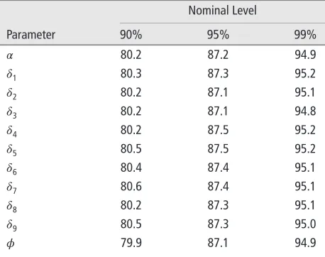
To check whether this is indeed the case a small simulation study has been designed where 50000 samples are simulated from the maximum likelihood fit shown in Table 1. Maximum likelihood is used to fit model 1 on each simulated sample and the bias of the maximum likelihood estimator is estimated using the resultant parameter estimates. The estimated bias for 𝛼is 0.010 while the estimated biases for𝛾1,…,𝛾9,𝛿 are all less than 0.005 in absolute value, providing indications that bias on the regression parameters is of no consequence. Nevertheless, the estimated bias for 𝜙is 299.779 which indicates a strong upward bias in the estimation of𝜙. To check how the upward bias in the precision parameter can affect the usual Wald-type inferences, we estimate the coverage probability (the probability that the confidence intervals contains the true parameter value) of the individual Wald-Type confidence intervals at levels 90, 95, and 99%. Table 2 shows the results. It is clear that the Wald-type confidence intervals systematically undercover the true parameter value across parameters.
TABLE 1 Maximum Likelihood Estimates for the Parameters of Model 1 with the Corresponding Estimated Standard Errors and the Wald-Type 95% Confidence Intervals (‘estimate’±1.96 ‘estimated standard error’).
Parameter Estimate Estimated Standard Error 95% Confidence Interval
𝛼 −6.160 0.182 −6.517 −5.802
𝛾1 1.728 0.101 1.529 1.926
𝛾2 1.323 0.118 1.092 1.554
𝛾3 1.572 0.116 1.345 1.800
𝛾4 1.060 0.102 0.859 1.260
𝛾5 1.134 0.104 0.931 1.337
𝛾6 1.040 0.106 0.832 1.248
𝛾7 0.544 0.109 0.330 0.758
𝛾8 0.496 0.109 0.282 0.709
𝛾9 0.386 0.119 0.153 0.618
𝛿 0.011 0.000 0.010 0.012
𝜙 440.278 110.026 224.632 655.925
TABLE 2 Estimated Coverage of Wald-Type Confidence Intervals at Nominal Level 90, 95, and 99%. Estimated Standard Errors Are Calculated Using the Fisher Information at the Maximum Likelihood Estimates.
Nominal Level
Parameter 90% 95% 99%
𝛼 80.2 87.2 94.9
𝛿1 80.3 87.3 95.2
𝛿2 80.2 87.1 95.1
𝛿3 80.2 87.1 94.8
𝛿4 80.2 87.5 95.2
𝛿5 80.5 87.5 95.2
𝛿6 80.4 87.4 95.1
𝛿7 80.6 87.4 95.1
𝛿8 80.2 87.3 95.1
𝛿9 80.5 87.3 95.0
𝜙 79.9 87.1 94.9
function, like logarithm (see e.g. Ref 3). More gen-erally, similar consequences of bias in inference are present in all exponential family models that involve the estimation of dispersion (or precision) parameters.
CONSISTENCY, BIAS, AND VARIANCE
Suppose that interest is in the estimation of ap-vector of parameters 𝜃, from data y(n) assumed
to be realizations of a random quantity y(n)
dis-tributed according to a parametric distribution M𝜃, 𝜃=(𝜃1,…,𝜃p)T∈ Θ⊂ℜp. The superscript n here is
used as an indication of the information in the data and is usually the sample size in the sense that the
realization ofY(n) isy(n)=(y
1, …,yn)T. An estimator
of𝜃 is a function ̂𝜃≡t(Y(n))and in the presence of data the estimate would bet(y(n)).
An estimator ̂𝜃=t(Y(n)) is consistent if it con-verges in probability to the unknown parameter𝜃 as
n→∞. Consistency is usually an essential requirement for a good estimator because given that the family of distributionsM𝜃 is large enough, it ensures that asn
increases the distribution of ̂𝜃becomes concentrated around the parameter𝜃, essentially providing a prac-tical reassurance that for very large n the estimator recovers𝜃.
The bias of an estimator is defined as
B(𝜃) =E𝜃(̂𝜃−𝜃 )
.
Loosely speaking, small bias reflects the desire that if an experiment that results in datay(n)is repeated
indefinitely, then the long-run average of all the resul-tant estimates will not be far from 𝜃. Small bias is a much weaker and hence less useful requirement than consistency. Indeed, one may get an inconsis-tent estimator with zero bias or a consisinconsis-tent estima-tor that is biased. For example, ifY(n)=(Y
1,…,Yn)T,
with Y1, …,Yn mutually independent random vari-ables with Yi~N(𝜇,𝜎2) then t(Y(n))=Y
1 is an
unbi-ased but inconsistent estimator of 𝜇. On the other hand,t(Y(n))=∑n
i=1Yi+1∕n is a consistent
estima-tor for𝜇but has biasB(t(Y(n)))=1/n. So, bias becomes
relevant only if it is accompanied by guarantees of con-sistency, or more generally when the variability ofV
around𝜃 is small (see Ref 5, § 8.1 for a discussion along this lines).
[image:4.594.69.298.337.518.2]estimator. The Cramér-Rao inequality states that the variance of any estimator̂𝜃(n)satisfies
var(̂𝜃(n))⪰{1
p+𝛻𝜃B(𝜃)}T{F(𝜃)}−1{1p+𝛻𝜃B(𝜃)}, (2) where 1p is the p×p identity matrix and the inequality A⪰C means that A−C is a positive semidefinite matrix. The matrix F(𝜃) is the Fisher (or expected) information matrix which is defined as
F(𝜃)=E𝜃{S(𝜃)S(𝜃)T}, where S(𝜃)=𝛻
𝜃l(𝜃) and l(𝜃) is the log-likelihood function for 𝜃. The Cramér-Rao inequality shows what is the ‘lowest’ attainable vari-ance for an estimator in terms of the derivatives of its bias and the Fisher information.
Maximum Likelihood Estimation
Denote f(y;𝜃) the joint density or probability mass function implied by the family of distributions M𝜃. The maximum likelihood estimator ̂𝜃 is the value of 𝜃 which maximizes the log-likelihood function
l(𝜃;y(n))=logf(y(n);𝜃). Given that the log-likelihood
function is sufficiently smooth on𝜃,̂𝜃can be obtained as the solution of the score equations
S(𝜃) =𝛻𝜃l(𝜃) =0,
provided that the observed information matrixI(𝜃) = −𝛻𝜃𝛻T𝜃l(𝜃)is positive definite when evaluated at̂𝜃. An appealing property of the maximum likelihood esti-mator is its invariance under one-to-one reparameter-izations of the model. If𝜃′=g(𝜃) for some one-to-one function g:ℜp→ℜp, then the maximum likelihood
estimator of𝜃′is simplyg(̂𝜃). This result states that when obtaining the maximum likelihood estimator of 𝜃, we automatically obtain the maximum likelihood estimator ofg(𝜃) for any functiongthat is one-to-one, simply by calculatingg(̂𝜃)without the need of max-imizing the likelihood ong(𝜃).
It can also be shown that the maximum likeli-hood estimator𝜃 has certain optimality properties if the ‘usual regularity conditions’ are satisfied. Infor-mally, the usual regularity conditions imply, among others, that (1)M𝜃 is identifiable (i.e.,M𝜃 ≠M𝜃′, for
any pair (𝜃,𝜃′) such that𝜃≠𝜃′, apart from sets of prob-ability zero), (2) p is finite, (3) that the parameter spaceΘdoes not depend on the sample space (which implies thatpdoes not depend onnand iv) that there exists a sufficient number of log-likelihood derivatives and expectations of those under M𝜃. A more tech-nical account of those conditions can be found in McCullagh6, § 7.1,7.2, or equivalently in Cox and
Hinkley5, §9.1.
If these conditions are satisfied, then̂𝜃is consis-tent and has bias of asymptotic orderO(n−1), which
means that its bias vanishes as n→∞. Moreover, the maximum likelihood estimator has the property that as n→∞ its distribution converges to a multi-variate Normal distribution with expectation 𝜃 and variance-covariance matrix {F(𝜃)}−1. Hence, the
vari-ance of the asymptotic distribution of the maximum likelihood estimator is exactly the Cramér-Rao lower bound {F(𝜃)}−1given in Eq. (2).
Reducing Bias
All the above shows that under the usual regularity conditions asn→∞, the maximum likelihood estima-tor ̂𝜃has optimal properties, a fact that makes it a default choice in applications. However, for finite n
these properties may deteriorate, in some cases causing severe problems in inference. Such an effect has been seen in the gasoline yield data case study where the bias of̂𝜃affects the performance of tests and the con-struction of confidence intervals based on the asymp-totic normality of̂𝜃.
Before reviewing the basic methods for reducing bias, it is necessary to emphasize again that bias neces-sarily depends on the parameterization of the model; if the bias of any estimator ̂𝜃 is reduced resulting to a less biased estimator ̃𝜃, then it is not necessary that the same will happen for the estimator g(̃𝜃).
In fact, the bias of the g(̃𝜃) as an estimator ofg(𝜃) may be considerably inflated. Hence, correction of the bias of the maximum likelihood estimator comes at the cost of destroying its invariance properties under reparameterization. Therefore, all the methods for bias reduction that are described in the current review should be seen with scepticism if invariance is a neces-sary requirement for the analysis. On the other hand if the parameterization is fixed by the problem or practi-tioner, one can do much better in terms of estimation and inference by reducing the bias. Furthermore, as it will be seen later, for some models reduction of bias produces useful side-effects which in many cases have motivated its routine use in applications. A thorough discussion on considerations on bias and variance and examples of exactly unbiased estimators that are useless or irrelevant can be found at Cox and Hinkley5§8.2 and Lehmann and Casella1§ 1.1.
BIAS REDUCTION—A SIMPLE RECIPE
WITH MANY DIFFERENT
IMPLEMENTATIONS
solution of the equation
̂𝜃−̃𝜃=B(𝜃), (3)
with respect to a new estimator ̃𝜃. Equation (3) is a moment-matching equation which links the proper-ties of the estimation method to the properproper-ties ofM𝜃
througĥ𝜃andB(𝜃), respectively. If both the function
B(𝜃) and 𝜃 were known then it is straightforward to show that ̃𝜃=̂𝜃−B(𝜃) has zero bias and hence, smaller mean squared error thañ𝜃. If, in addition, the initial estimator ̃𝜃has vanishing variance-covariance matrix asn→∞then an application of Chebyschev’s inequality shows that̃𝜃is consistent, even if ̃𝜃is not. Of course, if𝜃 is known then there is no reason for estimation, and furthermore, usually the functionB(𝜃) cannot be written in closed-form. The importance of Eq. (3) is that, despite of its limited practical value, all known methods to reduce bias can be usefully thought of as attempts to approximate its solution. These methods can be distinguished intoexplicitand
implicit.
EXPLICIT METHODS
Explicit methods rely on anone-stepprocedure where
B(𝜃) is estimated and then subtracted from̂𝜃resulting in the new estimator ̃𝜃. The most popular explicit methods for reducing bias are the jackknife, the boot-strap, and methods which use approximations of the bias function through asymptotic expansions ofB(𝜃).
Jackknife
For many common estimators including the maxi-mum likelihood estimator, the bias function can be expanded in decreasing powers ofnas
B(𝜃) = b(𝜃)
n +
b2(𝜃)
n2 +
b3(𝜃)
n3 +O
(
n−4), (4)
for an appropriate sequence of functions b(𝜃),b2(𝜃),
b3(𝜃), …, and so on, that are O(1) asn→∞.. From Eq. (4), the estimator ̂𝜃(−j) which results from leaving the jth random variable out of the original set of n
variables has the same bias expansion as in Eq. (4) but withnreplaced withn−1. In light of this observation, Quenouille7noticed that the estimator
̃𝜃=n̂𝜃− (n−1)𝜃,
where𝜃is the average of thenpossible leave-one-out estimators ̂𝜃(−1),…, ̂𝜃(−n), has bias expansion
−b2(𝜃)/n2+O(n−3) which is of smaller asymptotic
order than the O(n−1) bias of ̂𝜃. This procedure
is called jackknife (see Ref 8 for an overview of jackknife). Efron9 §2.3 shows the basic geometric
argument behind the jackknife; the jackknife is esti-mating the bias based on a linear extrapolation of the expected value of the estimator as a function of 1/n. The same procedure can be carried out for correcting bias in higher orders essentially replacing the linear extrapolation by quadratic extrapolation and so on. Schucany et al.10 give an elegant way of
deriving such higher order corrections in bias with the jackknife being a prominent special case of their method. The jackknife is an explicit method because the new estimator̂𝜃is simply
̃𝜃=̂𝜃−B(jack),
whereB(jack) = (n−1)(𝜃−̂𝜃)is the jackknife
estima-tor of the bias.
Bootstrap
Another class of popular explicit methods for the correction of the bias comes from the bootstrap frame-work. Bootstrap is a collection of methods that can be used to improve the accuracy of inference and operates under the principle that the ‘bootstrap sampleis for the sample, what the sample is for the population’. Then the same procedures that are applied on the sample can equally well be applied on the bootstrap sample giving direct access to estimated sampling distributions of statistics (see Ref 11 for an overview of bootstrap). The two dominant ways to obtain a bootstrap sample are (1) by sampling from the empirical distribution function (hence sampling with replacement from the original sample) giving rise to nonparametric boot-strap methods, and (2) by sampling from the fitted parametric model giving rise to parametric bootstrap methods. In all cases, the bias of an estimator can be estimated by B(boot) =𝜃∗−̂𝜃, where 𝜃∗ is the average of the estimates based on each of the boot-strap samples. Efron and Tibshirani12 and Davison
and Hinkley13 are thorough treatments of bootstrap
methodology. Under general conditions Hall and Martin14showed that, if̂𝜃has a bias ofO(n−1) which
can be consistently estimated, then the estimator
̃𝜃=̂𝜃−B(boot) =2̂𝜃−𝜃∗
hasO(n−2)bias.
Asymptotic Bias Correction
Another widely used class of explicit methods involves the approximation of B(𝜃) by b(̂𝜃)∕n which is the first-term in the right hand side of Eq. (4) evaluated at̂𝜃. Cox and Snell,15in their investigation of higher
order properties of residuals in general parametric models, derive an expression for the first-order bias term b(𝜃)/n in Eq. (4), when ̂𝜃 is the maximum likelihood estimator. That expression has sparked a still-active research stream in correcting the bias by using the estimator
̃𝜃=̂𝜃−b(̂𝜃)∕n.
Efron16showed that̃𝜃has bias of ordero(n−1) which
is of smaller order than the O(n−1) bias of the
maximum likelihood estimator and that the asymp-totic variance of any estimator with O(n−2) bias
is greater or equal to the asymptotic variance of ̃𝜃 (second-order efficiency). For the interested reader, Pace and Salvan17give a thorough discussion of those
properties.
Landmark studies in the literature for asymp-totic bias corrections are Cook et al.18 who
investi-gate correcting the bias in nonlinear regression models with Normal errors and Cordeiro and McCullagh19
who treat generalized linear models with interesting results on the shrinkage properties of the reduced-bias estimators in binomial regression models and an attractive implementation through one supplementary reweighted least squares iteration. Furthermore, Bot-ter and Cordeiro20 and Cordeiro and Toyama Udo21
extend the results in Cordeiro and McCullagh19and
derive the first-order biases for generalized linear and nonlinear models with dispersion covariates.
The general form of the first-order bias term of the maximum likelihood estimator can be found in matrix form in Kosmidis and Firth22. Specifically,
b(𝜃)
n = − {F(𝜃)}
−1A (𝜃),
where A(𝜃) is a p-dimensional vector with compo-nents
At(𝜃) =1
2tr
[
{F(𝜃)}−1{Pt(𝜃) +Qt(𝜃)}](t=1,…,p),
(5) and where
Pt(𝜃) =E𝜃{S(𝜃)ST(𝜃)St(𝜃)} (t=1,…,p),
Qt(𝜃) = −E𝜃{I(𝜃)St(𝜃)} (t=1,…,p),
are higher order joint null moments of the gra-dient and the matrix of second derivatives of the log-likelihood.
Breslow and Lin23derive the expressions for the
asymptotic biases in generalized linear mixed models for various estimation methods and used those to correct for the bias. Higher order corrections have also appeared in the literature24 where expressions
for b(𝜃)/n+b2(𝜃)/n2 in Eq. (4) are obtained. The
expressions involved for such higher order corrections are too cumbersome requiring enormous effort in derivation and implementation, and there is always the danger that the benefits in estimation from this effort are only marginal, if any, compared to methods that are based on simply removing the first-order bias term.
Advantages and Disadvantages of Explicit
Methods
The main advantage of all explicit methods is the simplicity of their application. Once an estimate of bias is available, reduction of bias is simply a matter of an one-step procedure where the estimated bias is subtracted from the estimates. Nevertheless because of their explicit dependence on ̂𝜃, explicit methods directly inherit any of the instabilities of the original estimator. Such cases involve models with categorical responses where there is a positive probability that the maximum likelihood estimator is not finite (see Ref 25 for conditions that characterize when infinite estimates occur in multinomial response models) and have been the subject of study in works like Mehrabi and Matthews,26Heinze and Schemper,27Bull et al.,28
Kosmidis and Firth,29 Kosmidis and Firth,2 and
Kosmidis.30 In particular, Kosmidis30 relates to the
case study of the proportional odds models, discussed below.
Furthermore, asymptotic bias correction meth-ods have the disadvantage that are only applicable whenb(𝜃)/ncan be obtained in closed-form, which can be a tedious or even impractical task for many models (see, e.g., Ref 3 where the expressions for b(𝜃)/n are given for Beta regression models).
IMPLICIT METHODS
Implicit methods approximateB(𝜃) at the target esti-mator ̃𝜃 and then solve Eq. (3) with respect to ̃𝜃. Hence,̃𝜃is the solution of an implicit equation.
Indirect Inference
Gourieroux et al.31and can be used for bias reduction.
The simplest approach to bias reduction via indirect inference attempts to solve the equation
̃𝜃=̂𝜃−B(̃𝜃),
by approximatingB(𝜃) at̃𝜃through parametric boot-strap. Kuk32 independently produced the same idea
for reducing the bias in the estimation of general-ized linear models with random effects and Jiang and Turnbull33 give a comprehensive review of indirect
inference from a statistical point of view. Furthermore, Gourieroux et al.34and Phillips35discuss bias
reduc-tion through indirect inference in econometric appli-cations. Pfeffermann and Correa36give an alternative
approach to bias reduction which is in line with the basic idea of indirect inference.
Bias-Reducing Adjusted Score Equations
For the case where ̂𝜃 is the maximum likelihood estimator and under the usual regularity conditions, Firth37 and Kosmidis and Firth29 investigate whatpenalties need to be added toS(𝜃) in order to get an estimator that has asymptotically smaller bias than that of the maximum likelihood estimator. In its simplest form such an approach requires finding ̃𝜃by solving the adjusted score equations
S(̃𝜃)+A(̃𝜃)=0, (6)
with A(𝜃) as given in Eq. (5). Then ̃𝜃is an estimator witho(n−1)bias. Equation 6 can be rewritten as
{
F(̃𝜃)}−1S(̃𝜃)=
b(̃𝜃)
n ,
which reveals that ̃𝜃is another approximate solution to Eq. (3) because b(𝜃) ∕n approximates B(𝜃)up to orderO(n−2) and {F(𝜃)}−1S(𝜃) is theO(n−1/2) term in
the asymptotic expansion of̂𝜃−𝜃evaluated at𝜃∶=̃𝜃.
An important property of the estimator based on adjusted score functions, which is also shared by the estimator from asymptotic bias correction, is that it has the same asymptotic distribution as the maximum likelihood estimator, namely a Normal distribution centered at the true parameter value with variance-covariance matrix the Cramér-Rao lower bound {F(𝜃)}−1. Hence, the first-order methods that
are used for the maximum likelihood estimator, like Wald-type confidence intervals, score tests for model
comparison, and so on, are unaltered in their form and apply directly by using the new estimators.
It is noteworthy that in the case of full expo-nential families (e.g., logistic regression and Poisson log-linear models) the solution of Eq. (6) can be obtained by direct maximization of a penalized likeli-hood where the penalty is the Jeffreys38invariant prior
(see Ref 37 for details). It should also be stressed that not all models admit a penalized likelihood interpre-tation of bias reduction via adjusted scores. Kosmidis and Firth29give an easy-to-check necessary and
suffi-cient condition that identifies which univariate gener-alized linear models admit such pengener-alized likelihood interpretation and provide the form of the resultant penalties when the condition holds. That condition is a restriction on the variance function of the responses in terms of the derivative of the chosen link function.
Advantages and Disadvantages
The main disadvantage of implicit methods is that their application requires the solution of a set of implicit equations which in most of the useful cases requires numerical optimization. This task is even more computationally demanding for indirect infer-ence approaches in general models because of the necessity to approximate the bias function in a
p-dimensional space. Furthermore, indirect inference approaches inherit the disadvantages of explicit meth-ods because they explicitly depend on the original esti-mator.
The approach in Firth37 and Kosmidis and
Firth,29 on the other hand, does not directly depend
on̂𝜃and hence has gained considerable attention com-pared to the other approaches. Another reason for the considerable adaptation of this method are recent advances which simplify application through either iterated first-order bias adjustments (see Refs 3, 22) or iterated maximum likelihood fits on pseudo obser-vations (see Refs 2, 29, 30). Of course, as for the asymptotic bias correction methods the adjusted score equation approach to bias reduction has the disadvan-tage of being directly applicable only under the same conditions that guarantee the good limiting behav-ior of the maximum likelihood estimator and only when the score functions, Fisher information and the first-order bias term of the maximum likelihood esti-mator are available in closed-form.
PROPORTIONAL ODDS MODELS
This example was analyzed in Kosmidis.30 The data
set in Table 3 is from Randall39 and concerns a
TABLE 3 The Wine Tasting Data (Randall39).
Bitterness Scale
Temperature Contact 1 2 3 4 5
Cold No 4 9 5 0 0
Cold Yes 1 7 8 2 0
Warm No 0 5 8 3 2
Warm Yes 0 1 5 7 5
affect the bitterness of white wine. There are two factors in the experiment, temperature at the time of crushing the grapes (with two levels, ‘cold’ and ‘warm’) and contact of the juice with the skin (with two levels ‘Yes’ and ‘No’). For each combination of factors two bottles were rated on their bitterness by a panel of nine judges. The responses of the judges on the bitterness of the wine were taken on a continuous scale in the interval from 0 (‘None’) to 100 (‘Intense’) and then they were grouped correspondingly into five ordered categories, 1, 2, 3, 4, 5.
The task of the analysis is to test whether there are departures from the assumption of proportional odds. For performing such a test we use the more general partial proportional odds model of Peterson et al.40with
log 𝛾rs
1−𝛾rs=𝛼s−𝛽swr−𝜃zr (r=1,…,4;s=1,…,4),
(7) where wr and zr are dummy variables represent-ing the factors temperature and contact, respectively, 𝛼1,𝛼2,𝛼3𝛼4,𝛽1,𝛽2,𝛽3,𝛽4,𝜃are model parameters and 𝛾rs is the cumulative probability for the sth category
at the rth combination of levels for temperature and contact. Then we can check for departures from the proportional odds assumption by testing the hypoth-esis𝛽1=𝛽2=𝛽3=𝛽4, effectively comparing Eq. (7) to the proportional odds nested model that is implied by the hypothesis.
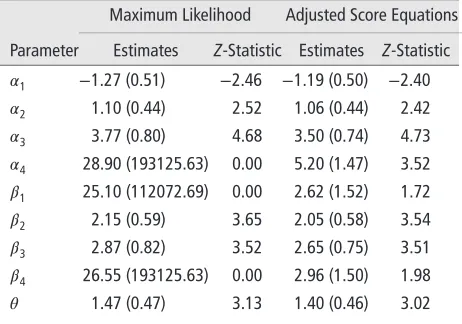
Table 4 shows the maximum likelihood mates for model Eq. (7) and the corresponding esti-mated standard errors as reported by the clm func-tion of the R package ordinal.41It is directly apparent
[image:9.594.297.528.140.302.2]that the absolute value of the estimates and estimated standard errors for the parameters 𝛼4, 𝛽1 and 𝛽4 is very large. Actually, these would diverge to infinity as the stopping criteria of the iterative fitting proce-dure used become stricter and the number of allowed iterations increases. The estimates for the remaining parameters are all finite and will preserve the value shown in Table 4 even if the number of allowed iter-ations increases. This is an instance of the problems
TABLE 4 The Maximum Likelihood and the Reduced-Bias Estimates for the Parameters of Model (7), the Corresponding Estimated Standard Errors (in parenthesis) and the Values of the CorrespondingZ-Statistic for the Hypothesis that the Corresponding Parameter is zero. The Maximum Likelihood Estimates andZ-statistics are as Reported by the clm R Package Ordinal41.
Maximum Likelihood Adjusted Score Equations
Parameter Estimates Z-Statistic Estimates Z-Statistic
𝛼1 −1.27 (0.51) −2.46 −1.19 (0.50) −2.40
𝛼2 1.10 (0.44) 2.52 1.06 (0.44) 2.42
𝛼3 3.77 (0.80) 4.68 3.50 (0.74) 4.73
𝛼4 28.90 (193125.63) 0.00 5.20 (1.47) 3.52
𝛽1 25.10 (112072.69) 0.00 2.62 (1.52) 1.72
𝛽2 2.15 (0.59) 3.65 2.05 (0.58) 3.54
𝛽3 2.87 (0.82) 3.52 2.65 (0.75) 3.51
𝛽4 26.55 (193125.63) 0.00 2.96 (1.50) 1.98
𝜃 1.47 (0.47) 3.13 1.40 (0.46) 3.02
that practitioners may face when dealing with categor-ical response models. Using a Wald-type statistic based on the maximum likelihood estimator for testing the hypothesis of proportional odds would be adventur-ous here because such a statistic explicitly depends on the estimates of 𝛽1, 𝛽2, 𝛽3 and 𝛽4. Of course, given that the likelihood is close to its maximal value at the estimates in Table 3, a likelihood ratio test can be used instead; the likelihood ratio test for this particular example has been carried out in Christensen.42
Note here that methods like the bootstrap and jackknife would require special considerations for their application in a well-designed experiment like the above, the question to be answered being what comprises an observation to be resampled or left-out. Even if such considerations were resolved, bootstrap and jackknife would be prone to the problem of infinite estimates. The latter is also true for the estimator based on asymptotic bias corrections and for indirect inference.
Kosmidis30derives the adjusted score equations
for cumulative link models, and uses them to cal-culate the reduced-bias estimates shown in the right of Table 4. The reduced-bias estimates based on the adjusted score functions are finite and, through the asymptotic normality of the reduced-bias estimator, they can form the basis of a Wald-test for the hypoth-esis𝛽1=𝛽2=𝛽3=𝛽4. This test has been carried out in Kosmidis30and gives ap-value of 0.861, providing no
evidence against the hypothesis of proportional odds. Furthermore, the values of the Z-statistics for 𝛼4, 𝛽1 and 𝛽4 in Table 4 are essentially zero when
typical behavior when the estimates diverge to infinity and it happens because the estimated standard errors diverge much faster than the estimates, irrespective of whether or not there is evidence against the individual hypotheses. This is also true if we were testing indi-vidual hypothesis at values other than zero, and can lead to invalid conclusions if the maximum likelihood output is interpreted naively; as shown in Table 4, the
Z-statistics based on the reduced-bias estimates are far from being zero.
Such inferential pitfalls with the use of the max-imum likelihood estimator are not specific to partial proportional odds models. For most models for cat-egorical and discrete data (binomial-response models like the logistic regression, multinomial response mod-els, Poisson log-linear modmod-els, and so on) there is a positive probability of infinite estimates. Bias reduc-tion through adjusted score funcreduc-tions has been found to provide a solution to those problems and the cor-responding methodology is quickly gaining in popu-larity and has found its way to commercial software like Stata and SAS. Open-source solutions include the logistf R package43 for logistic regressions which is
based on the work in Heinze and Schemper,27 the
pmlr R package44for multinomial logistic regressions
based on the work of Bull et al.28 and the brglm R
package45,46 which at the time of writing handles all
binomial-response models. At the time of writing, the brglm R package is being extended for the next major update which will handle all generalized linear models, including multinomial logistic regression2and ordinal
response models.30
GASOLINE YIELD DATA REVISITED
In this section, the reduced-bias estimates for the parameters of model 1 are calculated using jack-knife, bootstrap, asymptotic bias correction, and the approach of bias-reducing adjusted score functions. The full parametric bootstrap estimate of the bias has been obtained in our earlier treatment showing that the bias on the regression parameters is of no consequence. A fully nonparametric bootstrap where the bootstrap samples are produced by sub-sampling with replacement the full response-covariate com-binations (yi,si1,…,si9,ti) (i=1,…,n) is not advis-able here because the 9 dummy variadvis-ables si1,…,si9are representing 10 distinct experimental settings and sub-sampling those will result in singular fits with high probability (see also Ref 13, § 6.3 for a description of such problems in the simpler case of multiple lin-ear regression). An intermediate sub-sampling strategy is to resample residuals and use them with the orig-inal model matrix to get samples for the response.
This strategy lies between fully nonparametric boot-strap and fully parametric bootboot-strap (see Ref 13, § 7). Residual resampling works well in multiple linear regression because the response is related linearly to the regression parameters, which is not true for Beta regression. For more complicated models like general-ized linear models and Beta regression, an appropri-ate residual definition has to be chosen. Because Beta responses are restricted in (0,1), the best option is to resample residuals on the scale of the linear predictor and then transform back to the response scale using the inverse of the logistic link, obtaining bootstrap samples for the response (see Ref 13 expression (7.13) for rationale and implementation). In the current case we choose the ‘standardized weighted residual 2’ of Espinheira et al.47 because it appears to be the one
that is least sensitive to the inherent skewness of the response.
The reduced-bias estimates of 𝜙 using jack-knife, residual-resampling bootstrap (with 9999 bootstrap samples), asymptotic bias correction and bias-reducing adjusted score functions are 165.682, 236.003, 261.206, and 261.038, respectively, all indi-cating that the maximum likelihood estimator of 𝜙 is prone to substantial upward bias. The simulations in Kosmidis and Firth22 illustrate that asymptotic
bias correction and the bias-reducing adjusted score functions, correctly inflate the estimated standard errors to the extent that almost the exact coverage of the first-order Wald-type confidence intervals is recovered.
DISCUSSION AND CONCLUSION
As can be seen from the earlier case-studies, reduced-bias estimators can form the basis of asymptotic inferential procedures that have better performance than the corresponding procedures based on the initial estimator. Heinze and Schemper,27
Bull et al.,48 Kosmidis,49 Kosmidis and Firth,22,29
and Grün et al.3 all demonstrate that such improved
procedures are delivered either by using the penalized likelihood that results from the approximation of Eq. (3), or by replacing the initial estimator with the reduced-bias estimator in Wald-type pivots, as was done in the case-studies of this review.
At the time of writing the current review there is no general answer to which of the methods that have been reviewed here produces better results. All meth-ods deliver estimators that have o(n−1) bias which
is asymptotically smaller than the O(n−1) bias of
reduction approaches because the resultant estimates appear to be always finite, even in cases where the maximum likelihood estimates are infinite (see, e.g., Refs 27, 48, 29, 2, 30 for generalized linear and non-linear models with binomial, multinomial, and Pois-son responses). This has led researchers to promoting the routine use of the adjusted score equations in such models as an improved alternative to maximum like-lihood.
The general use, though, of the adjusted score equations approach is limited by its dependence on a closed-form expression for the first-order bias of the maximum likelihood estimator which may not be readily available or even intractable (e.g., generalized linear mixed effects models).
At this point, we should also stress that improv-ing bias does not always have desirable effects; an improvement in bias can sometimes result in infla-tion of the mean squared error, through an inflainfla-tion in the estimator’s variance. The use of simple simula-tion studies, similar to the one in Kosmidis and Firth22
is recommended for checking whether that is the case. If that is the case then the use of reduced-bias estimates in test statistics and confidence intervals is not recom-mended.
Furthermore, bias is a parameterization-specific quantity and any attempt to improve it will violate
the invariance properties of the maximum likelihood estimator. Hence, bias-reduction methods should be used with care, unless the parameterization is fixed either by the context or by the practitioner.
All the discussion in the current review has focused on the effect that bias can have and the bene-fits of its reduction in cases where the usual regularity conditions are satisfied. An important research avenue is the reduction of bias under departures from the reg-ularity conditions and especially when the dimension of the parameter space increases with the sample size. Lancaster50 gives a review of the issues that
econo-metricians and applied statisticians face in such set-tings. A viable route toward reduction of bias in such cases comes from the use of modified profile likelihood methods (see, Ref 51 for a brief introduction), which have been successfully used for reducing the bias in the estimation of dynamic panel data models in Bartolucci et al.52Another route is the appropriate adaptation of
indirect inference approaches or of other approximate solutions of Eq. (3) in such settings. The Econometric community is currently active in this direction, with a recent example being Gouriéroux et al.53where
indi-rect inference is applied to dynamic panel data models. These early attempts are only indicative that, there is still much to be explored and much work to be done on the topic of bias reduction in parametric estimation.
ACKNOWLEDGMENTS
The author thanks the Editor, the Review Editor, and three anonymous Referees for detailed, helpful comments which have substantially improved the presentation.
REFERENCES
1. Lehmann EL, Casella G. Theory of Point Estimation. 2nd ed. New York: Springer; 1998.
2. Kosmidis I, Firth D. Multinomial logit bias reduction
via the poisson log-linear model. Biometrika 2011,
98:755–759.
3. Grün B, Kosmidis I, Zeileis A. Extended𝛽 regression
in R: Shaken, stirred, mixed, and partitioned.J Statist
Softw2012, 48:1–25.
4. Prater NH. Estimate gasoline yields from crudes.
Petroleum Refiner1956, 35:236–238.
5. Cox DR, Hinkley DV.Theoretical Statistics. London:
Chapman & Hall Ltd.; 1974.
6. McCullagh P. Tensor Methods in Statistics. London:
Chapman and Hall; 1987.
7. Quenouille MH. Notes on bias in estimation.
Biometrika1956, 43:353–360.
8. Chernick MR. The jackknife: a resampling method with
connections to the bootstrap. Wiley Interdiscip Rev
Comput Stat2012, 4:224–226.
9. Efron B.The Jackknife, the Bootstrap and Other
Resam-pling Plans. Philadelphia, PA: SIAM [Society for Indus-trial and Applied Mathematics]; 1982.
10. Schucany WR, Gray HL, Owen DB. On bias reduction
in estimation.J Am Stat Assoc1971, 66:524–533.
11. Hesterberg T. Bootstrap.Wiley Interdiscip Rev Comput
Stat2011, 3:497–526.
12. Efron B, Tibshirani R.An Introduction to the Bootstrap.
New York: Chapman & Hall Ltd; 1993.
13. Davison AC, Hinkley DV.Bootstrap Methods and Their
14. Hall P, Martin MA. Exact convergence rate of bootstrap
quantile variance estimator. Probab Theory Rel Fields
1988, 80:261–268.
15. Cox DR, Snell EJ. A general definition of residuals (with
discussion). J Roy Statist Soc Ser B Methodol 1968,
30:248–275.
16. Efron B. Defining the curvature of a statistical problem (with applications to second order efficiency) (with
discussion).Ann Stat1975, 3:1189–1217.
17. Pace L, Salvan A. Principles of Statistical Inference:
From a Neo-Fisherian Perspective. London: World Sci-entific; 1997.
18. Cook RD, Tsai C-L, Wei BC. Bias in nonlinear
regres-sion.Biometrika1986, 73:615–623.
19. Cordeiro GM, McCullagh P. Bias correction in
gener-alized linear models.J Roy Statist Soc Ser B Methodol
1991, 53:629–643.
20. Botter DA, Cordeiro G. Improved estimators for
gen-eralized linear models with dispersion covariates.J Stat
Comput Simul1998, 62:91–104.
21. Cordeiro G, Toyama Udo M. Bias correction in
general-ized nonlinear models with dispersion covariates.
Com-mun Stat Theory Methods2008, 37:2219–225. 22. Kosmidis I, Firth D. A generic algorithm for reducing
bias in parametric estimation. Electron J Stat 2010,
4:1097–1112.
23. Breslow NE, Lin X. Bias correction in generalised linear mixed models with a single component of dispersion.
Biometrika1995, 82:81–91.
24. Cordeiro G, Barroso L. A third-order bias corrected
esti-mate in generalized linear models.Test2007, 16:76–89.
25. Albert A, Anderson J. On the existence of maxi-mum likelihood estimates in logistic regression models.
Biometrika1984, 71:1–10.
26. Mehrabi Y, Matthews JNS. Likelihood-based methods
for bias reduction in limiting dilution assays.Biometrics
1995, 51:1543–1549.
27. Heinze G, Schemper M. A solution to the problem
of separation in logistic regression. Stat Med 2002,
21:2409–2419.
28. Bull SB, Mak C, Greenwood C. A modified score function estimator for multinomial logistic regression
in small samples. Comput Stat Data Anal 2002, 39:
57–74.
29. Kosmidis I, Firth D. Bias reduction in exponential family
nonlinear models.Biometrika2009, 96:793–804.
30. Kosmidis I. Improved estimation in
cumu-lative link models. J Roy Stat Soc Ser B
2013b. doi:10.1111/rssb.12025. ArXiv e-prints.
arXiv:1204.0105v3 [stat.ME].
31. Gourieroux C, Monfort A, Renault E. Indirect
infer-ence.J Appl Econom1993, 8S:85–118.
32. Kuk AYC. Asymptotically unbiased estimation in
gener-alized linear models with random effects.J Roy Statist
Soc Ser B Methodol1995, 57:395–407.
33. Jiang W, Turnbull B. The indirect method: infer-ence based on intermediate statistics – synthesis and
examples.Statist Sci2004, 19:239–263.
34. Gourieroux C, Renault E, Touzi N. Chapter 13: Cal-ibration by simulation for small sample bias correc-tion. In: Mariano R, Schuermann T, Weeks MJ, eds.
Simulation-based Inference in Econometrics: Methods and Applications. 1st ed. Cambridge: Cambridge Uni-versity Press; 2000, 328–358.
35. Phillips PCB. Folklore theorems, implicit maps,
and indirect inference. Econometrica 2012, 80:
425–454.
36. Pfeffermann D, Correa S. Empirical bootstrap bias correction and estimation of prediction mean square
error in small area estimation. Biometrika 2012, 99:
457–472.
37. Firth D. Bias reduction of maximum likelihood
esti-mates.Biometrika1993, 80:27–38.
38. Jeffreys H. An invariant form for the prior probability
in estimation problems. Proc Roy Soc Lond 1946,
186:453–461.
39. Randall J. The analysis of sensory data by generalised
linear model.Biom J1989, 7:781–793.
40. Peterson B, Harrell J, Frank E. Partial proportional odds
models for ordinal response variables.Appl Stat1990,
39:205–217.
41. Christensen RHB.Ordinal—regression models for
ordi-nal data. R package version 2012.01-19; 2012b. Avail-able at: http://cran.r-project.org/src/contrib/Archive/ ordinal/. (Accessed September 20, 2013).
42. Christensen RHB.Ordinal—a tutorial on fitting
cumu-lative link models with the ordinal package. R package version 2012.01-19; 2012a. Available at: http://cran.
r-project.org/src/contrib/Archive/ordinal/. (Accessed
September 20, 2013).
43. Heinze G, Ploner M, Dunkler D, Southworth H.Logistf:
Firth’s bias reduced logistic regression. R package ver-sion 1.21; 2013.
44. Colby S, Lee S, Lewinger JP, Bull S.Pmlr: Penalized
Multinomial Logistic Regression. R package version 1.0; 2010.
45. Kosmidis I. On iterative adjustment of responses for
the reduction of bias in binary regression models. Technical Report 09-36. CRiSM working paper series; 2009.
46. Kosmidis I. brglm: Bias reduction in binary-response
Generalized Linear Models. R package version 0.5-9; 2013a.
47. Espinheira PL, Ferrari SLP, Cribari-Neto F. On
𝛽 regression residuals. J Appl Stat 2008, 35:
407–419.
48. Bull SB, Lewinger JB, Lee SSF. Confidence intervals for
multinomial logistic regression in sparse data.Stat Med
49. Kosmidis I. Bias reduction in exponential family non-linear models. Ph.D. thesis, Department of Statistics, University of Warwick; 2007.
50. Lancaster T. The incidental parameter problem since
1948.J Econom2000, 95:391–413.
51. Reid N. Likelihood inference. Wiley Interdiscip Rev
Comput Stat2010, 2:517–525.
52. Bartolucci F, Bellio R, Salvan A, Sartori N. Mod-ified profile likelihood for panel data models. Technical report. Available at SSRN repository; 2012.
53. Gouriéroux C, Phillips PCB, Yu J. Indirect inference
for dynamic panel models. J Econom 2010, 157: