An economic network in Nonth America

Munich Personal RePEc Archive

An economic network in North America

AROCHE REYES, FIDEL and MARQUEZ MENDOZA,

MARCO ANTONIO

UNIVERSIDAD NACIONAL AUTÓNOMA DE MÉXICO

2012

Online at

https://mpra.ub.uni-muenchen.de/61391/

1

An Economic Network in North America

Fidel Aroche Reyes Marco Antonio Marquez Mendoza

Abstract: Economic structures can be studied as networks of industries linked through flows of commodities that - in turn - the consuming sectors use as inputs. The Input-Output (IO) model is a suitable framework for analysing those structures, because its main target is the study of interdependence between sectors. In this paper we use a North American multi-region IO table in order to identify an economic regional network that results from a subset of the links between sectors in the countries involved. Those are defined by the exchange of goods between industries. Further, a density measure is used as an indicator of the network complexity, explained by the integration level and shape between those economies. Our results show that the US is by far the most integrated economy in North America; it also determines the shape of the network structure. In contrast, Canada and Mexico maintain scarce direct relationships.

Keywords: Economic structure, economic network, Input-Output model, North America

2

An Economic Network in North America

Qualitative Input-Output Analysis (QIOA) has been often employed to study economic structures; this methodology has yielded deep insights on the way industries interact within an economy (Czamanski and Ablas, 1979; Huriot, 1974; Campbell; 1975, Holub and Schnabl, 1985; Aroche, 1996). More recently, such analysis has been extended to construct networks, accepting concepts and methods originally developed in other social sciences (Semitel, 2006). Both the Input-Output (IO) model and Network Theory (NT) are mainly concerned with the structure of connections existing among the set of agents in the phenomenon under study (Leontief, 1951). The IO model is thus easily translated into a network framework: the technical coefficient matrix (A) provides information about the pattern of relationships between members of the structure (Aroche, 1996). Despite formal similarities between both approaches, it is important to stress that some particular assumptions valid for NT are not always suitable for IO analysis, due to specific premises each model is built on. For example, a social network can be symmetrical; not so an interindustry model, since IO relationships are always directed and not necessarily reciprocal

—for instance, an industry i may demand inputs from another j, but j does not need to purchase materials from i or else those flows do not need to be of equal value.

Economic models are often demand driven, assuming that consumers influence the behaviour of producers (e.g., demand determines output size); in turn, consumers demand produced goods from firms, according to their needs, while producers demand also goods to use them as inputs in their production processes. Such interdependency between agents deepens as the system becomes more complex and agents specialise in the production of some good, to the point that every industry maintains direct and indirect relationships with each other and with each consuming unit. The system attains the maximum possible complexity.

3

group of states or provinces in one country or, finally, as a country within a set of interrelated countries.

As a consequence of the linear nature of the model, it is possible to attach various regional matrices in one array, when those regions are interrelated, else, to partition an IO matrix in a way that it reflects how regions interact, for example when different industries locate in specific regions in a country (Isard, 1951; Miller and Blair, 2009). In any case, the matrix will be useful to analyse the relations between industries within a region, but also the connections between industries in different regions. The economic features of the IO model will not change; multipliers and coefficients will be analogous in single or multiple regions models provided that industries remain the same (Miller and Blair, 2009).

Canada, the US and Mexico have tightened their economic relationships in recent decades (Curzio, 2009, Weintraub, 2004), therefore North America can be studied as a single economic area, i.e., as a supra-region comprising three national economies -or regions. Every economy can be regarded as a system of industries or sectors, related through flows of intermediate demand. At the same time, each sector in any country demands inputs from industries within the supra-region, as well as from producers located beyond such economic space, i.e. importing goods from the rest of the world. This paper analyses the North American economic structure and presents graphs of the fundamental substructructure, showing through a subset of the intesectoral connections, fundamental features of the economy. The regional IO model provides the theoretical framework to carry out that analysis; using methods and results of the QIOA it will be possible to find a network within the North American economic structure. The latter is further analysed to characterise the actual supra-regional economy.

The rest of the paper is organised as follows: Section 1 presents the regional model

for North America. Section 2 discusses “important coefficients” as indicators of integration

4

American economy as a whole, owing to its relative size, as well as to its internal cohesion, which can also be explained by its higher level of development (Carter, 1970).

1. North America as an Economic Area

Canada and the US, on the one hand, and the US and Mexico, on the other, have been economic partners for decades. The intense exchange of merchandises and factors, the economic policies in each country, as well as the enforcement of a free trade agreement in 1994 comprising these three countries, among other facts, have been instrumental to make up a trilateral economic area (even if no intention of further formal or institutional integration has been conveyed by any of the partners). Such an economic structure will be studied with the aid of a regional IO model. To begin with, the vector of the North American (NA) output will be:

𝑥𝑁𝐴 _{= [}𝑥 𝐶

𝑥𝑈

𝑥𝑀]

where xC

, xU

and xM

5

x_iC =z_iiCC + z_iCC_i+1 +⋯+ z_ijCC +z_ikCU+ zCU_{i k+1} +⋯+ z_ilCU +z_imCM + z_iCM_{m +1} +⋯+ z_inCM + f_iC

⋮ ⋮ ⋮ ⋮ ⋮ x_jC =z_jiCC + z_jCC_i+1 +⋯+ z_jjCC +z_jkCU+ z_jCU_k+1 +⋯+ z_jlCU +z_jmCM + z_jCM_m+1 +⋯+ z_jnCM + f_jC x_kU =z_kiUC + z_kUC_i+1 +⋯+ z_kjUC +z_kkUU + z_kUU_k+1 +⋯+ z_klUU +z_kmUM + zUM_{k m +1} +⋯+ z_knUM + f_kU

⋮ ⋮ ⋮ ⋮ ⋮ x_lU =z_liUC + z_lUC_i+1 +⋯+ z_ljUC +z_lkUU + z_lUU_k+1 +⋯+ z_llUU +z_lmUM + z_lUM_{m +1} +⋯+ z_lnUM + f_lU xmM =zmiMC+ zmMCi+1 +⋯+ zmjMC +zmkMU + zmMUk+1 +⋯+ zmlMU +zmmMM + zmMMm +1 +⋯+ zmnMM + fmM

⋮ ⋮ ⋮ ⋮ ⋮ xnM =zniMC + znMCi+1 +⋯+ znjMC +znkMU+ znMUk+1 +⋯+ znlMU +znmMM+ znMMm +1 +⋯+ znnMM + fnM

with i = 1…j, k = j + 1 …l and m = l + 1 …. n

xiCis the output value of Canada’s sector i, it equals the sum of sales of goods to each sector

(1, 2, …, i, … j, k, …, l, m, …, n), in Canada (C), the US (U) and Mexico (M), plus the sales to the Canadian final demand (fC

). Likewise output value of sector k in the US and sector m in Mexico can be defined as xkU and xmM, while final demand vectors will be, accordingly, fU and

fM

. Hence, the system can be represented in matrix form as:

xAN _{= Z}AN

’ + fAN

ZAN _{is the matrix of transactions between industries in North America, which will be}

partitioned for the three countries taken into account, while fNA

is the supra-regional final

demand vector, which will be partitioned likewise and ’is a transposed unit vector that allows

adding on the rows of the multiplying matrixZAN

. The latter and fNA

can be written in a

partitioned way as:

𝐙NA _{= [}

𝐙ijCC 𝐙ilCU 𝐙inCM

𝐙kjUC 𝐙klUU 𝐙knCM

𝐙mjMC 𝐙mlMU 𝐙mnMM

]

6

𝐟NA_{= [}𝐟 C

𝐟U

𝐟M]

Both the North American technical coefficient matrix (ANA

) and the Leontief inverse (LNA

) follow the standard definitions and can be arranged in accordance to the criteria used above; therefore, those matrices can be can be expressed as:

𝐀NA_{= [}

𝐀CCij 𝐀CUil 𝐀CMin

𝐀UC_{kj 𝐀} kl UU _𝐀

kn CM

𝐀MCmj 𝐀MUml 𝐀MMmn

]

and

𝐿𝑁𝐴 _{= [}

𝐿𝐶𝐶_{𝑖𝑗 𝐿} 𝑖𝑙 𝐶𝑈 _𝐿

𝑖𝑛 𝐶𝑀

𝐿𝑈𝐶_{𝑘𝑗 𝐿} 𝑘𝑙 𝑈𝑈 _𝐿

𝑘𝑛 𝐶𝑀

𝐿𝑀𝐶_{𝑚𝑗 𝐿} 𝑚𝑙 𝑀𝑈 _𝐿

𝑚𝑛 𝑀𝑀

]

Accordingly, the solution to the model is:

xNA _{= (I - A}AN₎-1 _fNA _{= L}NA _fNA

7

multipliers in order to measure these effects; these, however, are beyond the scope of this paper.

2. Networks and Important Coefficients

Graph theory has been widely used in QIOA applications; these are concerned with the patterns of connections between sectors, rather than with their intensity, let alone the behaviour of agents. The economic structure is then depicted as a graph (G): industries become nodes and positive coefficients aij in matrix A are represented as arcs, stemming from

demanding sectors i to t suppliers j. Then, G is a directed non-symmetrical graph or —

properly— a digraph. In other words, G is attached to a non-symmetrical matrix of

adjacencies W: if sector i demands inputs from j, it is said that i is adjacent to j and wij  W

equals 1. Matrix A is thus transformed into a Boolean —or binary— array, W, showing the liaisons between industries, regardless of their size.

Any IO table disaggregated into a meaningful number of sectors will contain a large amount of non-zero coefficients, so the graph associated to such a table will display a large number of connections between nodes, to the point of producing an unworkable diagram. It is advisable to pick a subset of the connections between industries in order to produce a meaningful graph. A few algorithms in the literature have been proposed in order to select such a subgroup (e.g. Czamanski and Ablas, 1979, Defourny 1982, Schnabl, 1995, Aroche, 1996). In a word, these algorithms suggest that coefficients complying with certain conditions are equalised to 1, while the rest become zero. Czamanski and Ablas (1979) suggest selecting

those entries in A that are larger than certain number —taken as a filter . Such a formula,

however, has been widely criticised because "the largest" coefficients are not always the most significant; alternative and more sophisticated algorithms follow different criteria to pick a subset of relevant liaisons, according to each of the targets of each study, or rather, according to some criteria of "relevance". Nevertheless, they all eliminate information contained in the original matrix; i.e. whenever a positive coefficient aij > 0 becomes wij = 0, two actually

8

Further, in order to understand the whole model as a qualitative construction, a good point of departure is the well-known approximation to the inverse Leontief matrix as a power series of A:

(I – A)-1

≈ A0 _{+ A}1 _{+ A}2

+ … + An

+ …

In terms of the liaisons between industries in the structure, A0 _{shows that each sector is}

related to itself; thus equalising the identity matrix. The positive entries in A1 _{show the direct}

connections between industries, or paths of length 1 between any two industries; A2 _will

contain the indirect connections between any two industries, mediated by some other sector (paths of length 2) and so on. Therefore, the addition of the power series yields a matrix that shows the number of direct and indirect connections of any lenght between any two

industries (ij L). Following this idea, the approximation to the matrix (I – A)-1 graphically

as a power series of W (Aroche, 1996) has been also suggested:

(I – W)-1

≈ W0

+ W1

+ W2

+ … + Wn

+ …

In principle, (I – W)-1

= [ij] is a binary array and if ij = 1, sectors i and j are connected by at

least one path, either directly or indirectly. Leaving aside Boolean algebra, Wk

shows the number of indirect paths of length k between any two industries and (I – W)-1 _{will show the}

total number of paths between any pair of industries. Nevertheless, if transforming matrix A into W causes loss of information, so will do the latter procedure; furthermore, filtering A in order to produce W, yields in fact different structures, since connected sectors in A appear disconnected in W. That may even induce inaccurate results.

H. Schnabl (1995) has proposed a method known as Minimal Flow Analysis (MFA), in order

to build the relevant substructure, also avoiding the use of exogenous filter  that might

introduce arbitrary changes to the structure. In short, Schnabl suggests a model using the power series approximation of matrix (I – A)-1

9

𝐀0_{+ 𝐀}1_{+ 𝐀}2_{+ ⋯ + 𝐀}n _𝐟̂

Next, the author suggests building a filter  using data within the model, for which he calls

“endogenous” and whenever t ( Ak _f̂) < , t = 0, otherwise t = 1. Further, those nonnegative elements are used to build binary matrices W on which the analysis of the relevant substructure of the economy is performed:

W ≈ W0 _{+ W}1 _{+ W}2_{+ … + W}n

Vector f does not need to be the final demand, but any other variable relevant to the phenomenon under study; W shows then the way in which the impacts transmitted from that variable spread along the structure. However, de Mesnard (1995 and 2001) criticises this proposal, on the grounds that the technique provides no further information to that contained in the original technical coefficients table or the multipliers matrix; besides, it can be also demonstrated that since A is filtered at each step, Schnabl’s method picks up just the largest coefficients.

Important Coefficients (ICs) have also been used to construct a relevant substructure of the economy (Aroche, 1996). Indeed, ICs appear whenever a technical coefficient aij that

connects sectors i and j directly is —at the same time— one element of a large number of paths (of any length) linking sectors i and j indirectly (e.g. agh, ahi, …,aij, …, ajk, akl). The

10

In order to identify ICs, Schinkte and Stäglin (1988) suggest that in the standard IO model that can be used to simulate output responses to changes in the variables:

x = (I – A)-1_f

Instead of following the convention and assume that matrix A is fixed and f is variable, it is

possible to take final demand as fixed and allow changes within each coefficient aij A. This

will also result in changes to the production level in a subset of sectors, related to industries i or j, due to the indirect liaisons between sectors that each coefficient implies. The more important a coefficient, the larger output variations it will cause in a larger number of industries; for that reason, coefficients can be classified according to the potential change they cause in output, assuming uniform variations in each coefficient. Such potentiality is measured by the sensitivity index (Forsell, 1983, Skolka, 1983) and it is expressed as:

rij =

1

a_ij∝_ji+ ∝ii

xi

x_j

where as usual, aij Aαji and αii are entries in the inverse Leontief matrix; and xi, xj stand for

output values in sectors i and j. It is customary to take as ICs those that when changing 20% cause changes in output of at least 1%.

11

complexity in a complete graph1 _{yields a measurement that allows direct comparisons}

between different graphs, even of different size. For matrix W, the total density (in a

network can be measured as:

n2

– n)-1

W’

 is a sum vector column, W is the adjacency matrix, n stands for the order of the matrix (and thus, the size of G), is a scalar equal to the sum of positive entries in W, which is also the

number of arcs in G. Indeed, in QIOA, loops (arcs going from one sector back to themselves) are not considered, because the analysis aims at intersectoral connections, so the main diagonal in W is nil. Therefore, (n2

– n) is the maximum number of possible arcs in a complete graph, with no loops. If there are n nodes perfectly interconnected in a directed graph, there will be n2

arcs and there will be n entries on the null main diagonal. If G is

complete, will be equal to 1.

Density can be also split by the direction of the arcs in G; i.e. it is possible to define density by intermediate demand, which in graph theory language is called either the outdegree or indegree of each node (Harary, 1969). The outdegree density vector of G shows the amount of arcs through which each sector demands inputs to the economy, and thus

influences other sectors. It is the number of arcs found on the columns of matrix W (W), relative to the maximum possible amount of arcs on the columns of W, provided the main diagonal of W is null:

dO ₌ _{W (n – 1)}-1

Conversely, the indegree vector will be:

dI ₌ _W 

’ (n – 1)-1

1

12

and shows the complexity of the structure, considering the amount of arcs incident to each node in the graph; i.e., it shows how each sector is influenced by intermediate demand. Both

dO

and dI

are also ratios over the total potential density; note that dO

and dI

are vectors of order (n) and adding over each one of them yields the same scalar2

, but the meaning of each one is different. A sector showing higher density is better connected to the network or more integrated to the economy, while there can be sectors mainly connected by the intermediate demand they exert (outdegree) or by the intermediate demand they supply (indegree).

3. The North American Economic Network

The database used in this paper is a square IO table of the North American supra-region that puts together the IO tables of the three countries in North America and makes explicit the trade relationships by sector of origin and destiny existing within the area, as well as the commercial links that each industry in the North American area maintains with the rest of the world. This array derives from two sources: the OECD Input-Output Database, 2002 edition, which provides the 1997 tables for Canada and the US; the Mexican matrix being a 1996 update of the 1980 original. The OECD edition contains the IO matrices disaggregated into 42 industries; the Mexican table comprises 72 branches. All three matrices were aggregated to 32 uniform sectors; Table 1 shows the criteria employed to define those. The intermediate import matrices by country of origin have been estimated from the original import matrices, taking into account the proportion of imports by product and country of origin. Such proportions were taken from the World Trade Atlas, gathering the original information by product into 32 sectors, in accordance to the transactions tables. Imported intermediate services were estimated using national averages of intermediate imports by country of origin, since no data is available on the actual services trade.

Furthermore, the domestic transactions and import tables were originally valued in the corresponding national currency; imports by sector and country of origin were valued in current US dollars. Therefore, it was necessary to convert all data to a uniform currency, the US dollar was chosen, using the annual average exchange rates for the corresponding year

13

(1.5 Canadian dollars to 1 US dollar and 7.9 Mexican pesos to 1 US dollar). Unfortunately, the resulting matrix turns out to be imbalanced, i.e. the sums across the columns are not equal to those across the rows, which can be explained by the manipulation of data and statistical discrepancies, among other reasons. The matrix was then balanced using a standard RAS algorithm.

Table 1 Aggregation criteria

Agregated Industry _CanadaIndustries in the National IO Tables_{USA Mexico}

1 AGRICULTURE, HUNTING, FORESTRY AND FISHING [1] [1] [1, 2, 3, 4]

2 MINING AND QUARRYING [2] [2] [5, 6, 7, 8, 9, 10]

3 FOOD PRODUCTS, BEVERAGES AND TOBACCO [3] [3]

[11, 12, 13, 14, 15, 16, 17, 18, 19, 20,

21, 22, 23]

4

TEXTILES, TEXTILE PRODUCTS, LEATHER AND

FOOTWEAR [4] [4] [24, 25, 26, 27, 28]

5 WOOD AND PRODUCTS OF WOOD AND CORK [5] [5] [29, 30]

6

PULP, PAPER, PAPER PRODUCTS, PRINTING AND

PUBLISHING [6] [6] [31, 32]

7

COKE, REFINED PETROLEUM PRODUCTS AND NUCLEAR

FUEL [7] [7] [33, 34]

8 CHEMICALS EXCLUDING PHARMACEUTICALS [8] [8] [35, 36, 37, 39, 40]

9 PHARMACEUTICALS [9] [9] [38]

10 RUBBER AND PLASTICS PRODUCTS [10] [10] [41, 42]

11 OTHER NON-METALLIC MINERAL PRODUCTS [11] [11] [43, 44, 45]

12 IRON & STEEL [12] [12] [46]

13 NON-FERROUS METALS [13] [13] [47]

14

FABRICATED METAL PRODUCTS, EXCEPT MACHINARY

AND EQUIPMENT [14] [14] [48, 49, 50]

15 MACHINERY AND EQUIPMENT, N.E.C. [15] [15] [51]

16 OFFICE AND ELECTRICAL MACHINARY [16] [16] [52]

17

RADIO, TELEVISION AND COMMUNICATION

EQUIPMENT [17, 18] [17, 18] [53, 54, 55]

18 MANUFACTURING NEC AND MEDICAL INSTRUMENTS [19, 24] [19, 24] [56, 57, 58]

19

MOTOR VEHICULES, SHIPS AND BOATS, AIRCRAFT AND SPACECRAFT; AND ROAILROAD EQUIPMENT

[ 20, 21, 22, 23]

[ 20, 21,

22, 23] [59]

20 ELECTRICITY, GAS AND WATER SUPPLY [25] [25] [60]

21 CONSTRUCTION [26] [26] [61]

22 WHOLESALE AND RETAIL TRADE; REPAIRS [27] [27] [62]

23 HOTELS AND RESTAURANTS [28] [28] [63]

24 TRANSPORT AND STORAGE [29] [29] [64]

25 POST AND TELECOMMUNICATIONS [30] [30] [65]

26 FINANCE, INSURANCE [31] [31] [66]

27 REAL ESTATE ACTIVITIES [32] [32] [67]

14 PUBLIC ADMINISTRATION PUBLIC AND PRIVATE HOUSEHOLDS

37] 35, 37]

29 OTHER BUSINESS ACTIVITIES [36] [36] [69]

30 EDUCATION [38] [38] [70]

31 HEALTH AND SOCIAL WORK [39] [39] [71]

32

OTHER COMMUNITY, SOCIAL AND PERSONAL

SERVICES [40, 41] [40, 41] [72]

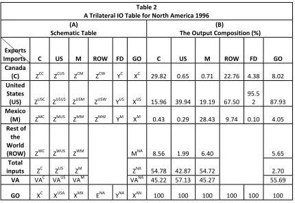
Table 2A illustrates the resulting data ensemble. Going through the columns, one finds the internal transactions matrix (Z) for each country (C, US, and M, respectively), together with the intermediate imports made by each country from each of its partners and from the rest of the world. Adding over the columns, a total input table can be defined as well (domestic plus imported inputs). Further down, there appears a value added matrix (including three rows: compensation to employees, gross operating surplus and net taxes on production; and 32 columns: all the industries considered). Summing up the total inputs and the value added, a gross output value (GO) is thus solved. In an analogous fashion, an internal transactions table appears for each country on each row, showing the intermediate domestic sales to each industry. The other four matrices show exports by sector and country of origin (within North America and the rest of the world). These export matrices are, of course, the imports arrays found on each row: it is assumed that imports for the demanding industry equal exports for the supplier abroad. A final demand matrix is also determined, which is disaggregated by final demand source (household final consumption, non-profit institutions serving households, general government final consumption and gross fixed capital formation) and the 32 sectors. On the Rest of the World column, domestic transactions and value added accounts are missing; the sum across the column corresponds to exports from each country to the rest of the world. Similarly, the final demand account is absent from the row corresponding to this area. The sums across the rows are the total imported inputs from various countries and the rest of the world to each North American country. Matrix ZNA

15 Table 2

A Trilateral IO Table for North America 1996 (A)

Schematic Table

(B)

The Output Composition (%)

Exports

Imports C US M ROW FD GO C US M ROW FD GO

Canada

(C) ZCC ZCUS ZCM ZCW YC XC 29.82 0.65 0.71 22.76 4.38 8.02

United States

(US) ZUSC ZUSUS ZUSM ZUSW YUS XUS 15.96 39.94 19.19 67.50 95.5

2 87.93

Mexico

(M) ZMC ZMUS ZMM ZMW YM XM 0.43 0.29 28.43 9.74 0.10 4.05

Rest of the World

(ROW) ZWC ZWUS ZWM

MNA 8.56 1.99 6.40

5.65 Total

inputs ZC ZUS ZM ZNA 54.78 42.87 54.72 2.70

VA VAC VAUS VAM VANA 45.22 57.13 45.27 55.69

GO XC XUSA XMX ENA YNA XAN 100 100 100 100 100 100

16

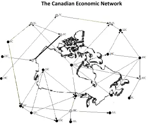
Concerning the disaggregated IO table, 292 ICs were found in the IO table for the North American area; 253 of these (i.e. 3.16% of the total 9216 entries) are located in the three domestic matrices, while 39 ICs are placed in intermediate trade matrices within North America. Therefore, no ICs correspond to intermediate imports from the rest of the world: those links are accessory to the regional relationships in terms of the composition of the productive structure. As a result of the distribution of ICs, Figures 1, 2 and 3 show the internal network of input exchange for each country; each arrow corresponds to a flow of input demand and a thick double-pointed connection corresponds to a reciprocal relationship between two industries.

Figure 1

17 Figure 2

The US Economic Network

Figure 3

18 Sectors

1 AGRICULTURE, HUNTING, FORESTRY AND FISHING

17 RADIO, TELEVISION AND COMMUNICATION EQUIPMENT

2 MINING AND QUARRYING 18 MANUFACTURING NEC AND MEDICAL INSTRUMENTS

3 FOOD PRODUCTS, BEVERAGES AND TOBACCO 19 MOTOR VEHICULES,SHIPS AND BOATS, AIRCRAFT AND SPACECRAFT; AND ROAILROAD EQUIPMENT 4 TEXTILES, TEXTILE PRODUCTS, LEATHER AND

FOOTWEAR

20 ELECTRICITY, GAS AND WATER SUPPLY

5 WOOD AND PRODUCTS OF WOOD AND CORK 21 CONSTRUCTION

6 PULP, PAPER, PAPER PRODUCTS, PRINTING AND PUBLISHING

22 WHOLESALE AND RETAIL TRADE; REPAIRS

7 COKE, REFINED PETROLEUM PRODUCTS AND NUCLEAR FUEL

23 HOTELS AND RESTAURANTS

8 CHEMICALS EXCLUDING PHARMACEUTICALS 24 TRANSPORT AND STORAGE

9 PHARMACEUTICALS 25 POST AND TELECOMMUNICATIONS

10 RUBBER AND PLASTICS PRODUCTS 26 FINANCE, INSURANCE

11 OTHER NON-METALLIC MINERAL PRODUCTS 27 REAL ESTATE ACTIVITIES

12 IRON & STEEL 28 RENTING, MACHINARY ,COMPUTER, RESEARCH, PUBLIC ADMINISTRATION PUBLIC AND PRIVATE HOUSEHOLDS

13 NON-FERROUS METALS 29 OTHER BUSINESS ACTIVITIES

14 FABRICATED METAL PRODUCTS, EXCEPT MACHINARY AND EQUIPMENT

30 EDUCATION

15 MACHINERY AND EQUIPMENT, N.E.C. 31 HEALTH AND SOCIAL WORK

16 OFFICE AND ELECTRICAL MACHINARY 32 OTHER COMMUNITY, SOCIAL AND PERSONAL SERVICES

At first glance, it is clear that the largest proportion of ICs appears in the US internal IO table, which is also the economy that connects the whole economic area and it is known to be, by far, a more developed economy. The US chart shows one hundred and thirty eight (138) arcs; the Canadian one contains fifty four (54); and the Mexican one includes sixty one (61) arcs. The Canadian graph shows nine disconnected sectors; the Mexican one just two; and the US shows no disconnected industries. As a result, density accounts for 0.053 in the Canadian graph; 0.134 in the US; and 0.059 in the Mexican one. Surprisingly, the Canadian and Mexican economies show comparable levels of complexity, despite the well-known differences in per capita income and development levels.

19

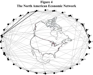
economy is supplemented by its trade partners, which is a consequence of the size gaps existing between them.

Figure 4

The North American Economic Network

Searching for indicators of the way each national structure is built, a feature to be taken into account is whether each of those makes up a solid block or contains a number of isolated or weakly connected subsystems—in the limit, each sector might be disconnected. According to Graph 2, there are seven cut-points in the Canadian network; i.e. if these sectors disappear, they split the graph into eight disconnected subgraphs or components. In the US, there is only one cut-point: sector 21 (construction)3

. It is a sector that demands inputs from branch 11 (other non-metallic products) but, in turn, does not provide inputs to any other industry, so that the demise of sector 11 would isolate sector 21. In Mexico, there are four industries linking other sectors with the core of the system, for which they appear as cut-points in the graph: sector 8 (chemicals, excluding pharmaceuticals), 20 (electricity, gas and water supply), 22 (wholesale, retail and repairs) and 28 (renting machinery, computer research, public administration and public and private households); while sectors 19 (motor

3

20

vehicles, ships and boats, aircraft, spacecraft and railroad equipment) and 29 (other business activities) are the ones isolated in the domestic table. These results account for the complexity of each national graph: the Canadian network is the least integrated, although integration is far from solid in the Mexican one.

21

Table 3

Sectoral Density by Country

Sectors AmericaNorth Canada Estados Unidos Mexico

In Out In Out In Out In Out

1

AGRICULTURE, HUNTING,

FORESTRY AND FISHING 18.8 15.6 6.5 9.7 12.9 12.9 6.5 6.5

2 MINING AND QUARRYING 18.8 6.3 3.2 12.9 12.9 6.5 19.4 3.2

3 FOOD PRODUCTS, BEVERAGES AND TOBACCO 9.4 21.9 6.5 9.7 9.7 22.6 3.2 9.7

4

TEXTILES, TEXTILE PRODUCTS,

LEATHER AND FOOTWEAR 9.4 9.4 3.2 3.2 9.7 12.9 3.2 6.5

5 WOOD AND PRODUCTS OF WOOD AND CORK 12.5 6.3 6.5 9.7 12.9 6.5 9.7 3.2

6 PULP, PAPER, PAPER PRODUCTS, PRINTING AND PUBLISHING 21.9 21.9 9.7 3.2 22.6 16.1 6.5 3.2

7

COKE, REFINED PETROLEUM

PRODUCTS AND NUCLEAR FUEL 15.6 6.3 6.5 6.5 12.9 6.5 9.7 6.5

8

CHEMICALS EXCLUDING

PHARMACEUTICALS 21.9 18.8 3.2 6.5 22.6 19.4 9.7 6.5

9 PHARMACEUTICALS 6.3 6.3 0.0 0.0 6.5 6.5 3.2 0.0

10 RUBBER AND PLASTICS PRODUCTS 31.3 6.3 6.5 9.7 32.3 6.5 12.9 3.2

11 OTHER NON-METALLIC MINERAL PRODUCTS 12.5 3.1 3.2 9.7 6.5 3.2 6.5 3.2

12 IRON & STEEL 18.8 9.4 6.5 9.7 19.4 6.5 9.7 6.5

13 NON-FERROUS METALS 25.0 3.1 0.0 0.0 25.8 3.2 12.9 6.5

14

FABRICATED METAL PRODUCTS, EXCEPT MACHINARY AND

EQUIPMENT 21.9 9.4 6.5 9.7 22.6 12.9 12.9 3.2

15

MACHINERY AND EQUIPMENT,

N.E.C. 9.4 21.9 3.2 3.2 9.7 22.6 3.2 0.0

16 OFFICE AND ELECTRICAL MACHINARY 3.1 15.6 0.0 0.0 3.2 19.4 3.2 3.2

17 RADIO, TELEVISION AND COMMUNICATION EQUIPMENT 9.4 18.8 3.2 3.2 6.5 16.1 3.2 12.9

18

MANUFACTURING NEC AND

MEDICAL INSTRUMENTS 12.5 28.1 0.0 0.0 9.7 29.0 6.5 12.9

19

MOTOR VEHICULES,SHIPS AND BOATS, AIRCRAFT AND

SPACECRAFT; AND ROAILROAD

EQUIPMENT 3.1 34.4 19.4 3.2 3.2 32.3 3.2 3.2

20 ELECTRICITY, GAS AND WATER SUPPLY 6.3 9.4 0.0 12.9 6.5 6.5 0.0 22.6

21 CONSTRUCTION 0 40.6 19.4 0.0 0.0 38.7 6.5 6.5

22 WHOLESALE AND RETAIL TRADE; REPAIRS 3.1 28.1 12.9 0.0 3.2 29.0 0.0 16.1

23 HOTELS AND RESTAURANTS 53.1 12.5 3.2 0.0 61.3 9.7 0.0 6.5

24 TRANSPORT AND STORAGE 0 12.5 6.5 3.2 0.0 12.9 0.0 12.9

25 POST AND TELECOMMUNICATIONS 12.5 12.5 3.2 12.9 12.9 9.7 6.5 0.0

26 FINANCE, INSURANCE 9.4 15.6 12.9 6.5 6.5 12.9 9.7 6.5

27 REAL ESTATE ACTIVITIES 6.3 15.6 0.0 0.0 6.5 16.1 0.0 6.5

28

RENTING, MACHINARY

,COMPUTER, RESEARCH, PUBLIC ADMINISTRATION PUBLIC AND

PRIVATE HOUSEHOLDS 6.3 6.3 16.1 0.0 6.5 6.5 16.1 9.7

29 OTHER BUSINESS ACTIVITIES 6.3 9.4 3.2 19.4 3.2 12.9 0.0 0.0

30 EDUCATION 68.8 3.1 0.0 0.0 77.4 3.2 0.0 3.2

31 HEALTH AND SOCIAL WORK 0 18.8 0.0 3.2 0.0 19.4 9.7 3.2

32

OTHER COMMUNITY, SOCIAL AND

22

In the US, sectors 10 (rubber and plastic products), 13 (non-ferrous metals), 23 (hotels and restaurants) and 30 (education) show the largest amount of incident arcs; they are input providers to the rest of the economy. Their production, however, is below the average output by sector. Perhaps, this is linked to the fact that the US has become an input importer and the impulses from the rest of the system to input producers are not fully transmitted to these relatively smaller activities. On the other hand, sectors with higher density by outdegree are: 3 (food products, beverages and tobacco), 18 (manufacturing N.E.C and medical instruments), 19 (motor vehicles, ships and boats, aircraft, spacecraft and railroad equipment), 21 (construction) and 22 (wholesale, retail and repairs). Sectors 3, 19, 21 and 22 are also among the sectors with above-average contribution to gross output. It is worth highlighting that sectors transmitting influence through intermediate demand seem to be more functional to the dynamics of the economy.

23

4. Trade Patterns in North America

According to results above, international trade represents a smaller proportion of economic transactions for each country, if compared to domestic exchanges; the US being the most autarchic country in the bloc. Figure 5 shows the graph of the IC resulting from the six tables of imports and exports within North America. First, as it has been said above, there are thirty-nine connections only. Second, there is one direct link from the Canadian to the Mexican industries, connecting sectors 19 (motor vehicles, ships and boats, aircraft, spacecraft and railroad equipment) in each of these countries. This sector, however, happens to be dominated by US automobile firms located in both countries and producing massive intrafirm trade, although Canada is also an important producer of railroad equipment, which Mexico is keen to import. On the contrary, sector 19 in Mexico is disconnected from the rest of the domestic economy. Indeed, this is mainly an international sector located within the Mexican territory.

24

Figure 5

The North American Trade Patterns

Sectors

1 AGRICULTURE, HUNTING, FORESTRY AND FISHING

17 RADIO, TELEVISION AND COMMUNICATION EQUIPMENT

2 MINING AND QUARRYING 18 MANUFACTURING NEC AND MEDICAL INSTRUMENTS

3 FOOD PRODUCTS, BEVERAGES AND TOBACCO 19 MOTOR VEHICULES,SHIPS AND BOATS, AIRCRAFT AND SPACECRAFT; AND ROAILROAD EQUIPMENT 4 TEXTILES, TEXTILE PRODUCTS, LEATHER AND

FOOTWEAR

20 ELECTRICITY, GAS AND WATER SUPPLY

5 WOOD AND PRODUCTS OF WOOD AND CORK 21 CONSTRUCTION

6 PULP, PAPER, PAPER PRODUCTS, PRINTING AND PUBLISHING

22 WHOLESALE AND RETAIL TRADE; REPAIRS

7 COKE, REFINED PETROLEUM PRODUCTS AND NUCLEAR FUEL

23 HOTELS AND RESTAURANTS

8 CHEMICALS EXCLUDING PHARMACEUTICALS 24 TRANSPORT AND STORAGE

9 PHARMACEUTICALS 25 POST AND TELECOMMUNICATIONS

10 RUBBER AND PLASTICS PRODUCTS 26 FINANCE, INSURANCE

11 OTHER NON-METALLIC MINERAL PRODUCTS 27 REAL ESTATE ACTIVITIES

12 IRON & STEEL 28 RENTING, MACHINARY ,COMPUTER, RESEARCH, PUBLIC ADMINISTRATION PUBLIC AND PRIVATE HOUSEHOLDS

13 NON-FERROUS METALS 29 OTHER BUSINESS ACTIVITIES

14 FABRICATED METAL PRODUCTS, EXCEPT MACHINARY AND EQUIPMENT

30 EDUCATION

15 MACHINERY AND EQUIPMENT, N.E.C. 31 HEALTH AND SOCIAL WORK

25

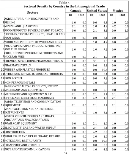
Table 4 contains the density indicators by sector of the above graph. The indegree (In) shows the relative amount of incident arcs to an industry, that is, the number of demanding relations a sector actually maintains as a proportion of the total possible incident arcs. Through this indicator of regional trade, a sector receives influence from producers located abroad, thus inducing it to export goods. In this sense, sectors with higher indegrees in a given economy benefit from some competitive advantage; so, other sectors would seek them as input suppliers. The outdegree (Out) would then show the number of arcs stemming from a sector to the rest of the system: through this indicator, a sector transmits influence by demanding goods from producers abroad. Sectors with higher outdegrees link industries within the system.

The Canadian sectors with higher indegrees in the international North American network are: 2 (mining and quarrying), 5 (wood and products of wood and cork), 15 (machinery and equipment n.e.c.), 17 (radio, television and communication equipment) and 18 (manufacturing n.e.c. and medical instruments). No sector shows a significant outdegree density: industries do not transmit influence (through imports) to their input suppliers located abroad. Canada appears to be a fairly specialised economy, which is able to supply a defined profile of goods to consumers abroad.

In the US, sectors showing higher density by indegree are: 8 (chemicals excluding pharmaceuticals), 16 (office and electrical machinery) and 21 (construction). These receive influence from abroad and export products. Therefore, the whole structure takes advantage of the structural connections of these sectors. On the contrary, sectors transmitting influence through intermediate imports and showing higher outdegrees are: 10 (rubber and plastic products), 13 (nonferrous metals), 23 (hotels and restaurants) and 30 (education).

26

specialised in any specific area of production. This is quite significant, taking into account that Mexico has adopted an export-led growth strategy, but such decision has not been accompanied with the construction of an integrated productive structure. Hence, to a large extent, the country exports goods assembling imported inputs.

Table 4

Sectoral Density by Country in the Intraregional Trade

Sectors Canada United States Mexico

In Out In Out In Out

1AGRICULTURE, HUNTING, FORESTRY AND FISHING 1.0 0.0 0.0 6.3 1.0 0.0

2MINING AND QUARRYING 2.1 0.0 1.0 4.2 4.2 0.0

3FOOD PRODUCTS, BEVERAGES AND TOBACCO 0.0 1.0 2.1 3.1 0.0 1.0

4TEXTILES, TEXTILE PRODUCTS, LEATHER AND FOOTWEAR 0.0 0.0 0.0 3.1 0.0 0.0

5WOOD AND PRODUCTS OF WOOD AND CORK 2.1 0.0 1.0 4.2 0.0 0.0

6PULP, PAPER, PAPER PRODUCTS, PRINTING AND PUBLISHING 1.0 0.0 1.0 7.3 0.0 0.0

7COKE, REFINED PETROLEUM PRODUCTS AND NUCLEAR FUEL 0.0 0.0 2.1 4.2 0.0 0.0

8CHEMICALS EXCLUDING PHARMACEUTICALS 1.0 0.0 3.1 7.3 1.0 0.0

9PHARMACEUTICALS 0.0 0.0 0.0 2.1 0.0 0.0

10RUBBER AND PLASTICS PRODUCTS 0.0 0.0 0.0 10.4 0.0 0.0

11OTHER NON-METALLIC MINERAL PRODUCTS 1.0 0.0 0.0 2.1 0.0 0.0

12IRON & STEEL 0.0 1.0 0.0 7.3 0.0 0.0

13NON-FERROUS METALS 0.0 0.0 1.0 8.3 1.0 0.0

14FABRICATED METAL PRODUCTS, EXCEPT MACHINARY AND EQUIPMENT 0.0 0.0 0.0 7.3 0.0 0.0

15MACHINERY AND EQUIPMENT, N.E.C. 2.1 0.0 2.1 3.1 3.1 0.0

16OFFICE AND ELECTRICAL MACHINARY 1.0 0.0 4.2 1.0 2.1 0.0

17RADIO, TELEVISION AND COMMUNICATION EQUIPMENT 2.1 0.0 2.1 2.1 2.1 0.0

18MANUFACTURING NEC AND MEDICAL INSTRUMENTS 7.3 0.0 1.0 3.1 1.0 0.0

19

MOTOR VEHICULES,SHIPS AND BOATS, AIRCRAFT AND SPACECRAFT; AND

ROAILROAD EQUIPMENT 0.0 1.0 2.1 1.0 1.0 0.0

20ELECTRICITY, GAS AND WATER SUPPLY 0.0 0.0 2.1 2.1 0.0 0.0

21CONSTRUCTION 0.0 0.0 4.2 0.0 0.0 0.0

22WHOLESALE AND RETAIL TRADE; REPAIRS 0.0 0.0 1.0 1.0 0.0 0.0

23HOTELS AND RESTAURANTS 0.0 0.0 0.0 19.8 0.0 0.0

24TRANSPORT AND STORAGE 0.0 0.0 0.0 0.0 0.0 0.0

27

26FINANCE, INSURANCE 0.0 0.0 0.0 2.1 0.0 0.0

27REAL ESTATE ACTIVITIES 0.0 0.0 0.0 2.1 0.0 0.0

28

RENTING, MACHINARY ,COMPUTER,

RESEARCH, PUBLIC ADMINISTRATION PUBLIC

AND PRIVATE HOUSEHOLDS 0.0 0.0 5.2 2.1 0.0 0.0

29OTHER BUSINESS ACTIVITIES 0.0 0.0 0.0 1.0 0.0 0.0

30EDUCATION 0.0 0.0 0.0 25.0 0.0 0.0

31HEALTH AND SOCIAL WORK 0.0 0.0 0.0 0.0 0.0 0.0

32OTHER COMMUNITY, SOCIAL AND PERSONAL SERVICES 0.0 0.0 0.0 0.0 0.0 0.0

Conclusions

In this paper we have found a North American economic network that shows the structural connections existing between sectors in Canada, the US and Mexico. Analysing that structure we conclude that the three economies are highly interdependent, because in each country intermediate imports from other North American countries are essential to carry out production in various industries. Nevertheless, sectors within each economy are primarily linked to domestic sectors, secondly to branches within North America and thirdly to industries beyond. In that sense, the North American network contains three interconnected subsystems, one for each country.

The complexity of an economic system has been defined as the amount of connections between industries relative to the maximum possible amount of interindustry liaisons. In North America, the US is the most complex subsystem; it is also less dependent upon imports from its neighbouring partners, but keeps closer trade relationships with the rest of the World. Canada and Mexico maintain scarce direct relationships and import intermediate goods mainly from the U.S. The complexity of their subsystems is also lower. Influence will expand more easily through a complex network, because industries will be connected through a larger amount of paths, involving more sectors. This paper uses density as an indicator of the complexity of the system.

28

connections -forming the core of the structure- there are also groups of industries connected to that core through one particular sector only (called cutpoint). The Canadian subsystem can easily be split into disconnected groups if the connections if such cutpoints demise; moreover, there are also a few sectors totally disconnected. The Mexican subsystem contains fewer cutpoints, but it shows a level of complexity comparable to that of Canada. Apparently, in both cases integration with North America has encouraged that domestic sectors cultivate connections with US industries, rather than maintaining stronger links to domestic sectors, as has been the case in the US. In Canada the structure is based upon the extractive sectors; in Mexico the manufacturing industry has turned to assemble imported components to export goods; these activities are barely related to the domestic productive sector, for which exports show low multipliers and probably that is one reason for which the economy shows low growth rates. The benefits of constructing a single economic area are not clear for Canada or Mexico.

Lastly, it is both the high and low technology sectors that define the complexity of the economic network in North America. Such a feature is observed also for the US, but that is not obvious for neither Canada or in Mexico, where high technology sectors are smaller and import larger proportions of inputs. Medium technology industries are also more important for these two countries.

29

References

1. Aroche Reyes Fidel ( 1996) “Important Coefficients and Structural Change: A Multi -layer Approach” Economic Systems Research, Vol. 8, No. 3 pp. 235-246

2. Campbell John (1975) “Application of Graph Theoretic Analysis to Interindustry

Relationships, The example of Washington State” Regional Science and Urban Economics Vol. 5, No. 1, pp. 91-106.

3. Carter Anne (1970) Structural Change in the American Economy. Cambridge, Mass.: Harvard University Press

4. Czamanski Stan and Luiz A. Ablas (1979) “Identification of Industrial Clusters and Complexes: A Comparison Methods and Findings” Urban Studies, Vol. 16, No. 1 pp. 62 – 80.

5. Curzio Leonardo (2009). La competitividad en América del Norte y el modelo de integración. México, D.F.: Cuadernos de América del Norte No. 13, Centro de Investigaciones Sobre América del Norte (CISAN), UNAM.

6. Defourny Jacques (1982) “Une approche structurale pour l’analyse Input – Output: un

premier bilan” Economie appliquée Tome XXXV No. 1 – 2 pp. 203 – 230.

7. De Mesnard Louis (1995), “A Note on Qualitative Input-Output Analysis” Economic Systems Research, Vol. 7, No. 4, pp. 439-445

8. De Mesnard Louis (2001) “On Boolean Topological Methods of Structural Analysis”, Lahr, M.L. and Dietzenbacher, E. (eds.): Input-Output Analysis: Frontiers and Extensions, New York: Palgrave, pp. 268-279.

9. Forsell Ösmo (1983) “Experiences of Studying Changes in Input- Output Coefficients in Finland” E Smyshliav, A. (ed.) Proceedings of the Forth IIASA Task Force Meeting on the I – O Model. IIASA collaborative proceedings series. Vienna: National Technical Information Service, distributor.

10. Gould R. (1988) Graph Theory London: The Benjamin/Cummings Publishing Company, Inc.

11. Harary F. (1969) Graph Theory. Reading, Ma.: Addison – Wesley

12. Holub H. W. And Schnabl, H. (1985) Qualitative Input – Ouput Analisys and Structural Information, Economic Modelling, Vol. 20, pp. 173 -195.

13. Huriot Jean M (1974): Dependence et Hiérarchie dans une Structure Interindustrielle Paris: Sirey.

14. Isard Walter (1951) “Interregional and regional input-output analysis: A model of a

space economy” The Review of Economics and Statistics Vol. 33, pp. 318-328.

15. Leontief Wassily (1951) The Structure of American Economy, 1919-1939: An Empirical Application of Equilibrium Analysis. Oxford: Oxford University Press.

16. Miller Ronald E. y Peter D. Blair (2009), Input-Output Analysis: Foundations and Extensions, Cambridge, Cambridge University Press.

17. Schinkte J. and Stänglin R. (1988) “Important Input Coefficients in the Market

Transactions Tables and Production Flow Tables” M Ciaschini (ed.) Input – Output Analysis: Current Developments. London: Chapman and Hall.

30

19. Semitiel García María (2006) Social Capital, Networks and Economic Development: An Analysis of Regional Productive Systems. Cheltenham: Edward Elgar Publishing.

20. Skolka Jiri (1983) “Important Input Coefficients in Austria Input – Output Tables for

1964 and 1976” in Smyshliav, A (ed.) Proceedings of the Forth IIASA Task force

Meeting On The I – O Model, Vienna: National Technical Information Service, Distributor.

21. Wientraub Sydney (2004) “Trade, Investment and Economic Growth” Weintraub S.