Munich Personal RePEc Archive
Parameter Estimation and Model Testing
for Markov Processes via Conditional
Characteristic Functions
Chen, Songxi and Peng, Liang and Yu, Cindy
2013
Parameter Estimation and Model Testing for Markov
Processes via Conditional Characteristic Functions
Song Xi Chena,b, Liang Pengc and Cindy L. Yua
a Department of Statistics, Iowa State University, Ames, Iowa 50011-1210, USA
b Guanghua School of Management and Center for Statistical Science
Peking University, Beijing 100871, China
c School of Mathematics, Georgia Institute of Technology, Atlanta, GA 30332
Abstract: Markov processes are used in a wide range of disciplines including finance.
The transition densities of these processes are often unknown. However, the conditional
characteristic functions are more likely to be available especially for L´evy driven processes.
We propose an empirical likelihood approach for both parameter estimation and model
specification testing based on the conditional characteristic function for processes with
either continuous or dis-continuous sample paths. Theoretical properties of the empirical
likelihood estimator for parameters and a smoothed empirical likelihood ratio test for a
parametric specification of the process are provided. Simulations and empirical case study
are carried out to confirm the effectiveness of the proposed estimator and test.
Keyword: Conditional characteristic function; Diffusion processes; Empirical likelihood;
Kernel smoothing; L´evy driven processes
1
Introduction
Let {Xt(θ)}t∈T be a parametric d-dimensional Markov process defined by
where µ(·) is a d-dimensional drift function, σ(·) is a d× d matrix-valued function of
Xt, Lt;θ is a L´evy process in Rd, and θ ∈ Θ ⊂ Rp. When Lt is a standard Brownian
motion, (1.1) is a diffusion process having a continuous sample path. When Lt contains
the Brownian motion and a compound Poisson process, (1.1) becomes the jump diffusion
process. A stochastic process of form (1.1) has long been used to model stochastic systems
arising in physics, biology and other natural sciences. It has also been the fundamental
tool in financial modeling. We refer to Sundaresan (2000) and Fan (2005) for overviews,
Barndorff-Nielsen, Mikosch and Resnick (2001) for recent developments on L´evy driven
processes, and Sørensen (1991) for statistical inference. Important subclasses of (1.1)
include i) the multivariate diffusion process defined by
dXt=µ(Xt;θ)dt+σ(Xt;θ)dBt, (1.2)
where Bt is the standard Brownian motion in Rd (Stroock and Varadhan, 1979 and
Øksendal, 2000); ii) the Vasicek with Merton Jump model (VSK-MJ) defined by
dXt=κ(α−Xt)dt+σdBt+JtdNt, (1.3)
where κ, α and σ are unknown parameters and represent the mean reverting rate,
long-run mean and volatility of the process respectively, Nt is a Poisson process with intensity
λ, and Jt is the random jump size independent of the filtrationFt up to time t and has
a normal density N(0, η2) (Merton, 1976); iii) L´evy driven Ornstein-Uhlenbeck process
defined by
dXt=−λXtdt+dLλt, X0 >0, (1.4)
where Lt is a L´evy process with no Brownian part, a non-negative drift and a L´evy
measure which is zero on the negative half line, and the parameter λ is positive (see
Barndorff-Nielsen and Shephard, 2001).
Often a closed form expression for the transition density of process (1.1) is not available
fact prevents the use of the maximum likelihood estimation (MLE) and the specification
tests based on the exact transition density. Recently A¨ıt-Sahalia(2002, 2008) established
expansions for the transition densities so that parameter estimation can be based on the
approximate likelihood functions. Testing may be also formulated via the approximate
density; see Chen, Gao and Tang (2008) and A¨ıt-Sahalia, Fan and Peng (2009) for such
tests. The conditional characteristic functions (CCF) are more likely available than the
transition densities for the continuous-time models, especially for the L´evy driven
pro-cesses through the celebrated L´evy-Khintchine representation. For instance, Duffie, Pan
and Singleton (2000) derived the explicit form of the CCF for multivariate affine jump
processes, which include the Vasicek with Merton jump process given in (1.3). The CCF
for the L´evy driven Ornstein-Uhlenbeck process (1.4) is established in Barndorff-Nielsen
and Shephard (2001).
Statistical inference based on the characteristic functions was proposed by Feuerverger
and Mureika (1977), Feuerverger and McDunnough (1981) for independent observations
and Feuerverger (1990) for discrete time series. Singleton (2001) introduced the approach
to inference for parametric continuous-time Markov processes and show that estimation
can be carried out based on the CCF without having to carry out the the Fourier inversion.
Chacko and Viceira (2003) proposed a generalized method of moment estimator (GMM)
for parameters at a finite number of frequencies of the CCF. Carrasco, Chernov, Florens
and Ghysels (2007) carried out GMM estimation on a slowly diverging number of
frequen-cies of the CCF to achieve the optimal estimation efficiency offered by the MLE. Jiang
and Knight (2002) proposed GMM estimators based on the joint characteristic function
of the observed state variables. Chen and Hong (2010) proposed a test for multivariate
processes based on the CCF via a generalized spectral density approach.
In this paper, we first propose an empirical likelihood (Owen, 1988) approach for
via the CCF. An empirical likelihood ratio is formulated for the unknown parameters
assuming the specification (1.1), which leads to a non-parametric maximum likelihood
estimator. The proposed estimator may be viewed as a compromise between Chacko
and Viceira (2003)’s GMM based on a finite number of frequencies and that of Carrasco,
Chernov, Florens and Ghysels (2007) of a high dimensional GMM. The high dimensional
GMM approach requires ridging a high dimensional weighting matrix in order to avoid
its singularity, and the selecting the ridging parameter can be computationally expensive.
The proposed estimation utilizes a wide range of frequency information in the parametric
CCF, while having the computation easily managed.
We then formulate an empirical likelihood CCF based model specification test for the
parametric process (1.1) via kernel smoothing. The proposed test extends the transition
density based tests of Hong and Li (2005), Chen, Gao and Tang (2008) and A¨ıt-Sahalia,
Fan and Peng (2009) to the CCF based. This largely increases the range of the
continuous-time Markov processes which can be tested directly without replying on the transition
density approximation. The proposed test provides an alternative formulation of the
CCF based test of Chen and Hong (2010), which is based on an explicit L2 measure
between an kernel estimator of the CCF and its parametric counter-part. It is largely
distinct from the above mentioned tests, except Chen and Hong (2010), by targeting
directly on CCF, which is more readily available for continuous-time models than the
transition density functions. Another advantage of the proposed test is the empirical
likelihood (EL) formulation, which can produce an integrated likelihood ratio test in a
nonparametric setting. The proposed test utilizes some of the attractive properties of
the EL, like internal studentizing without an explicit variance estimation and good power
performance. How to extend the proposed methods to the case of latent variables is quite
challenging and will be a part of our future research.
based empirical likelihood estimator. The model specification test is given in Section 3.
Section 4 reports results from simulation studies. An empirical study for a set of 3-month
treasury bill rate data is analyzed in Section 5. All technical details are reported in the
Appendix.
2
Parameter Estimation
Let {Xtδ}nt=1 be n discretely sampled observations of (1.1). For notation simplification,
we denote Xtδ as Xt, where the sampling interval δ is any fixed quantity. Let ψt(u;θ) =
Eθ(eiu
TX t+1|X
t), for u ∈ Rd, be the conditional characteristic function. We use ¯a and
A⋆ to denote the conjugate of a complex number a and the conjugate transpose of the
complex matrix A, respectively.
Letǫt(τ;θ) =w(u, r;Xt){eiu
TX t+1−ψ
t(u;θ)}forτ = (uT, rT)T ∈R2d, wherew(u, r;Xt)
is a weight factor. Here ǫt(τ;θ) can be regarded as ’residuals’ between eiu
TX
t+1 and the
parametric CCF ψt(u;θ). The complex weight factor w(u, r;Xt) satisfies ¯w(u, r;Xt) =
w(−u,−r;Xt) and |w(u, r;Xt)|= 1 for any u, r ∈Rd, whose use is aimed to utilize more
model information. Let θ0 be the true parameter and the unique solution of
E{eiuTXt+1
−ψt(u;θ)|Xt}= 0 for all u∈Rd. (2.1)
From the Markov property and (2.1), for any τ = (uT, rT)T ∈R2d
E{ǫt(τ;θ0)}= 0 and Cov{ǫt1(τ;θ0), ǫt2(τ;θ0)}= 0 if t1 =t2. (2.2)
Let ǫR
t(τ;θ) and ǫIt(τ;θ) be the real and imaginary parts of ǫt(τ;θ) respectively, and
ǫt(τ;θ) =
ǫRt(τ;θ), ǫIt(τ;θ)
T
be the real bivariate vector corresponding to ǫt(τ;θ).
We now formulate an empirical likelihood for θ based on the CCF ψt(u;θ). The
of a non-parametric likelihood for parameters of interest. Despite that the EL method is
intrinsically non-parametric, it possesses two important properties of a parametric
likeli-hood, the Wilks’ theorem and the Bartlett correction; see Chen and Van Keilegom (2009)
for a latest overview and Kitamura, Tripathi and Ahn (2004) for a formulation with
conditional moments.
Letp1(τ),· · ·, pn(τ) be probability weights allocated to the ’residuals’{ǫt(τ;θ)}nt=1. A
local EL for θ atτ is
Ln(τ, θ) = max n
t=1
pt(τ) (2.3)
subject to n
t=1pt(τ) = 1 and nt=1pt(τ)ǫt(τ;θ) = 0. Here the second constraint reflects
(2.1). The maximum empirical likelihood is attained atpt(τ)≡n−1 for all tsuch that the
maximum likelihood Ln(τ;θ) = n−n. Let ℓn(τ;θ) = −2 log{Ln(τ;θ)/n−n} be the local
log-EL ratio of θ atτ.
Employing the EL algorithm (Owen, 1988), the optimalpt(τ) of the above optimization
problem (2.3) is
pt(τ) =
1
n
1 1 +λ(τ;θ)Tǫ
t(τ;θ)
,
where λ(τ;θ) is a Lagrange multiplier in R2 that satisfies
Q1n(τ;θ, λ) =:
1
n
n
t=1
ǫt(τ;θ)
1 +λ(τ;θ)Tǫ t(τ;θ)
= 0. (2.4)
Hence, the local EL ratio becomes
ℓn(τ;θ) = 2 n
t=1
log{1 +λ(τ;θ)Tǫt(τ;θ)}. (2.5)
Integrating ℓn(τ;θ) against a probability weight π(τ) which is supported on a compact
set S in R2d, an integrated empirical likelihood ratio forθ is
ℓn(θ) =
τ∈R2dℓn(τ;θ)π(τ)dτ. (2.6)
The maximum EL estimator (MELE) for θ is defined as
ˆ
by noting that −2 has been multiplied in the EL ratio ℓn(τ;θ).
Like Qin and Lawless (1994), we first show that there exists a consistent estimator ˆθn
with a certain rate of convergence as follows.
Lemma 1. Under conditions C1-C4 given in the appendix, with probability one, ℓn(θ)
attains its minimum at ˆθn in the interior of the ball ||θ −θ0|| ≤ O(n−1/3), and ˆθn and
λ(τ; ˆθn) satisfy
Q1n(τ; ˆθn, λ(τ; ˆθn)) = 0 for all τ ∈S and
Q2n(τ; ˆθn, λ(τ; ˆθn))π(τ)dτ = 0,
(2.7)
where Q1n is defined in (2.4) and
Q2n(τ;θ, λ) =
1 n n t=1 1 1 +λ(τ;θ)Tǫ
t(τ;θ)
∂ǫT t (τ;θ)
∂θ λ. (2.8)
Before deriving the asymptotic normality of the ˆθn, we define
M0 = 12
1 1
i−1 −i−1
, ˜ǫt(τ;θ) = (ǫt(τ;θ), ǫt(−τ;θ))T,
A(τ1, τ2;θ0, θ) = Cov{˜ǫ1(τ1;θ),˜ǫ1(τ2;θ)},
Γ(θ0) =:
E
∂˜ǫ⋆ 1(τ;θ0)
∂θ
A−1(τ, τ;θ0, θ0)E
∂˜ǫ1(τ;θ0)
∂θ
π(τ)dτ, (2.9)
and
V(θ0) = E
∂˜ǫ⋆
1(τ1;θ0)
∂θ
A−1(τ
1, τ1;θ0, θ0)A(τ1, τ2;θ0, θ0)
×A⋆−1(τ
2, τ2;θ0, θ0)E
∂˜ǫ
1(τ2;θ0)
∂θ
π(τ1)π(τ2)dτ1dτ2.
(2.10)
Theorem 1: Under Conditions C1-C4 given in the appendix, for the estimator ˆθn in
Lemma 1, we have √n(ˆθn−θ0)→d N(0,Σ) where Σ = Γ−1(θ0)V(θ0)Γ−1(θ0).
The proposed estimator attains the√n-rate of convergence. It is computationally sta-ble because computingℓn(τ;θ) for oneτ at a time is essentially one dimensional problem.
Note that Carrasco, Chernov, Florens and Ghysels (2007) considered CCF based
space via covariance operator, but the covariance operator may not be invertible due to
zero eigenvalues. Hence, Carrasco, Cherno, Florens and Ghysels (2007) needed ridging
to avoid the invertible issue, which makes the computation quite involved. When the
dimension of θ is not small, it would be useful to replace the equation n
t=1ptǫt(τ;θ) = 0
in formulating the local EL in (2.3) by several equations such as
n
t=1
ptǫt(s1τ;θ) = 0,· · ·, n
t=1
ptǫt(smτ;θ) = 0
for some given s1,· · ·, sm.
3
Test for Model Specification
In this section we consider testing for the validity of (1.1) via testing for the parametric
specification of the CCF ψt(u;θ). Tests for model specification of a continuous-time
Markov process have been proposed by Chen, Gao and Tang (2008) and A¨ıt-Sahalia,
Fan and Peng (2009). Despite parameter estimation based on the transition density is
asymptotically efficient, it is unclear if a test based on the transition density is more
powerful than one based on the CCF. The choice is clearer when the transition density
does not admit a closed form while the CCF does, since the latter is a test valid at any
level of the sampling interval δ.
Let the underlying process that generates the observed sample path {Xt}nt=1 be
dXt =µ(Xt)dt+σ(Xt)dLt, (3.1)
whose CCF is ψ(u;Xt). The process (1.1) is a parametric specification of (3.1). To
emphasize the dependence of the CCF on Xt, we write in this section ψt(u) asψ(u, Xt),
ψt(u;θ) as ψ(u, Xt;θ) and other quantities in a similar fashion. We consider testing
against a sequence of local alternative hypotheses
H1 :P{ψt(u) =ψt(u;θ0) +cn∆n(u;Xt)}= 1 for all u∈Rd,
where {cn} is a sequence of non-random real constants converging to zero at a certain
rate, and {∆n(u;Xt)} is a sequence of bounded complex functions which are continuous
at u= 0 and ∆n(0;Xt)≡0; see Condition C6 in the appendix for extra restrictions.
Since the target of inference is a conditional quantity, we need to work with a kernel
smoothed version of ℓn(θ). Let K be a kernel function which is a symmetric probability
density in Rd, and h be a smoothing bandwidth that tends to 0 as n → ∞. A smoothed
version of Ln(τ, θ) is
Lnh(τ, x;θ) = max n
t=1
pt(τ, x) (3.2)
subject to n
t=1pt(τ, x) = 1 and nt=1pt(τ, x)Kh(x−Xt)ǫ(τ, Xt;θ) = 0.
Let ℓnh(τ, x, θ) = −2 log{Lnh(τ, x, θ)nn} be the log-EL ratio. Then, the integrated
log-EL ratio for θ is
ℓnh(θ) =
ℓnh(τ, x, θ)π1(τ)π2(x)dτ dx
where π1 and π2 are probability weight functions on the frequency space and the state
space respectively. We can choose π1 to be the same as the π in Section 3.
The test statistic is ℓnh(ˆθn), where ˆθnis the empirical likelihood estimator proposed in
Section 3. As a matter of fact, we can employ any estimator withn1/2-rate of convergence.
To appreciate the meaning of the test statistic, letWh(x−Xt) =Kh(x−Xt)/nj=1Kh(x−
Xj) be the Nadaraya-Watson kernel weight, ǫn,h(τ, x;θ) = nt=1Kh(x−Xt)ǫ(τ, Xt;θ) be
the kernel smooth of the residuals,
˜
ǫn,h(τ, x;θ) = (ǫnh(τ, x;θ), ǫnh(−τ, x;θ))T, and R(K) = K2(t)dt. It can be shown by a
similar derivation in Chen, H¨ardle and Li (2003) that
ℓnh(θ) = nhdR−1(K) ˜ǫ⋆n,h(τ, x;θ)V−1(τ, x;θ0, θ)˜ǫn,h(τ, x;θ)
×π1(τ)f(x)π2(x)dτ dx+Op{(nhd)−1/2log3(n) +h2log2(n)},
where V(τ, x;θ0, θ) =V ar{ǫ˜(τ, Xt;θ)|Xt=x} and f(x) is the density of Xt. So, the test
statistic is asymptotic equivalent to a L2-measure of the averaged ’residuals’ ˜ǫ⋆n,h(τ, x;θ)
inversely weighted by the covariance matrix function V. Hence, the proposed test is
similar in tune to Fan and Zhang (2003) for testing diffusion processes, and of H¨ardle and
Mammen (1993) and Wang and Van Keilegom (2007) for testing regression functions.
We need the following notations to describe the power property. Let V(τ1, τ2, x) =
E{˜ǫ(τ1, Xt;θ0)˜ǫ⋆(τ2, Xt;θ0)|Xt = x}, then V(τ, τ, x;θ0, θ0) = V(τ, x) defined earlier.
Ex-press the matrices
V(τ1, τ2, x) = (Vlk(τ1, τ2, x))1≤l,k≤2 and V
−1(τ, x) =
νlk(τ, x)
1≤l,k≤2.
Furthermore, we choose cn=n−1/2hd/4 and define
ηn(τ, Xt) =w(τ;Xt)∆n(u, Xt), η˜n(τ, Xt) = (ηn(τ, Xt), ηn(−τ, Xt))T,
µn=
˜
ηn⋆(τ, x)V−1(τ, x;θ0, θ0)˜ηn(τ, x)π1(τ)π2(x)f(x)dτ dx,
σ2
n = 2R−2(K)h−dγ2(K, V, π1, π2) where
γ2(K, V, π1, π2) = K(4)(0)
2
l1,k1,l2,k2
Vl1l2(−τ1, τ2, x)Vk1k2(τ1,−τ2, x)ν
l1,k1
(τ1, x)
× νl2,k2(τ
2, x)π1(τ1)π1(τ2)π22(x)dτ1dτ2dx. (3.4)
where K(4) is the 4-th convolution of the kernel function K.
The asymptotic normality of ℓnh(ˆθn) is given in the following theorem.
Theorem 2Under Conditions C1-C6 given in the appendix,
h−d/2(ℓ
nh(ˆθn)−2−hd/2µn)→d N(0,2R−2(K)γ2(K, V, π1, π2)). (3.5)
We note thatµn= 2 underH0. UnderH1, since ∆n(u, x) is non-vanishing with respect
tou, ˜ηn(τ, x) is non-vanishing with respect to ufor all xin the support of f, which leads
restriction has been imposed on the functional form of ∆n(u, Xt), it means that the test
is powerful for a wide range of local alternatives. Indeed, if ˆγ2(K, V, π
1, π2) is a consistent
estimator of γ2(K, V, π1, π2), the asymptotic normality based test for H0 with α-level of
significance rejects H0 if
ℓnh(ˆθn)≥2 +z1−α
√
2hd/2R−1(K)ˆγ(K, V, π1, π2),
where z1−α is the 1−α quantile of the standard normal distribution. Theorem 2 implies
that the power of the test under H1 is
Φ
−z1−α+
R(K)µn
√
2γ(K, V, π1, π2)
,
where Φ is the standard normal distribution function.
It is known that the choice of bandwidth is important in any test based on the kernel
smoothing technique. To make the test less sensitive to the choice of smoothing
band-width, we propose carrying out the test based on a set of bandwidths, say {h1,· · ·, hk},
for a fixed integer k such that hi =cih for some constantsc1 < c2 < ... < ck. Here h is a
reference bandwidth which may be obtained via the cross-validation method.
This means that we have a set of the EL ratios {ℓnh1(ˆθn),· · ·, ℓnhk(ˆθn)} corresponding
to the bandwidth set, and the overall test statistic is
Tn= max 1≤i≤k{h
−d/2
i (ℓnhi(ˆθn)−2)}. (3.6)
To describe the asymptotic distribution of Tn, let K(2)(z, c) = K(u)K(z+cu)du be
a generalization to the convolution of K, ν(t) = {K(2)(tu, t)}2
du and
ΣJ =
2
R2(K)
π1(τ1)π1(τ2)π22(x)dxdτ1dτ2
(cj/ci)dν(ci/cj)
J×J.
Theorem 3. Under Conditions C1-C6, Tn →d max1≤k≤JZk as n→ ∞ where
Lettα be the 1−α quantile ofTn whereα ∈(0,1) is the nominal size of the test. The
following parametric bootstrap procedure is employed to approximate tα:
Step 1: Simulate a sample path {X∗
t}nt=1 at the same frequency δ according to the
model under H0 with the CCF based estimate ˆθn.
Step 2: Let ˜θ∗
nbe the estimate ofθunderH0 using the resample path{Xt∗}nt=1obtained
in Step 1, and T∗
n be the version of Tn for the resampled path.
Step 3: For a large positive integer B, repeat Steps 1 and 2 B times and obtain, after
ranking, T(1)∗
n ≤Tn(2)∗ ≤ · · · ≤Tn(B)∗.
Then, the Monte Carlo approximation of tα isTn([B(1−α)]+1)∗. The proposed test rejects
H0 if Tn(ˆθn) ≥ Tn([B(1−α)]+1)∗. The justification of the above bootstrap procedure can be
made based on Theorem 3 via the standard techniques for instance those given in Chen,
Gao and Tang (2008).
4
Simulation Study
We report in this section the results from our simulation studies which are designed to
verify the proposed parameter estimator and model testing procedure. To evaluate the
quality of the proposed EL estimator, we first chose two univariate diffusion processes
with known transition densities, so that the MLEs can be compared with the proposed
EL estimates. The two processes are the Vasicek model (Vasicek, 1977) (VSK),
dXt=κ(α−Xt)dt+σdBt, (4.1)
and the Cox-Ingersoll-Ross Model (Cox, Ingersoll and Ross, 1985) (CIR),
dXt=κ(α−Xt)dt+σ
XtdBt, (4.2)
whereκ,α andσ are unknown parameters which represent the mean reverting rate,
interest rate modeling and various option price formulation. For the Vasicek model, the
transition distribution ofXt+1|Xtis a normal distributionN(α+(Xt−α)exp(−κδ), σ2(1−
exp(−2κδ))/(2κ)). For the CIR model, when 2κα/σ2 >1,Xt+1|Xtis a multiple of a
non-central Chi-square random variable with degrees of freedom 4κα/σ2 and non-centrality
parametercXtexp(−κδ), where the multiplier is 1/cwithc= 4κ/(σ2(1−exp(−κδ))). The
CCFs of these two models can easily be derived from their known transitional densities.
We then considered estimation for the jump diffusion model VSK-MJ as given in (1.3)
based on its CCF function
ψt(u;θ) = exp{
σ2u2
4κ (e
−2κδ
−1)−λδ+γ+i(αu(1−e−κδ) +ue−κδX
t)}, (4.3)
where γ =λ/(2κ) e1−2κδexp(−η
2u2y/2)/ydy. For comparison, we approximated its
tran-sition density by a mixture of normal distributions, (1−λδ)N(µδ, σ2δ) +λδN(µδ, σδ2+η2),
which is a first order approximation proposed in A¨ıt-Sahalia, Fan and Peng (2009). Here,
µδ =α+ (Xt−α)exp(−κδ), and σδ2 =σ2(1−exp(−2κδ))/(2κ). The approximate MLEs
were obtained based on the mixture approximation given above.
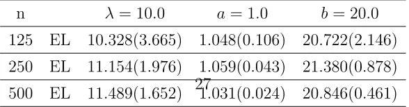
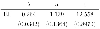
We also consider the Inverse Gaussian OU process (IG-OU) in (1.4), i.e. the processXt
follows the Inverse Gaussian lawIG(a, b), for every twhen X0 is generated fromIG(a, b).
The CCF of this process is
ψt(u;θ) =exp{−a(
√
−2iu+b2−−2iue−λδ+b2) +iue−λδX
t}. (4.4)
Since neither the exact transition density nor its approximation is available, we were
content with carrying out estimation with the proposed methods.
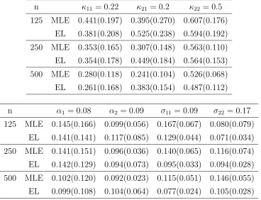
The last simulation model considered for the estimation is a bivariate extension of the
univariate Ornstein-Uhlenbeck process (BI-OU),
dXt=κ(α−Xt)dt+σdBt, (4.5)
where Xt = (X1t, X2t), κ =
κ11 0
κ21 κ22
, α =
α1
α2
and σ =
σ11 0
0 σ22
. Under
stationary with transition distribution being a bivariate normal N(m(δ, Xt),Ω(δ)) where
m(δ, Xt) =α+exp(−κδ)(Xt−α), Ω(δ) = Σ−exp(−κδ)Σexp(−κTδ) and
Σ = 1
2tr(κ)Det(κ){Det(κ)σσ
T +
{κ−tr(κ)}σσT{κ−tr(κ)}T}.
The CCF of the process is known to beψt(u1, u2;θ) =exp{iuTm(δ, Xt)−uTΩ(δ)u/2}for
u= (u1, u2)T.
We then carried out simulations to evaluate the ability of the proposed tests in
detect-ing model deviations. When we chose the simulation models, we had in mind two issues
in finance that have drawn considerable research attention recently. The first issue is
whether the process is subject to jumps, and the second is whether we could differentiate
two processes with different jump rates. Our simulation study formulated two settings of
hypotheses to address these two issues. In the first setting, we tested
H0 : The process is the VSK model.
In the second setting, we tested
H0 : The process is the jump diffusion model VSK-MJ.
For computing the powers, in the first setting we used the data simulated from H1 :
the jump diffusion model VSK-MJ to test the null model which does not have jumps; in
the second setting, we used the data simulated from H1 : the Inverse Gaussian OU model
which has infinite-activity jumps to test the null hypothesis that prescribes a finite-activity
jump process.
For each model, we simulated 500 sample paths which were observed at monthly
observations (δ = 1/12) for n = 125,250,500 respectively. The choices of parameter
values were motivated by Chen, Gao and Tang (2008) and Ait-Sahalia, Fan and Peng
In parameter estimation, we discovered that for both real and imaginary parts of
the CCF, their non-parametric smoothing estimators are wave-like functions and roughly
diminish to zero at the same points, which creates a region denoted as St (here the
subscript tindicates that the region depends onXt). In practice, we searched on a couple
of grid points in the data range of Xt and picked the union ofSt as the support region S
for the frequency domain ofψt(u;θ) in the estimation. We then chose the uniform density
as the weight function π over the support region.
In model testing, similar effort was initially made to obtain the support region of the
non-parametric CCF estimate, denoted as SN P, and the support region of the theoretical
CCF under H0, denoted as SH0. Here the theoretical CCF under H0 used ˆθn from our
EL method. Then the support region of the frequency domain in testing was taken as
the union of SN P and SH0. We chose the uniform density as the weight function over
this support region for testing. There is little contribution to the integrated empirical
likelihood ratio ℓnh(ˆθn) from outside the support region. The biweight Kernel K(u) =
15/16(1−u2)2I(|u| ≤ 1) was used for smoothing in testing. The bandwidth selection is
described in Section 3. The bandwidth sets were specified in Tables 3 and 4 for the two
test settings. It is observed that the values of the bandwidths were quite small, which
was due to the rapid oscillation of the CCF curves which favored smaller bandwidth in
the curve fitting.
We chose w(u, r;Xt) = eir
TX
t throughout our simulation study as it is the optimal
instrument suggested in Carrasco, Chernov, Florens and Ghysels (2007). Some numerical
exploration (not reported) indicated the choice of the function w(·) is not crucial in the context of the paper. For testing, we picked the unit instrument to reduce computing
burden.
Table 1 reports the empirical averages of the parameter estimates and their standard
increases, standard errors of the proposed all estimates decrease, indicating the consistency
of the estimators. We observe from Table 1 (a)-(b) for the VSK and CIR models where
the MLEs are available, the proposed EL estimates are quite close to the MLEs. Although
the EL estimates tend to have larger standard errors than the MLEs, we do note that
under the VSK model in Table 1 (a), the bias of EL estimates for the mean reverting
parameter κ are smaller than the corresponding MLEs for all n = 125, n = 250 and
n = 500. For the jump diffusion model VSK-MJ (Table 1 (c)), we see the EL estimates
are consistently more efficient than the approximate MLEs in the estimation ofκ and the
Poisson intensity λ. For the Inverse Gaussian OU model which does not have the MLE
to compare with, the proposed estimates as reported in Table 1 (d) are close to the true
values and the standard errors converge as the sample size increases.
Table 2 reports the estimates for the bivariate OU process and shows that the EL
estimates are close to the corresponding MLEs, providing the further evidence of the
effectiveness of our EL estimator for multivariate process estimation. We also found that
the EL estimates for the long run meanα1 and the volatility σ11 of the first process have
smaller biases and standard errors than the MLEs for all n = 125,n = 250 and n= 500.
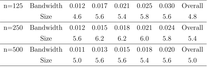
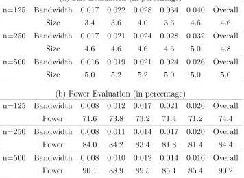
Tables 3 and 4 report the empirical size and power of the proposed test based on
B = 250 bootstrap resampled paths for each simulation. They contain the sizes and
powers for the overall test that is based on the five bandwidth set, and for the tests that
only use one bandwidth. We observe that the tests gave satisfactory sizes under both
testing settings. In the first test where we used the data from the jump diffusion model
VSK-MJ to test the continuous diffusion model VSK, the powers range from 65% to 95%
across the different sample sizes and bandwidths. In the second test where we used data
simulated from the infinity-activity jump process (the Inverse Gaussian OU) to test the
finite-activity jump process (the jump diffusion VSK-MJ), the powers range from 71% to
5
A Case Study
In this section, we examine empirically the capability of our testing procedure in detecting
jumps using the secondary market quotes of the 3-month Treasury Bill (T-bill) between
January 1, 1965 and February 2, 1999. This bill was sampled at monthly frequency, and
in total we had 410 observations. The mean of these bills is 0.065, the volatility is 0.026,
the mean of the differences is very close to zero (1.5×10⁻⁵) and the standard deviation
of the differences is 0.005. The sample period contains some large movements that turn
out to coincide with arrivals of macroeconomic news (Johannes (2004)). The goal of this
empirical study was to test whether the underlying process is subject to jumps or not.
The proposed parameter estimates under each of the four univariate models
consid-ered in the simulation study are reported in Table 5. For comparison, the MLEs or the
approximate MLEs are also reported except for the Inverse Gaussian OU model. For the
univariate diffusion models VSK and CIR, and the jump diffusion model VSK-MJ, the
proposed parameter estimates based on CCF are very similar to the MLEs or the
approx-imate MLEs. The EL estapprox-imates of the long-run mean α are 0.059 for VSK and 0.064 for
CIR, both of which are close to the summary statistic of mean rates (0.065). In VSK,
the average volatility of 3-month T-bill monthly return (difference) is estimated to be
σ√δ= 0.0181/12 = 0.005, which is also close to the summary statistic of volatility for the change (0.005). However the conditional volatility of monthly change in CIR model is
σ√δXt, and Xt has a long-run average 0.064 which is less than 1. Therefore, the process
needs to have higherσ (0.057) to bring up the average volatility of monthly change to the
same level reflected by the real data. In the jump diffusion model VSK-MJ, our estimate
of λ suggests on average about 2 jumps per year. Relative to VSK and CIR models, the
estimate for parameter σ in the jump diffusion VSK-MJ model is much smaller (0.008),
indicating that allowing jumps in the process helps capturing large movements in the
volatile as the one in VSK or CIR models.
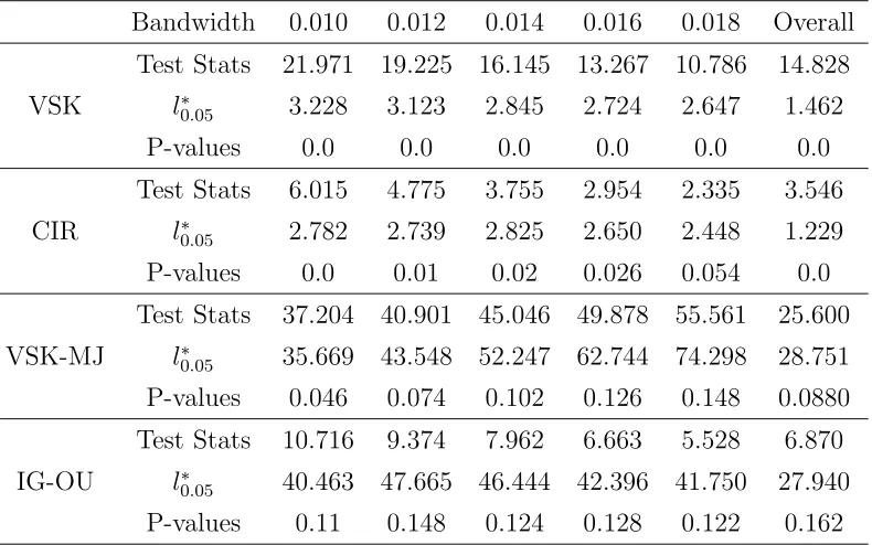
We then applied the proposed test for the validity of each of the four models. The
bandwidth prescribed by the CV was 0.01. By exploring the kernel estimators of the CCF,
a reasonable range for h was from 0.01 to 0.018, that offered smoothness from slightly
under-smoothing to slightly over-smoothing. The bandwidth range used in our empirical
study consisted of five equally spaced bandwidths ranging from 0.01 to 0.018. Table 6
reports p-values of single bandwidth and the overall tests for the four models. There is no
empirical support for VSK model. CIR model performs a little bit better as the distances
between the test statistics and the critical values decrease, but the model is still rejected
at significance level of 0.05 in the overall test and almost all the single bandwidth tests.
We can not reject the jump diffusion model VSK-MJ in the overall test and the single
bandwidth tests except the one with the smallest bandwidth (p-value = 0.046) . This
constitutes a strong evidence for the presence of jumps and implies that adding
(finite-activity) jumps does help capturing the underlying dynamics of the interest rates. By
allowing the infinite-activity jumps in the models, the p-values of the tests for the Inverse
Gaussian OU model are very supportive even for the small bandwidths, suggesting that
the infinite-activity jump model might potentially model the dynamics of the 3-month
T-bill rates better. A possible reason for it is that the jump diffusion model VSK-MJ can
only generate small continuous movements from Brownian motion and big spikes from the
compound Poisson component, but it could miss the movements that are between (i.e.
the movements with median sizes). However, the Inverse Gaussian OU process is more
flexible since it can generate small, median, and big movements with infinite arrival rates,
therefore it could fill in a gap in the VSK-MJ model by capturing movements that are
too large for Brownian motion to model but too small for the compound Poisson process
Appendix
The following conditions are required in our analysis.
C1: The stochastic processes given in (1.1) and (3.1) admit unique weak solution
respectively, which are α−mixing with mixing coefficient α(t) = Ce−λt where α(t) =
sup{|P(A∩B)−P(A)P(B)| : A ∈ Ωs
1, B ∈ Ω∞s+t} for all s, t ≥ 1, where C is a finite
positive constant and Ωji denotes the σ-field generated by {Xt :i≤t ≤j}.
C2: (Smoothness) ψt(τ;θ) =: ψ(τ;θ, Xt) and E{ǫt(τ;θ)} are third continuous
differ-entiable with respect to θ within a neighborhood of θ0 which is defined in C3. π(·) is
a bounded probability density supported on a compact set S ⊂ Rd; and the diffusion
function σ(x) is positive definite.
C3: The parameter space Θ is an open subset of Rp, and the true parameter θ
0 is the
unique root ofE{ǫt(τ;θ)}= 0 for allτ ∈S; and for anyθ1 =θ2,P {ψt(·;θ1)=ψt(·;θ2, Xt)}>
0.
C4: (Invertibility) The Hermitian matrix V ar{˜ǫt(τ;θ0)} is positive definite almost
everywhere for τ ∈ R2d with respect to the Lebesgue measure in R2d; Γ(θ
0) defined in
(2.9) is invertible.
C5: The kernel K(·) is a r-th order symmetric kernel supported on [−1,1]d and
has bounded second derivative. We assume d < 4 and the smoothing bandwidth h =
O{n−1/(d+2r)}. The bandwidth set {h
1,· · ·, hk} satisfies hi = cih for constants ci such
that c1 < c2 < ... < ck where k is an integer not depending on n.
C6: {∆n(u;Xt)}is a sequence of complex functions continuous atu= 0 and ∆n(0;Xt)≡
0, supn|∆n(u;Xt)| ≤M1 almost surely and the Lebesgue measure of {u|∆n(u, x)= 0} is
positive for all x in the support of the marginal density f, and cn =n−1/2h−d/4 which is
We need C1 as the basic condition for the stochastic processes involved. Ait-Sahalia
(1996) and Genon-Catalot, Jeantheau and Laredo (2000) provides conditions on the
un-derlying processes such that the Assumption C1 held. In particular, Ait-Sahalia (1996)
provides conditions so that the observed sequences are β-mixing, which is automatically
α-mixing. We require the rate of decay is exponentially fast to simplify the technical
arguments. C2 consists of smoothness conditions regarding the CCFs and C3 is for
iden-tification of parameters. C4 ensures the covariance matrix is invertible which is easier
to be justified for our low dimensional formulation of estimation and testing approaches.
C5 on the kernel and bandwidth are standard in non-parametric curve estimation. The
assumption of d <4 is to make the bias in the kernel estimation a smaller order of hd/2
so that the bias is stochastically negligible relative to ℓnh(θ0). The kernel method will
encounter the curse of dimensionality when d≥4. Also, the commonly used processes in finance and other stochastic modeling tend to have dimension less than 4. The bandwidth
selected by either cross validation or the plug-in method satisfies the order specified in
C5. The first part of C6 regarding ∆n(u;Xt) is to qualify ψt(u;θ) under H1 as a bona
fide characteristic function, whereas the part that requires positive measure on the set
{u|∆n(u, x)= 0} is to make H1 a genuine sequence of alternative hypotheses.
Proof of Lemma 1. By combining results in Kitamura (1997) and Chen, H¨ardle and Li
(2003) for the empirical likelihood of α−mixing processes, we can show that
λ(τ;θ) =An−1(τ;θ){1
n
n
t=1
ǫt(τ;θ)}+o(n−1/3) =O(n−1/3) (A.1)
follows from (A.1) and Taylor expansion that, uniformly in ||u||= 1,
ℓn(θ)
= {2n
t=1λT(τ;θ)ǫt(τ;θ)−nt=1{λT(τ;θ)ǫt(τ;θ)}2}π(τ)dτ +o(n1/3)
= n{1 n
n
t=1ǫTt(τ;θ0) + n1 nt=1 ∂ǫT
t(τ;θ0)
∂θ un
−1/3}A−1 n (τ;θ)
×{1 n
n
t=1ǫTt(τ;θ0) +n1 nt=1 ∂ǫT
t(τ;θ0)
∂θ un
−1/3}π(τ)dτ+o(n1/3)
= n{E(∂ǫT1(τ;θ0)
∂θ )un
−1/3(1 +o(1))}A−1(τ, τ;θ 0, θ0)
×{E(∂ǫ1(τ;θ0)
∂θ )un
−1/3(1 +o(1))}π(τ)dτ +o(n1/3)
≥ 1 2cn
1/3
(A.2)
almost surely, where c >0 is the smallest eigenvalue of
sup
τ∈SE(
∂ǫT 1(τ;θ0)
∂θ )A
−1(τ, τ;θ
0, θ0)E(
∂ǫ1(τ;θ0)
∂θ ).
Similarly,
ℓn(θ0) = {nt=1ǫTt(τ;θ0)}A−1(τ, τ;θ0, θ0){n1 nt=1ǫt(τ;θ0)}π(τ)dτ+o(1)
= o(n1/3) (A.3)
almost surely. This together with (A.2) implies that ℓn(θ) has a minimum value in the
interior of the ball ||θ−θ0|| ≤n−1/3 and this value satisfies ∂θ∂ ℓn(θ) = 0, i.e., the second
equation in (2.7) by noting (2.4). The first equation follows directly from (2.4).
Proof of Theorem 1. It follows from limit theorems for martingale difference that
⎧ ⎪ ⎪ ⎪ ⎪ ⎨ ⎪ ⎪ ⎪ ⎪ ⎩ ∂
∂θQ1n(τ;θ0,0) = 1 n
n
t=1 ∂θ∂ǫt(τ;θ0) p
→M0E{∂θ∂ ǫ˜1(τ;θ0)} ∂
∂λTQ1n(τ;θ0,0) = −
1 n
n
t=1ǫt(τ;θ0)ǫTt(τ;θ0) p
→ −M0A(τ, τ;θ0, θ0)M0⋆ ∂
∂θQ2n(τ;θ0,0) = 0 ∂
∂λTQ2n(τ;θ0,0) = n1 nt=1 ∂θ∂ǫTt(τ;θ0) p
→E{∂θ∂˜ǫ⋆
1(τ;θ0)}M0⋆
(A.4)
uniformly in τT ∈ S. Put δ
n = ||θˆn −θ0||+ supτT∈S||λ(τ; ˆθn)||. Then it follows from
Taylor expansion that
0 = Q1n(τ; ˆθn, λ(τ; ˆθn))
=Q1n(τ;θ0,0) + ∂Q1n∂θ(τ;θ0,0)(ˆθn−θ0) + ∂Q1n∂λ(τ;θT 0,0)λ(τ; ˆθn) +op(δn)
(A.5)
uniformly in τT ∈S, and
0 = Q2n(τ; ˆθn, λ(τ; ˆθn))π(τ)dτ
= {Q2n(τ;θ0,0) + ∂Q2n∂θ(τ;θ0,0)(ˆθn−θ0) + ∂Q2n∂λ(τ;θT0,0)λ(τ; ˆθn)}π(τ)dτ
+op(δn).
By (A.4) - (A.6), we have ˆ
θn−θ0
= −Γ−1(θ
0) E{∂θ∂ ˜ǫ⋆1(τ;θ0)}A−1(τ;θ0, θ0)M0−11n
n
t=1ǫt(τ;θ0)π(τ)dτ +op(δn).
(A.7)
Hence the theorem follows from (A.7) and the central limit theorem for Martingale
dif-ference.
Proof of Theorem 2. Define V(τ1, τ2, x;θ0, θ) =E{˜ǫ(τ1, Xt;θ)˜ǫ⋆(τ2, Xt;θ)|Xt =x} and
write V(τ, x;θ0, θ) =V(τ, τ, x;θ0, θ). Since ˆθn is √n-consistent to θ0, we have
ℓnh(ˆθn) = ℓnh,1(θ0) +nhdR−1(K){(ˆθ−θ0)TSn,h(θ0) +Sn,h⋆ (θ0)(ˆθn−θ0)
+(ˆθn−θ0)TΓn,h(θ0)(ˆθn−θ0)}+Op{(nhd)−1/2log3(n)
+h2log2(n)
}
(A.8)
where
ℓnh,1(θ0) = nhdR−1(K) ˜ǫn,h⋆ (τ, Xt;θ0)V−1(τ, x;θ0, θ0)
טǫn,h(τ, x;θ0)π1(τ)f−1(x)π2(x)dτ dx, (A.9)
Sn,h(θ0) = ∂˜ǫ⋆
n,h(τ,x;θ0)
∂θ V
−1(τ, x;θ
0, θ0)˜ǫn,h(τ, x;θ0)
×π1(τ)π2(x)f−1(x)dτ dx,
(A.10)
Γnh(θ0) = ∂˜ǫ⋆
n,h(τ,x;θ0)
∂θ V
−1(τ, x;θ
0, θ0)∂˜ǫn,h(τ,x;θ∂θ 0)
×π1(τ)π2(x)f−1(x)dτ dx.
(A.11)
As Sn,h(θ0) =Op(n−1/2),
ℓnh(ˆθn) = ℓnh,1(θ0) +Op{(nhd)−1/2log3(n) +h2log2(n) +hd}. (A.12)
Note that
ℓnh,1(θ0)
= nhdR−1(K)
n−1n
t1=1Kh(x−Xt1){ǫ˜
⋆(τ, X
t1) +cnη˜
⋆
n(τ, Xt1)}
×V−1(τ, x;θ
0, θ0)n−1nt2=1Kh(x−Xt2){˜ǫ(τ, Xt2) +cnη˜n(τ, Xt2)}
×π1(τ)π2(x)f−1(x)dτ dx+op(hd/2)
= R−1(K) (H
n1+Hn2+Hn3+Hn4) +op(hd/2),
(A.13)
where, with the choice of cn=n−1/2h−d/4,
Hn1 = n−1hdt1=t2
Kh(x−Xt1)Kh(x−Xt2)˜ǫ
⋆(τ, X t1)V
−1(τ, x)
טǫ(τ, Xt2)π1(τ)π2(x)f
−1(x)dτ dx,
Hn2 = n−1hdnt=1
K2
h(x−Xt)˜ǫ⋆(τ, Xt)V−1(τ, x)˜ǫ(τ, Xt)
×π1(τ)π2(x)f−1(x)dτ dx,
Hn3 = 2n1/2h3d/4 η˜n⋆(τ, x)V−1(τ, x)n−1
n
t=1Kh(x−Xt)˜ǫ(τ, Xt)
×π1(τ)π2(x)f−1(x)dτ dx,
Hn4 = hd/2 η˜n⋆(τ, x)V−1(τ, x)˜ηn(τ, x)π1(τ)π2(x)f−1(x)dτ dx.
We note thatHn2 = 2R(K) +op(hd) and and the integral inHn3 isOp(n−1/2). Hence,
Hn3 =Op(n3d/4) = op(hd/2).
Now considerHn1. Clearly,E(Hn1) = 0 and the double summation in Hn1 constitutes
a generalized U-statistic of order two with the kernel
ξt1,t2 =
Kh(x−Xt1)Kh(x−Xt2)˜ǫ
⋆(τ, X t1)V
−1(τ, x;θ
0, θ0)˜ǫ(τ, Xt2)
×π1(τ)π2(x)f−1(x)dτ dx. (A.15)
The U-statistic is degenerate due to{ǫ˜(τ, Xt2)} being martingale differences.
Let σ2
n =
1≤t1=t2≤nσt21,t2 where σ
2
t1,t2 = V ar(ξt1,t2). Then, apply the central limit
theorem for generalized U-statistics for α-mixing sequences (Gao and King, 2005), we
have
σ−1 n
t1=t2
ξt1,t2
d
→N(0,1). (A.16)
Furthermore, it can be shown, for instance by following the route of Chen, Gao and Tang
(2008) that σ2
n = 2n2σn02 {1 +o(1)} where σn02 =Et1Et2(ξ
2
t1,t2). Here Eti denote marginal
expectation with respect to (Xti, Xti+1).
It can be shown that
σ2
n0 =
Et1Et2{Kh(x1 −Xt1)Kh(x1−Xt2)Kh(x2−Xt1)
×Kh(x2 −Xt2)
2
l1,k1,l2,k2ǫl1(τ1, Xt1)ǫk1(τ1, Xt2)ǫl2(τ2, Xt1)
×ǫk2(τ2, Xt2)ν
l1,k1(τ
1, x1)νl2,k2(τ2, x2)}
×π1(τ1)π1(τ2)f−1(x1)f−1(x2)π2(x1)π2(x2)dτ1dτ2dx1dx2
=
Et1Et2{Kh(x1 −Xt1)Kh(x1−Xt2)Kh(x2−Xt1)
×Kh(x2 −Xt2)
2
l1,k1,l2,k2Vl1l2(−τ1, τ2, Xt1)Vk1k2(τ1,−τ2, Xt2)
×νl1,k1(τ
1, x1)νl2,k2(τ2, x2)}π1(τ1)π1(τ2)f−1(x1)f−1(x2)
×π2(x1)π2(x2)dτ1dτ2dx1dx2
= h−dγ2(K, V, π
1, π2){1 +O(h2)},
(A.17)
where γ2(K, V, π
1, π2) is defined in (3.4). From (A.16) and (A.17), we have
h−d/2Hn1 →d N(0,2γ2(K, V, π1, π2)) (A.18)
This together with the results on Hn2 and Hn3 leads to
where µn=Hn4. This completes the proof of Theorem 2.
Proof of Theorem 3. The proof can be made by applying the Cram´er-Wold device and
the same technique in the proof of Theorem 2 followed by the mapping theorem.
Acknowledgements:
The authors thank two reviewers and an associate editor for helpful comments, and
ac-knowledge support from National Science Foundation grants DMS-0604563, DMS-0518904,
SES-0631608 and DMS-1005336. The first author was partially supported through Center
for Statistical Science at Peking University.
References
[1] A¨ıt-Sahalia, Y. (1996). Nonparametric pricing of interest rate derivative securities.
Econometrica 64, 527–560.
[2] A¨ıt-Sahalia, Y. (2002), Maximum-likelihood estimation of discretely-sampled diffu-sions: a closed-form approximation approach. Econometrica 70, 223 – 262.
[3] A¨ıt-Sahalia, Y. (2008), Closed-form likelihood expansions for multivariate diffusions.
Ann. Statist. 36, 906 – 937.
[4] A¨ıt-Sahalia, Y., Fan, J. and Peng, H. (2009), Nonparametric transition-based tests for jump-diffusions. J. Amer. Statist. Asso. 104, 1102–1116.
[5] Barndorff-Nielsen, O. E. and Shephard, N. ( 2001), Non-Gaussian Orstein-Uhlenbeck-based models and some of their uses in financial econometrics. Journal of the Royal Statistical Society, Series B 63, 167 – 241.
[6] Carrasco, M., Chernov, M., Florens, J-P. and Ghysels, E. (2007), Efficient estimation of jump diffusion and general dynamic models with a continuum of moment conditions.
Journal of Econometrics 140, 529 – 573.
[7] Chacko, G. and Viceira, L. M. (2003), Spectral GMM estimation of continuous-time processes,Journal of Econometrics 116, no. 1-2, 259 – 292.
[8] Chen, B. and Hong, Y. (2010), Characteristic function-based testing for multifactor continuous-Time markov models via nonparametric regression. Econometric Theory26, 1115–1179.
[10] Chen, S. X., H¨ardle, W. and Li, M. (2003), An empirical likelihood goodness–of–fit test for time series. Journal of the Royal Statistical Society, Series B 65, 663 – 678.
[11] Chen, S. X. and I. Van Keilegom (2009), A review on empirical likelihood for regres-sions (with discusregres-sions), Test, 3, 415-447 .
[12] Chen, S. X., Peng, L. and Yu, C. L. (2011), Supplement to “Parameter Estimation and Model Testing for Markov Processes via Conditional Characteristic Functions”. DOI: XXXX.
[13] Cox, J. C., Ingersoll, J.E., and Ross, S.A. (1985), A theory of term structure of interest Rates. Econometrica 53, 385 – 407.
[14] Duffie, D., Pan, J. and Singleton, K. (2000), Transform analysis and asset pricing for affine jump-diffusions.Econometrica 68, 1343 – 1376.
[15] Fan, J. (2005), A selective overview of nonparametric methods in financial econo-metrics. Statistical Science20, 317 – 357.
[16] Feuerverger, A. (1990), An efficiency result for the empirical characteristic function in stationary time-series models. Canadian Journal of Statistics 18, 155 – 161.
[17] Feuerverger, A. and McDunnough, P. (1981), On some Fourier methods for inference. J. Amer. Statist. Asso. 76, 379 – 387.
[18] Feuerverger, A. and Mureika, R. A. (1977), The empirical characteristic function and its applications. Ann. of Statist. 5, 88 – 97.
[19] Genon-Catalot, V., Jeantheau, T. and Laredo, C. (2000). Stochastic volatility models as hidden Markov models and statistical applications. Bernoulli6, 1051C1079.
[20] Gao, J. and King, M. (2005), Estimation and model specification testing in non-parametric and seminon-parametric regression models. Unpublished paper available at www.maths.uwa.edu.au/˜jiti/jems.pdf.
[21] Jiang, G. J. and Knight, J. L. (2002), Estimation of continuous-time processes via the empirical characteristic function. Journal of Business and Economic Statistics 20, 198 – 212.
[22] Johannes, M. (2004), The statistical and economic role of jumps in continuous-time interest rate models. Journal of Finance 1, 227 – 260.
[23] Kitamura, Y. (1997), Empirical likelihood methods with weakly dependent processes. Ann. of Statist. 25, 2084 – 2102.
[24] Kitamura, Y., Tripathi, G. and Ahn, H. (2004), Empirical likelihood-based inference in conditional moment restriction models. Econometrica 72, 16671714.
[25] Merton,R. (1976), Option pricing when the underlying stock returns are discontinu-ous. Journal of Financial Economics3, 125 – 144.
[27] Owen, A. (1988), Empirical likelihood ratio confidence ratios for a single functional.
Biometrika 75, 237 – 249.
[28] Singleton, K. J. (2001), Estimation of affine asset pricing models using the empirical characteristic function.Journal of Econometrics 102, 111 – 141.
[29] Sørensen, M. (1991), Likelihood methods for diffusions with jumps. In Statistical Inference in Stochastic Processes,Ed. by Prabhu, N. U. and Basawa, I. V., 67 - 105.
[30] Strook, D. and Varadhan, S. (1979), Multivariate Diffusion Processes, Springer.
[31] Sundaresan, S. M. (2000), Continuous time finance: A review and assessment. Jour-nal of Finance 55, 1569 – 1622.
Table 1: Empirical averages and their standard errors (in parentheses) of the maximum (MLE) or approximate maximum (AMLE) likelihood estimates and the proposed empir-ical likelihood estimates (EL) under the four univariate models.
(a) Vasicek Model
n κ = 0.858 α = 0.089 σ = 0.047 125 MLE 1.383(0.603) 0.090(0.015) 0.047(0.003)
EL 1.305(0.643) 0.090(0.017) 0.046(0.004) 250 MLE 1.118(0.397) 0.090(0.011) 0.047(0.002) EL 1.052(0.410) 0.089(0.013) 0.046(0.002) 500 MLE 0.966(0.240) 0.089(0.008) 0.047(0.002) EL 0.951(0.273) 0.089(0.009) 0.047(0.002)
(b) CIR Model
n κ = 0.892 α = 0.091 σ = 0.181 125 MLE 1.372(0.644) 0.091(0.019) 0.183(0.012)
EL 1.290(0.719) 0.093(0.023) 0.178(0.014) 250 MLE 1.127(0.374) 0.090(0.013) 0.182(0.008) EL 1.089(0.435) 0.091(0.015) 0.179(0.009) 500 MLE 1.000(0.245) 0.091(0.010) 0.182(0.006) EL 0.977(0.290) 0.092(0.011) 0.180(0.007)
(c) Jump Diffusion VSK-MJ Model
n κ = 0.858 α= 0.089 σ = 0.047 λ= 2.0 η= 0.067 125 AMLE 1.056(0.381) 0.093(0.020) 0.046(0.005) 1.770(0.723) 0.060(0.016)
EL 1.090(0.261) 0.084(0.031) 0.048(0.009) 1.851(0.323) 0.066(0.020) 250 AMLE 0.977(0.226) 0.093(0.013) 0.047(0.003) 1.659(0.466) 0.059(0.010) EL 1.043(0.201) 0.090(0.023) 0.048(0.007) 1.825(0.236) 0.068(0.015) 500 AMLE 0.939(0.145) 0.092(0.009) 0.047(0.002) 1.620(0.311) 0.060(0.007) EL 1.018(0.115) 0.089(0.018) 0.049(0.005) 1.801(0.163) 0.068(0.012)
(d) Inverse Gaussian OU Model
Table 2: Empirical averages and their standard errors (in parentheses) of the maximum (MLE) likelihood estimates and the proposed empirical likelihood estimates (EL) under the Bivariate OU model.
n κ11 = 0.22 κ21 = 0.2 κ22= 0.5
125 MLE 0.441(0.197) 0.395(0.270) 0.607(0.176) EL 0.381(0.208) 0.525(0.238) 0.594(0.192) 250 MLE 0.353(0.165) 0.307(0.148) 0.563(0.110) EL 0.354(0.178) 0.449(0.184) 0.564(0.153) 500 MLE 0.280(0.118) 0.241(0.104) 0.526(0.068) EL 0.261(0.168) 0.383(0.154) 0.487(0.112)
n α1 = 0.08 α2 = 0.09 σ11 = 0.09 σ22 = 0.17
Table 3: H0: VSK versus H1: the jump diffusion model VSK-MJ
(a) Size Evaluation (in percentage)
n=125 Bandwidth 0.012 0.017 0.021 0.025 0.030 Overall Size 4.6 5.6 5.4 5.8 5.6 4.8 n=250 Bandwidth 0.012 0.015 0.018 0.021 0.024 Overall
Size 5.6 6.2 6.2 6.0 5.8 5.4 n=500 Bandwidth 0.011 0.013 0.015 0.018 0.020 Overall
Size 5.0 5.6 5.6 5.4 5.6 5.0
(b) Power Evaluation (in percentage)
n=125 Bandwidth 0.016 0.021 0.026 0.032 0.037 Overall Power 72.0 71.6 70.4 69.2 65.8 72.2 n=250 Bandwidth 0.016 0.019 0.022 0.026 0.029 Overall
Power 82.4 82.4 82.2 82.4 82.2 82.6 n=500 Bandwidth 0.014 0.017 0.019 0.021 0.024 Overall
Table 4: H0: the jump diffusion model VSK-MJ versus H1:the Inverse Gaussian OU
model
(a) Size Evaluation (in percentage)
n=125 Bandwidth 0.017 0.022 0.028 0.034 0.040 Overall Size 3.4 3.6 4.0 3.6 4.6 4.6 n=250 Bandwidth 0.017 0.021 0.024 0.028 0.032 Overall
Size 4.6 4.6 4.6 4.6 5.0 4.8 n=500 Bandwidth 0.016 0.019 0.021 0.024 0.026 Overall
Size 5.0 5.2 5.2 5.0 5.0 5.0
(b) Power Evaluation (in percentage)
n=125 Bandwidth 0.008 0.012 0.017 0.021 0.026 Overall Power 71.6 73.8 73.2 71.4 71.2 74.4 n=250 Bandwidth 0.008 0.011 0.014 0.017 0.020 Overall
Power 84.0 84.2 83.4 81.8 81.4 84.4 n=500 Bandwidth 0.008 0.010 0.012 0.014 0.016 Overall
Table 5: Empirical Estimation for the 3-month T-bill Data
(a) VSK Model
κ α σ
MLE 0.277 0.065 0.019 (0.1800) (0.0117) (0.0007) EL 0.274 0.059 0.018
(0.1956) (0.0136) (0.0007)
(b) CIR Model
κ α σ
MLE 0.182 0.066 0.061 (0.1697) (0.0179) (0.0021) EL 0.182 0.064 0.057
(0.1934) (0.0374) (0.0021)
(c) VSK-MJ Model
κ α σ λ η
AMLE 0.071 0.077 0.009 1.863 0.012 (0.0170) (0.0129) (0.0004) (0.3282) (0.0015) EL 0.072 0.076 0.008 1.862 0.013
(0.0143) (0.0136) (0.0008) (0.1569) (0.0021)
(d) Inverse Gaussian OU Model
λ a b EL 0.264 1.139 12.558
Table 6: P-values for the 3-month T-bill Data
Bandwidth 0.010 0.012 0.014 0.016 0.018 Overall Test Stats 21.971 19.225 16.145 13.267 10.786 14.828
VSK l∗
0.05 3.228 3.123 2.845 2.724 2.647 1.462
P-values 0.0 0.0 0.0 0.0 0.0 0.0 Test Stats 6.015 4.775 3.755 2.954 2.335 3.546 CIR l∗
0.05 2.782 2.739 2.825 2.650 2.448 1.229
P-values 0.0 0.01 0.02 0.026 0.054 0.0 Test Stats 37.204 40.901 45.046 49.878 55.561 25.600 VSK-MJ l∗
0.05 35.669 43.548 52.247 62.744 74.298 28.751
P-values 0.046 0.074 0.102 0.126 0.148 0.0880 Test Stats 10.716 9.374 7.962 6.663 5.528 6.870 IG-OU l∗
0.05 40.463 47.665 46.444 42.396 41.750 27.940