Munich Personal RePEc Archive
Semiparametric estimation of moment
condition models with weakly dependent
data
Bravo, Francesco and Chu, Ba and Jacho-Chavez, David
University of York, Carleton University, Emory University
2013
Online at
https://mpra.ub.uni-muenchen.de/79686/
Semiparametric Estimation of Moment Condition Models with
Weakly Dependent Data
Francesco Bravo∗
University of York
Ba M. Chu†
Carleton University
David T. Jacho-Ch´avez‡
Emory University
Abstract
This paper develops the asymptotic theory for the estimation of smooth semiparametric general-ized estimating equations models with weakly dependent data. The paper proposes new estimation methods based on smoothed two-step versions of the Generalized Method of Moments and Gen-eralized Empirical Likelihood methods. An important aspect of the paper is that it allows the first step estimation to have an effect on the asymptotic variances of the second-step estimators and explicitly characterizes this effect for the empirically relevant case of the so-called generated regressors. The results of the paper are illustrated with a partially linear model that has not been previously considered in the literature. The proofs of the results utilize a new uniform strong law of large numbers and a new central limit theorem for U-statistics with varying kernels that are of independent interest.
Keywords: Alpha-Mixing; Empirical Processes; Generalised Empirical Likelihood; Kernel
Smooth-ing; Stochastic Equicontinuity; Uniform Law of Large Numbers.
∗Department of Economics, University of York, Heslington, York YO10 5DD, UK. E-mail: [email protected].
Web Page: https://sites.google.com/a/york.ac.uk/francescobravo/.
†Department of Economics, Carleton University, B-857 Loeb Building, 1125 Colonel By Drive, Ottawa, ON K1S 5B6,
Canada. E-mail: ba [email protected]. Web Page: http://http-server.carleton.ca/ bchu/.
‡Corresponding Author: Department of Economics, Emory University, Rich Building 306, 1602 Fishburne Dr., Atlanta,
1
Introduction
In this paper we consider estimation of semiparametric statistical models defined by a set of gener-alized estimating equations. These models, often called over-identified moment conditions models in the econometric literature, are very general and contain semiparametric extensions to generalized in-strumental variable models used with economics and financial data and quadratic inference functions models used with longitudinal data. We develop two-step semiparametric extensions to the generalized method of moments (GMM) proposed by Hansen (1982), the generalized empirical likelihood (GEL) estimator of Newey and Smith (2004) and the exponentially tilted empirical likelihood (ETEL) esti-mator of Schennach (2007), where the first step is used to estimate an infinite dimensional nuisance parameters and the second-step is used to estimate a finite dimensional parameter of interest. The aforementioned methods have many desirable theoretical and practical properties. For example, GEL is a quasi-likelihood alternative to GMM that includes Owen’s (1988) Empirical Likelihood (EL), and
Kitamura and Stutzer’s (1997) Exponential Tilting (ET) as special cases. It does not require
estima-tion of the efficient metric as in GMM estimaestima-tion, and allows for the construcestima-tion of classical-type statistics such as likelihood ratio, and score for various hypotheses of interest. On the other hand GMM is computationally simpler than GEL, whereas ETEL is known to be robust to possible global misspecification of the estimating equations.
The theoretical properties of two-step semiparametric estimators have been considered both in the statistical and econometric literature for both cross section and time series data, see e.g. Truong and
Stone (1994), Andrews(1994a), Newey(1994), Gao and Liang (1997), Chen and Shen(1998), Li and
Wooldridge(2002),Chen et al.(2003) to name just a few among many others. Li and Racine(2007) and
Gao (2007) provide further examples and references. The statistical model we consider includes all of these models as special cases and in particular it allows for the possibility that the first-step estimation can affect the asymptotic variance of the second step estimator (the so-called estimation effect). To be specific we consider the case where the infinite dimensional parameter can depend on an estimated finite dimensional random vector. This case is empirically relevant because it often arises in situations where an estimated variable is used as a proxy for an unobservable variable of interest, such as for example the risk term in finance, and it is also theoretically interesting because with weakly dependent data the characterization of the estimation effect is more complicated. As far as we are aware of, this is the first paper that fully considers the estimation effect in semiparametric generalized estimating equations models with weakly dependent observations (seeMammen et al.,2015 andEscanciano et al.,
2014 for the case of just-identified semiparametric estimating equations models with independent and identically distributed (i.i.d.) observations).
The main methodological contribution of this paper is to derive the asymptotic properties of semi-parametric two-step GEL, GMM and ETEL estimators under the weakest form of dependency, namely
α (or strong) mixing (see for example Doukhan, 1994, for a review of statistical properties and ap-plications of α-mixing processes) using the same kernel based smoothing1 proposed by Kitamura and
Stutzer (1997) for ET and generalized by Smith (1997) (see also Smith, 2011) to GEL. In our
work, smoothing the estimating equations is useful whether there is an estimation effect or not. In the latter case smoothing is necessary for both the GEL and ETEL estimators to achieve the same asymptotic lower bound established by Chamberlain (1987) for efficient GMM estimators with i.i.d. observations. In the former case smoothing is useful because it results in heteroskedasticity and au-tocorrelation robust variance matrix estimators alternative to those typically used in both empirical economics and finance, see for exampleAndrews(1991). In this situation we obtain explicit formulae for the resulting asymptotic variance that are based on pathwise derivatives as in Newey (1994), and rely on a linear representation of the first-step estimator. This linear representation is fairly general and is satisfied, for example, in the important cases of non-parametric regression and non-parametric density estimators.
This paper also contains a number of new technical contributions that are used in the proof of the main results and are of independent interest. To be specific we establish a new strong uniform law of large numbers (SULLN) for strictly stationary α-mixing processes with a sharp logarithmic bound that depends on an exponential decay rate of theα-mixing coefficient, a weak condition on the growth rate of the bracketing entropy of a polynomial class of functions (of which Vapnik- ˇCervonenkis (V-C) classes are a special case), see e.g., van der Vaart and Wellner (1996, p. 86), and the existence of certain moments of the estimating equations. This result extends a number of ULLN available in both the econometric and statistical literature including those obtained byAndrews(1987),Yu(1993,
1994), Doukhan et al. (1994) andAdams and Nobel (2010). We also introduce two new central limit
theorems (CLT) (seeAppendix Bin the supplemental material) for both degenerate and nondegenerate second-order generalized U-statistics (that is U-statistics with varying kernels). The resulting CLTs are important because they represent a nontrivial extension of the existing results that are valid for either i.i.d. orβ-mixing sequences – see for example, de Jong(1987),Powell et al. (1989) and Mikosch
(1993) for the i.i.d. case, andYoshihara(1976,1989) and Fan and Li(1999) for theβ-mixing case. To establish these theorems, we impose mild regularity conditions directly on the kernel of theU-statistic and rely on Sun and Chiang’s (1997) conditional expectation bound for α-mixing sequences and on
Dvoretsky’s (1972) central limit theorem for double arrays of dependent random variables.2
The theoretical results of the paper are illustrated by deriving the asymptotic properties of an estimator of a general partially linear regression model, where we allow for the unobservable error to be correlated with the regressors and the infinite dimensional parameter to depend on an unknown finite dimensional parameter. Other examples where the results of the paper can be used are the weighted instrumental variable model that adapt for unknown heteroskedasticity ofRobinson (1987), the instrumental variable model of sample selection of Lee (1994), and the inverse-density-weighted moment model of Chu and Jacho-Ch´avez (2012) andChu et al. (2013).
The rest of the paper is organized as follows: The next section introduces the statistical model and the estimators. Section 3 contains the asymptotic results. Sections 4 and 5, respectively, introduce
2We note thatYoshihara (1992) uses an alternative approach to the one we follow to obtain the CLTs (and more
the new partially linear regression model and the results of the Monte Carlo simulations used to assess the finite sample properties of the proposed estimators. Section 6 contains some concluding remarks. The proofs of the theorems of Sections3and4are contained in theAppendix A. A supplement to this paper contains the new CLT’s for second-order generalizedU-statistics, a number of auxiliary technical lemmas and related proofs, which should be of independent interest.
The following notation is used in the text: a ” ′ ” denotes a matrix or vector transpose; for any finite dimensional possibly random vectorv or square matrixM,k · kdenotes the Euclidean norm and
kvkM := v′M v; for any measurable possibly vector valued function f(·), let kf(·)kp denote the Lp
norm, i.e., (Rkf(x)kpP(dx))1/p, and more generally for a pseudo-metric space, say H, k · k
H denotes a function norm, such as the sup norm.
2
The Model and Estimators
Let{zt, t= 1,2, ...} be a sequence ofZ-valued Z ⊂Rd weakly dependent random vectors defined on
a probability space (Ω,B, P). Let θ∈Θ⊂Rk denote the finite dimensional parameter of interest and
h∈ H denote the infinite dimensional nuisance parameter whereHis a pseudo-metric space. We consider a smooth semiparametric statistical model defined by
E[g(zt, θ, h)] = 0 iffθ=θ0 ∈int(Θ), and h=h0 ∈ H, (2.1)
where g(·) : Z ×Θ× H →Rl (l≥k) is a vector-valued measurable known function, and θ0 ∈int(Θ)
and h0 ∈ H are the true unknown parameters. As in Andrews(1994a), h is allowed to depend on zt
and possibly on a finite dimensional parameter α⊂A⊂Rp, so thath0 =: h0(zt, α0) includes also the
case of estimated random variables.
Let gt(θ, h) :=g(zt, θ, h); given a sample {zt}Tt=1 and a preliminary non-parametric estimator bh of
h0 a two-step GMM estimator θbforθ0 is defined as
b
θGMM = arg min
θ∈Θkgb(θ,bh)kWc, (2.2)
where bg(θ,bh) := T−1PT
t=1gt(θ,bh) and cW is a positive semi-definite possibly random Rl×Rl-valued
matrix that may depend on θ, and bh. The consistency of θbfollows by the results ofAndrews(1994a)
andChen et al.(2003), whereas its asymptotic normality follows by the results ofAndrews(1994a) with
weakly dependent observations under the assumption of asymptotic orthogonality - see Assumption 6
given below- and in full generality by the results of Chen et al.(2003) but only under the assumption of i.i.d. observations.
An alternative method for estimating θ0 is to use GEL and/or ETEL instead. To handle the
dependent structure of the estimating equation gt(θ, h), we follow the same approach ofSmith(1997)
and consider the following smoothed version
gts(θ, h) = 1
sT t−1 X
j=t−T
ω
j sT
wheresT is a bandwidth parameter andω(·) is a kernel function. Examples of possible kernel functions
include the Bartlett kernelωB(·) used for example byKitamura and Stutzer(1997) and the quadratic
spectral kernel ωQS(·) considered byAndrews(1991), given, respectively, by
ωB(x) = (
1− |x| ; |x| ≤1
0 ; otherwise, (2.3)
ωQS(x) =
25 12π2x2
sin (6πx/5) 6π/5 −cos
6πx
5
. (2.4)
Smith(2011) provides further examples and a detailed discussion of different choices ofω(·).
Let ρ(·) :Q→Rdenote a twice continuously differentiable function that is concave in its domain
Q - an open interval of the real line that contains 0. The smoothed two-step GEL criterion function for the semiparametric estimating equation satisfying (2.1) is
Γ (θ, h, λ) = 2
T
T X
t=1
[ρ(ωλ′gts(θ,bh))−ρ(0)],
where ω = ω1/ω2 (ωj := Rω(q)jdq, j = 1,2, . . .) is a normalization that has no effect on the GEL
estimator forθ0 but makes the scale of the estimator forλcomparable for different choices ofω(·) and
λis a vector of unknown auxiliary parameters.
The GEL estimator for θ0 is defined as the minimizer of the (profile) smoothed two-step GEL
criterion function, that is
b
θGEL= arg min
θ∈ΘΓ(θ,bh,bλ), (2.5)
where
b
λ:= arg max
λ∈ΛT
Γ(θ,bh, λ), (2.6)
for some fixedθand ΛT ={λ:λ′gts(θ,bh)∈Q}is the restricted parameter space ofλ(see for example
Newey and Smith,2004 and Smith,2011).
We can also define the following two-step smoothed GMM estimator for θ0,
b
θs-GMM= arg min
θ∈Θkbgs(θ, b
h)kcW, (2.7)
where bgs(θ,bh) := T−1PTt=1gts(θ,bh), which is an extension of that proposed by Smith (2005) and, as
opposed to the standard GMM estimator, takes directly into account the weakly dependent structure of the observations.3
3This implies that a consistent estimator of the efficient metricW = lim
T→∞var(T1/2bg(θ0, h0)) is given by an
appro-priately standardized version of the outer product of the smoothed estimating equationsgts(θ,bbh), viz.
"
1
sT TX−1
j=1−T ω
j
sT
2#−1
sT T
T
X
t=1
gts(θ,bbh)gts(θ,bbh)′− lim
T→∞var(T
1/2
b
g(θ0, h0))
=op(1),
The last estimator we consider is the two-step semiparametric ETEL estimator forθ0, that is defined
as
b
θETEL = arg min
θ∈Θ
1
T
T X
t=1
Tlogbπs(zt, θ,bh,λb), (2.8)
whereπbs(zt, θ,bh,bλ) =ρ1(ωλb′gts(θ,bh))/PTt=1ρ1(ωλb′gts(θ,bh)), and bλis as in (2.6) forρ(·) =−exp (·).
3
Asymptotic Theory
3.1 Strong Uniform Law of Large Numbers
We begin this section by introducing some further notation: LetF :={f(θ, h) : θ∈Θ, h∈ H}denote a class of functions indexed by an Euclidean parameter and an infinite dimensional parameter. Given a probability distribution P and F in Lp(P), let N[],p(ǫ, P,F) and H[],p(ǫ, P,F) denote, respectively,
the bracketing number and the ǫ-entropy with bracketing of F (see for example van der Vaart and
Wellner, 1996, Section 2.1, pp. 80-94)
Assumption 1 {zt, t= 1,2, . . .}is a sequence ofZ-valued Z ⊂Rd
stationary α-mixing random vec-tors with the mixing coefficient satisfying α(t) =O exp(−atb) for some positive aand b.
Assumption 2 The class of functions F satisfies
H[],1(ǫ, P,F) ≤υlog
1
ǫ
for some υ >0, (3.1)
E
"
sup
(θ,h)∈Θ×Hk
ft(θ, h)kµ #
<∞ for some µ≥4. (3.2)
Assumption 1 specifies the dependent structure of the observations as α-mixing. Examples of time series models that areα-mixing can be found inDoukhan (1994). α-mixing dependency is considered
byAndrews(1994a) in the context of semiparametric models, and byKitamura(1997) andSmith(2011)
in the context of EL and GEL estimation and inference for (finite dimensional) generalized estimating equations models. Assumption 1 imposes an exponential decay rate on the α-mixing coefficient α(t), which could be satisfied by many m-dependent stochastic processes, such as ARMA, GARCH, and bilinear processes; this same type of assumption has also been employed byBoente and Fraiman(1988)
andBonhomme and Manresa(2015) for example. Assumption2imposes a restriction on the complexity
of the class of functions F and the existence of some moments of order greater than 4. Various types of function classes such as H¨older, Sobolev and many others can be shown to satisfy (3.1) (see, e.g.,
van der Vaart and Wellner, 1996, Section 2.7, pp. 154-165). Note that (3.2) is only used to establish
the strong convergence rate in the following theorem.4
4Note that condition (3.1) combined with (3.2) forµ= 2 +ζ for some ζ >0 would suffice to prove a weaker version
Theorem 3.1 Under Assumptions 1 and 2
sup
(θ,h)∈Θ×H
1
T
T X
t=1
{ft(θ, h)−E[ft(θ, h)]}
=Oa.s.
logT Tβ
for some β∈
0,1
4
.
Remark 3.1 The proposed ULLN complements that of Yu (1993, 1994) who established a rate of convergence for a ULLN for strictly stationaryβmixing (absolutely regular) empirical processes indexed by a general class of functions with its capacity measured via the empirical metric entropy.
The above result is used repeatedly in the proofs of the Theorems 3.2 and 3.3. Its proof can be found in the supplemental material for this paper.
3.2 Asymptotic Normality
Let Θδ={θ∈Θ :kθ−θ0k ≤δ},Hδ ={h∈ H:kh−h0kH ≤δ}(possibly uniformly in α∈A), where
h:=h(zt) for some positive generic constant δ. Also let∂·denote a derivative operator with respect to
·, which corresponds to an ordinary partial derivative with respect to θ, and to the pathwise derivative in the direction ofh−h0, that is
∂g(zt, θ, h0)
∂h [h−h0] :=
∂g(zt, θ,(1−τ)h0+τ h)
∂τ |τ=0
(see Newey, 1994 for some examples). Assume that:
Assumption 3 (a) sT → ∞ as T → ∞, and sT = O(T
1
2−η) = o(T1/2) for some η ∈ 1
6,12
(cf.
Smith, 2011); (b) ω(·) : R→[−ω, ω] for some ω < ∞, ω(0) 6= 0, ω1 6= 0, ω(x) is continuous at 0 and almost everywhere, (2π)−1R−∞∞ exp (−ιxu)ω(x)dx ≥ 0 for each ω ∈ R and all u ∈ R, and R0
−∞supy≤x|ω(y)dx|+ R∞
0 supy≥x|ω(y)dx|<∞.
Assumption 4 (a) The class of functions G1 := {gt(θ, h) : θ ∈Θ, h ∈ H} satisfies conditions (3.1) and (3.2)in Assumption2; (b)Esupθ∈Θ,h∈Hδk∂θgt(θ, h)kα<∞andE[supθ∈Θδ,h∈Hδk∂hgt(θ, h)k
α]<
∞ for some α >2; (c) the class of functions G2 := {∂θhgt(θ, h) : θ ∈Θ, h ∈ H} satisfies conditions
(3.1) and (3.2) in Assumption2, E[supθ∈Θδ,h∈Hδ∂2
θθgt(θ, h) ]<∞.
Assumption 5 (a) kbh(zt)−h0(zt)kH=op T−1/4;
(b)bvT (θ, h) :=T−1/2PTt=1{gt(θ, h)−E[gt(θ, h)]}is stochastically equicontinuous at(θ0, h0)∈Θ×H.
Assumption3imposes some standard mild regularity conditions on the kernel functionω(·) used to smooth the observations and on the rate of growth of the related smoothing parameter sT. Note that
3.1. Assumptions 2, 3 and 4(a) can be used to show the consistency of the estimators described above. Assumption 5(a) assumes uniform consistency (possibly also with respect to α) of the non-parametric estimator used for h0. This is a standard assumption in the semiparametric literature of
two-step estimation procedures, see, e.g.,Chen et al.(2003),Escanciano et al.(2014,2016),Chen et al.
(2016), and Bravo et al. (2016). Similarly, Andrews (1995) provides sufficient conditions including the case of estimated random variables for kernel smoothing estimators. Assumption 5(b) is a high level assumption. It assumes stochastic equicontinuity of the empirical process bvT(θ, h). Although,
sufficient conditions for Assumption 5(b) are provided for example inAndrews(1994a,b), Lemma C.3
in the Appendix Cin the supplement provides a set of low level conditions that can be used to verify Assumption 5(b).
Assumption 6 (a) kE[gt(θ0,bh)]k =op T−1/2
; or (b) E[∂g(zt, θ, τ)/∂τ|τ=h0eh(zt)] = 0 ∀eh∈ H and z2t⊂zt.
Assumption 7 (a)bh(w)−h0(w) =T−1PTt=1ΦT (z2t, w)⊙φ(zt)+rT (w), where “⊙” is the Hadamard product, ΦT(z2t,·) is some weighting function, krT(w)kH =op T−1/2
(possibly uniformly in α∈A); (b)E[φ(zt)|Ft,z2t] = 0, where Ft,z2t is the minimum σ-algebra generated byz2t;E
φ(zt)φ(zt)′<∞; and limT→∞supwvar(T−(
1
2+δ)PT
t=1ΦT (z2t, w)⊙φ(zt))<∞ for some δ∈(0,1/2);
(c) the class of functionsG3 :={∂hh2 g(zt, θ0, h) :h∈ H}satisfies conditions (3.1)and (3.2) Assumption in 2.
Assumptions 6 and 7 account for the potential estimation effect from the first-step. When there is none, Assumption 6 implies the asymptotic orthogonality between the finite dimensional and the infinite dimensional parameter. In such case, it is not necessary to account for the presence of bh in the asymptotic distribution of θb, which greatly simplifies the calculation of the asymptotic variance. Condition 6(a) is directly assumed byAndrews(1994a), while Assumption6(b) is assumed byNewey
(1994). Note that forh=h(z2t) sufficient conditions for condition6(a) are Assumptions6(b) and5(a).
On the other hand, when there is estimation effect, Assumption 7 provides a generic way to account for it. For example, when h0 represents a conditional mean function, Assumption 7(a) requires that
the first-step estimator admits a certain asymptotic expansion which can be shown to hold when bh
represents some kernel-based non-parametric regression estimator of h0 (see for example Masry,1996
and Kong, Linton, and Xia, 2010); or bh := h(·,αb) when h0(·) = h(·, α0) is known up to some vector
of parameters α0. For instance, when bh is the Nadaraya-Watson estimator of h0 in a non-parametric
regression model, say z1t =h0(z2t) +ξt, then one can immediately show that Assumption 7(a) holds
under some regularity conditions with φ(zt) = z1t−h0(z2t) and ΦT(z2t, wt) = fz2t(wt)KbT(z2t−wt),
where fz2t(·) is the pdf of z2t and KbT(·) is a kernel function with bandwidthbT =b(T) that goes to
zero as T diverges to infinity.
Let Ω (θ0, h0) = limT→∞var T1/2gb(zt, θ0, h0), G(θ0, h0) = E[∂θg(zt, θ0, h0)] and Σ (θ0, h0) =
G(θ0, h0)′Ω (θ0, h0)−1G(θ0, h0).
Theorem 3.2 Assume that (a) θ0 ∈int(Θ), (b)Ω (θ0, h0) is positive definite, (c) rank(G(θ0, h0)) =k, (d) Σ (θ0, h0) is nonsingular, (e) kcW −Ω (θ0, h0)−1 k = op(1) for the GMM defined in (2.2) and s-GMM estimator defined in (2.7). Then under Assumptions 1-6 for θbdefined as in (2.2), (2.5), (2.7)
and (2.8)
T1/2(θb−θ0)→d N(0,Σ (θ0, h0)−1).
The following theorem establishes the asymptotic normality of the above estimator in the presence of estimation effect. Let
Ωed(θ0, h0) = lim T→∞var
"
1
T1/2 T X
t=2
gt(θ0, h0) + 1
(T −1)
t−1 X
s=1
Ψ (zs, zt, θ0, h0) !#
, (3.3)
Ωend(θ0, h0) = lim T→∞var
"
1
T1/2 T X
t=2
gt(θ0, h0) +h(1)T (zt, θ0, h0) !#
,
where
Ψ (zs, zt, θ0, h0) =∂hg(zt, θ0, h0)′ΦT (z2s, z2t)⊙φ(zs) +∂hg(zs, θ0, h0)′ΦT (z2t, z2s)⊙φ(zt) ,
h(1)T (·, θ0, h0) =E[Ψ (·, zt, θ0, h0)] = Z
Ψ (·, u, θ0, h0(u))fzt(u)du.
Theorem 3.3 Assume that (a) θ0 ∈int(Θ), (b) Ω (θ0, h0), Ωed(θ0, h0) and Ωend(θ0, h0) are positive definite, (c) rank(G(θ0, h0)) = k, (d) Σ (θ0, h0) is nonsingular. Then under Assumptions 1-5, and 7 for θbdefined in (2.5) or in (2.8)
T1/2(θb−θ0)→d N(0,Σ (θ0, h0)−1Σv∗(θ0, h0) Σ (θ0, h0)−1),
where
Σv∗(θ0, h0) =G(θ0, h0)′Ω (θ0, h0)−1Ωe∗(θ0, h0) Ω (θ0, h0)−1G(θ0, h0),
and Ωe
∗(θ0, h0) is either Ωed(θ0, h0) or Ωend(θ0, h0) given in (3.3).
For the two-step GMM estimator and its smoothed version, say θbℓ for ℓ∈ {GMM,s-GMM}, defined in
(2.2) and in (2.7) under (a)-(c) above, (d) Σe(θ
0, h0) is nonsingular and Assumptions 2-5, 7 and (e)
kcW −Ωe∗(θ0, h0)−1 k=op(1),
T1/2(θbℓ−θ0)→d N(0,Σe∗(θ0, h0)−1),
where
Remark 3.2 It is important to note that
Σe∗(θ0, h0)−1 ≤Σ (θ0, h0)−1Σv∗(θ0, h0) Σ (θ0, h0)−1
in the matrix sense,5 implying that in the presence of an estimation effect, as long as condition (e)
of Theorem 3.3 is satisfied, the two-step GMM estimator is more efficient than the smoothed two-step GEL or ETEL estimators. On the other hand, because of the explicit estimation of the efficient metric
Ωe∗(θ0, h0)−1both GMM estimatorsθbℓ forℓ∈ {GMM,s-GMM}might be more prone to bias. The Monte Carlo evidence of Section 5 based on the model considered in Section 4 seems to provide some support to both points.
4
Example: Partially Linear Instrumental Variable model
We consider a generalization of the partial linear model considered by Li and Wooldridge (2002)
yt=x′1tθ0+m0(x2t) +εt t= 1, . . . , T, (4.1)
where θ0 is an Rk-valued vector of unknown parameters, m0(·) is an unknown real valued function,
and the unobservable weakly dependent errors εt’s are such that E[εt|xt] = 0, where6 xt = [x′1t, x′2t]′.
Suppose that there exists an Rl-valued (l≥k) vector wt of instruments such that E(εt|x2t, wt) = 0;
then the estimation of the parameter of interest θ0 can be based on
gt(θ0, h0) =wt
yt−E(yt|x2t)−(x1t−E(x1t|x2t))′θ0
, (4.2)
whereh0:=h0(x2t) = [E(yt|x2t), E(x1t|x2t)′]′.
For vt = yt or x1t let Eb(vt|x2t) = PTs6=t=1vtKbT ((x2s−x2t)/bT)/
PT
s6=t=1KbT ((x2s−x2t)/bT),
where KbT(·) = K(·)/bT denotes a kernel estimator of the conditional expectation E[vt|x2t] with
bandwidthbT and let
gt(θ,bh) =wt eyt−xe′1tθ
,
whereyet=yt−Eb(yt|x2t),xe1t=x1t−Eb(x1t|x2t) denote the plug-in version of (4.2).
The following proposition establishes the asymptotic distribution of the two-step GMM, two-step GEL and two-step ETEL estimators when there is an estimation effect. To this end note that by the results ofAndrews(1994a) and Newey(1994), an estimation effect in (4.2) is only possible in the case of a generated regressor. So we assume that x2t is generated as a residual from the following linear
regression model st = vt′α0+x2t where α0 is a vector of unknown parameters and vt is a vector of
exogenous regressors so thatE[x2t|vt] = 0. We also note that because the model is linear in both the
finite and infinite dimensional parameters some of the regularity conditions (including a polynomial rate for the mixing coefficient α(t)) are weaker than those assumed in the theorems of the previous section.
5This follows since Σe(θ
0, h0)−Σ (θ0, h0) Σv∗(θ0, h0)−1Σ (θ0, h0) = X0′[I −Z0(Z0′Z0)
−1
Z′
0]X0 ≥ 0, for X0 =
Ωe
Proposition 4.1 Let zt := [yt, x′1t, x2t, w′t]′, and assume that: (a) {zt}Tt=1 is a sequence of α-mixing random vectors with α(t) = o t−2(2+γ); (b) the joint density f(zt) of zt and the marginal density
f(x2t) of x2t are twice continuously differentiable with bounded derivatives and infx2t∈X2∗f(x2t) > 0,
where X∗
2 is an open bounded subset of Rdx2 (c) h0(x2t) is twice continuously differentiable and
supx2t∈X∗
2 kh
(j)
0 (x2t)k < ∞ (j= 0,1,2) uniformly in A where h (j)
0 (·) is the jth derivative of h0(·); (d)Ekwt(yt−E(yt|x2t)−(x1t−E(x1t|x2t))′θ0)k4+γ <∞; (e) rank E
wt(x1t−E(x1t|x2t))′
=k, the matrices Ω (θ0, h0) and Ωe(θ0, h0) defined in (4.3) are positive definite; (f ) the function K(·) is a nonnegative second-order kernel with second order continuous bounded derivatives, and bT satis-fies T1/2b2
T → ∞, T1/2b4T → 0. Moreover
K(·+u)−K(u)−K(1)(·)u ≤ K(·)u2 where K(1)(·) is the first derivative of the kernel function and K(·) is a bounded function, (f ) T1/2(αb −α0) = PT
t=1r(vt)′x2t/T1/2 +op(1). Then the two-step GMM, GEL and ETEL estimators have the same distribution as that given in Theorem 3.3with
G(θ0, h0) =Ewt(x1t−E(x1t|x2t(α0)))′, (4.3)
Ω (θ0, h0) = lim T→∞var(T
−1/2 T X
t=1
wt[yt−E(yt|x2t(α0))−(x1t−E(x1t|x2t(α0)))θ0]),
Ωe(θ0, h0) = lim T−→∞var
(
1
T1/2 T X
t=1
wtεt+E
wt
f(x2t(α0))
∂α[f(x2t)h0(x2t(α0), θ0)]−
wt[h0(x2t(α0), θ0)]
f(x2t(α0))
∂αf(x2t(α0))
r(vt)′x2t(α0)
,
where h(x, θ) :=E[yt−x′1tθ|x2t=x] andx2t(α0) =st−v′tα0.
Proposition 4.1 generalizes some of the results of Li and Wooldridge (2002) to the possibly over-identified partial linear models withα-mixing errors. Note that in case of martingale difference errors, the above result simplifies to
Ω (θ0, h0) =E h
wtw′t(yt−E(yt|x2t(α0))−(x1t−E(x1t|x2t(α0)))θ0)2 i
,
Ωe(θ0, h0) = Ω (θ0, h0) +E
wt
f(x2t(α0))
∂α[f(x2t(α0))h0(x2t(α0), θ0)−h(x2t(α0), θ0)∂αf(x2t(α0)]
×
Er(vt)′r(vt)x22t(α0)E
wt
f(x2t(α0))
∂α[f(x2t(α0))h0(x2t(α0), θ0)−h0(x2t(α0), θ0)∂αf(x2t(α0)] ′
.
Letτ(x2t(α0)) :=I(x2t(α0)∈ X2∗) denote a fixed trimming function that equals one wheneverx2t(α0)∈
X2∗and zero otherwise; then given the results of Proposition (4.1) the proposed two-step semiparametric
functions
ΓGEL(θ,bh, λ) =
T X
t=1
τ(bx2t) [ρ(ωλ′gts(θ,bh))−ρ(0)],
ΓGMM(θ,bh, λ) =kτ(bx2t)bg(θ,bh)kΩbe(eθ,bh)−1,
Γs-GMM(θ,bh, λ) =kτ(bx2t)bgs(θ,bh)kΩbe(eθ,bh)−1,
ΓETEL(θ,bh, λ) = log
(
1
T
T X
t=1
τ(bx2t) exp[λ′gcts(θ,bh)] )
,
wherexb2t=x2t(αb) and Ωbe(eθ,bh) is a consistent estimator of Ωe(θ0, h0).
5
Monte Carlo Results
In this section we present results for the partial linear regression model with endogenous covariates in its parametric component discussed in Section 4. Specifically, we focus on
yt=x11tθ10+x12tθ20+m0(x2t) +εt,
x11t=π10v1t+π20v2t+ut,
wherev1t=ρ1v1t−1+ǫ1t,v2t=ρ2v2t−1+ǫ2t,εt=ρεεt−1+ǫεt,ut=ρuut−1+ǫut and "
ǫ1t
ǫ2t #
∼N
"
0 0
#
,
"
1 0 0 1
#!
,
"
ǫεt
ǫut #
∼N
"
0 0
#
,
"
1 ρεu
ρεu 1 #!
.
Letωlt∼N(0,1) (l= 2,3,4) independent ofv1tand v2t, and set x12t=v2t+ω2t,x2t=v1t+v2t+ω3t
such thatst=ω4tα0+x2t. Forρ1 =ρ2 = 0.5,ρε=ρu= 0.95, andm0(v) = Φ (v) (Φ (·) is the CDF of a
standard normal), we generate 2000 samples,{yt, x11t, x12t, st, ω4t, v1t, v2t}Tt=1, withT ∈ {200,400,800},
two different scenariosρεu ∈ {0.1,0.9}representing an increasing degree of endogeneity andθ0= [1,1]′,
π0 = [1,−1]′,α0 = 1.
Let zt := [yt, x11t, x12t,xb2t, v1t, v2t]′, wt := [x12t,xb2t, v1t, v2t]′, h0(zt) := [yet,xe11t,ex12t]′, yet := yt− b
E[yt|xb2t],xe11t:=x1t−Eb[x11t|xb2t], xe12t:=x12t−Eb[x12t|bx2t] andxb2t:=st−ω4tαb, so that
gt(θ,bh) =wt(yet−ex11tθ1−ex12tθ2),
where bh is the Nadaraya-Watson estimator with bandwidths chosen as c ∈ {0.5,1,1.5} times the Silverman’s rule-of-thumb bandwidth, andαb is an estimator of α0 obtained from regressing st on ω4t
by ordinary least squares.
Continuous Updated (CU) estimators; for the GMM estimators we use the following estimator
b
Ωe(θ,ebh) =
1
sT TX−1
j=1−T
ω2
j sT
−1 sT
T
τ(xb2t) T X
t=1
gts(θ,ebh)gts(θ,e bh)′, (5.1)
gts(θ,ebh) =
1
sT t−1 X
j=t−T
ω
j sT
(
wteεt+
1
T
T X
t=1 "
wt b
f(bx2t)
∂αfb(bx2t)hb(xb2t,θe)−
wt[bh(xb2t,θe)] b
f(xb2t)
∂αf(xb2t) #
b
r(ω4t)bx2t )
,
whereeεt=eyt−ex11tθe1−ex12tθe2,θe1 andθe2 are preliminary consistent estimators of θ10 andθ20,fb(bx2t) is
a kernel estimator of the marginal density ofxb2tand br(ω4t) =ω4t/PTt=1ω4t2/T
. In the Monte Carlo we use a Bartlett smoothing kernel with bandwidth parameter sT chosen by the method suggested
in Andrews(1991). The same bandwidths and kernels are used to estimate the asymptotic standard
errors based on (4.3) and to compute the estimator Ωbe(θ,ebh) given in (5.1).
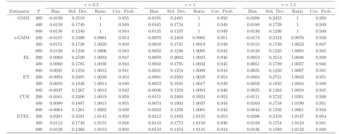
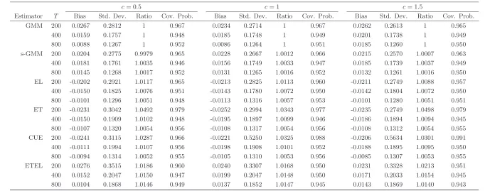
The Monte Carlo Bias (Bias), Standard Deviation (Std. Dev.), Average Ratios of Standard Errors (Ratio) with respect to that of a standard GMM and Coverage Probability (Cov. Prob.) are reported in Tables1-2for the estimator of the endogenous regressor parameterθ10. We use the standard GMM
partly because of its efficiency property discussed in Remark (3.2) and partly because it would probably be the most popular estimator given its (relatively) computational simplicity.
Tables 1 and 2 approx. here
We first consider the bias reported for the estimator of the endogenous regressor parameter and note that the bandwidth choice has some finite sample effect especially for T = 200 and 400, but it is also important to note that the magnitude of the bias of all of the proposed estimators is statistically insignificant. As expected, the degree of endogeneity has some negative effect on the bias for the smaller sample sizes. Second the standard and smoothed efficient GMM estimators are characterized by the largest bias but smallest standard deviations, whereas the EL estimator has the smallest bias, especially in the case of low endogeneity. Turning to the Monte Carlo standard deviation, we first note that in this case the degree of endogeneity have a less significant finite sample effect. Second the standard and smoothed GMM estimators seem to have an edge compared to the other estimators especially for
T = 200 and 400. Third, as pointed out in Remark3.2, the standard and smoothed GMM estimators have the smallest standard errors. Finally we note that the asymptotic approximation of all estimators seem appropriate for small samples as measured by the Monte Carlo coverage probability.
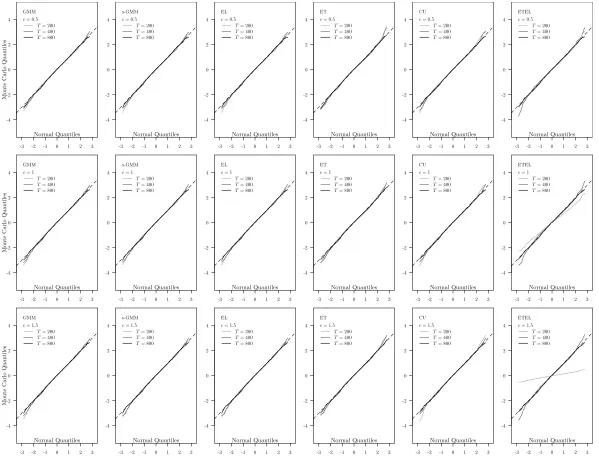
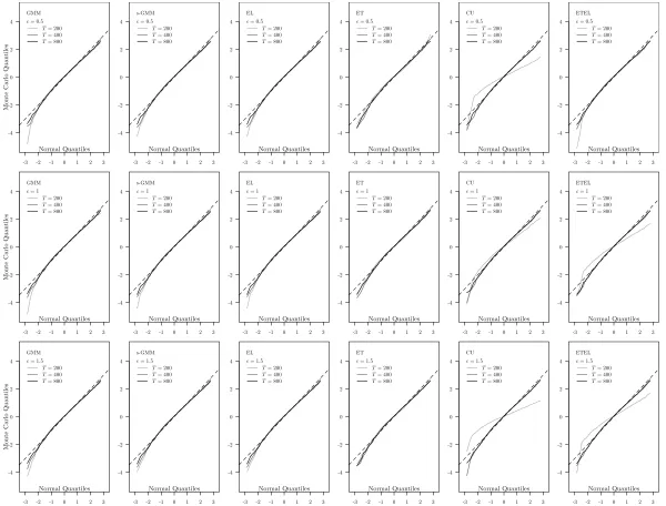
Figures 1-2 report the Q-Q plots that are used to illustrate the quality of the asymptotic normal approximation for the estimator of the exogenous regressor parameter θ20.
Figures 1 and 2 approx. here
The figures show that the asymptotic approximation is good across models especially for samples
improves with the sample size and seems to be robust to bandwidth choice for the first step estimator. Taking these results together, they suggest that the smoothed two-step estimators we are proposing seem to be characterized by good finite sample properties.
6
Conclusions
In this paper we consider the problem of estimating parameters of interest in semiparametric moment condition models with dependent data. We propose two-step GMM, GEL and ETEL estimators for the finite dimensional parameter and use smoothing to take the dependency into consideration. We show that as long as there is no estimation effect from the first step estimation all of the proposed esti-mators are asymptotically equivalent to the efficient GMM estimator of Hansen (1982). On the other hand, when there is estimation effect, this equivalence does not hold any longer for GEL and ETEL estimators, which become less efficient. Our proofs rely on a new uniform law of large numbers that generalizes that of Andrews’ (1987) and use two new CLT’s for both degenerate and non-degenerate second-order U-statistics with varying kernels. These results are of independent interest. We illus-trate the results with an instrumental variable partial linear model with a nonparametric generated regressor and use simulations to assess the finite sample properties of some of the proposed estima-tors. The results of the simulations suggest that overall all of the proposed estimators have good finite sample properties. Finally, we would like to mention that the results of this paper could be readily used in the context of quadratic inference functions for certain type of longitudinal data struc-tures {ziti, i= 1, ...n, ti= 1, ..., T}. In particular, under the additional assumption that the data are
independent and identically distributed across i for fixed ti, and are α-mixing with the same mixing
coefficient as that given in Assumption1 for a fixedi, it can be shown that the conclusion of Theorem
3.2is still valid for an appropriately smoothed version of the quadratic inference function g(ziti, θ, h).
The case for Theorem 3.3is considerably more complicated and we leave it for future research.
Acknowledgements
We thank an Associate Editor and two anonymous referees for various useful suggestions that improve the readability and clarity of the paper. We also acknowledge the usage of thenpandgmmpackages by
Hayfield and Racine(2008) andChauss´e(2010) respectively in the statistical computing environmentR.
Chu and Jacho-Ch´avez gratefully acknowledge support by the Social Science and Humanities Research Council of Canada grant (MBF Grant 410-2011-1700).
References
Andrews, D.W.K. (1987), ‘Consistency in Nonlinear Econometric Models: A Generic Uniform Law of Large Numbers’, Econometrica, 55, 1465–1471.
Andrews, D.W.K. (1991), ‘Heteroskedasticity and Autocorrelation Consistent Covariance Matrix Esti-mation’, Econometrica, 59, 817–858.
Andrews, D.W.K. (1994a), ‘Asymptotics for Semiparametric Econometric Models Via Stochastic Equicontinuity’, Econometrica, 62, 43–72.
Andrews, D.W.K. (1994b), ‘Empirical Process Methods in Econometrics’, inHandbook of Econometrics, Vol. IV, eds. R. Engle and D. McFadden. New York: North Holland, pp. 2247–2294.
Andrews, D.W.K. (1995), ‘Nonparametric Kernel Estimation for Semiparametric Models’,Econometric Theory, 11, 560–596.
Boente, G., and Fraiman, R. (1988), ‘Consistency of a Nonparametric Estimate of a Density Function for Dependent Variables’, Journal of Multivariate Analysis, 25, 90–99.
Bonhomme, S., and Manresa, E. (2015), ‘Grouped Patterns of Heterogeneity in Panel Data’, Econo-metrica, 83, 1147–1184.
Bravo, F., Chu, B.M., and Jacho-Ch´avez, D.T. (2016), ‘Generalized Empirical Likelihood M Testing for Semiparametric Models with Time Series Data’, Unpublished manuscript.
Chamberlain, G. (1987), ‘Asymptotic Efficiency in Estimation with Conditional Moment Restrictions’,
Journal of Econometrics, 34, 305–344.
Chauss´e, P. (2010), ‘Computing Generalized Method of Moments and Generalized Empirical Likelihood with R’, Journal of Statistical Software, 34, 1–35.
Chen, X., and Shen, X. (1998), ‘Sieve Extremum Estimates for Weakly Dependent Data’,Econometrica, 66, 289–314.
Chen, X., Linton, O., and van Keilegom, I. (2003), ‘Estimation of Semiparametric Models When the Criterion Function is Not Smooth’, Econometrica, 71, 1591–1608.
Chen, X., Jacho-Ch´avez, D.T., and Linton, O. (2016), ‘Averaging of an Increasing Number of Moment Condition Estimators’, Econometric Theory, 32, 30–70.
Chu, B.M., and Jacho-Ch´avez, D.T. (2012), ‘k-Nearest Neighbour Estimation of Inverse-Density-Weighted Expectations with Dependent Data’, Econometric Theory, 28, 769–803.
Chu, B.M., Huynh, K.P., and Jacho-Ch´avez, D.T. (2013), ‘Functionals of Order Statistics and their Multivariate Concomitants with Application to Semiparametric Estimation by Nearest Neighbors’,
de Jong, P. (1987), ‘A Central Limit Theorem for Generalized Quadratic Forms’, Probability Theory and Related Fields, 75, 261–277.
Doukhan, P. (1994), Mixing: Properties and Examples, Lecture Notes in Statistics, Vol. 85, New York: Springer & Verlag.
Doukhan, P., Massart, P., and Rio, E. (1994), ‘The Functional Central Limit Theorem for Strongly Mixing Processes’,Annales de L’Institut Henri Poincar´e (B) – Probabilit´es et Statistiques, 30, 63–82.
Dvoretsky, A. (1972), ‘Asymptotic Normality for Sums of Dependent Random Variables’, in Proceed-ings of the Sixth Berkeley Symposium on Mathematical Statistics and Probability, eds. L.M.L. Cam, J. Neyman, and E.L. Scott. University of California, pp. 513–535.
Escanciano, J.C., Jacho-Ch´avez, D.T., and Lewbel, A. (2014), ‘Uniform Convergence of Weighted Sums of Non- and Semi-parametric Residuals for Estimation and Testing’, Journal of Econometrics, 178, 426–443.
Escanciano, J.C., Jacho-Ch´avez, D.T., and Lewbel, A. (2016), ‘Identification and Estimation of Semi-parametric Two Step Models’, Quantitative Economics, 7, 561–589.
Fan, Y., and Li, Q. (1999), ‘Central Limit Theorem for DegenerateU-Statistics of Absolutely Regular Processes with Applications to Model Specification Testing’, Journal of Nonparametric Statistics, 10, 245–271.
Gao, J. (2007), Nonlinear Time Series: Semiparametric and Nonparametric Methods, Chapman and Hall/CRC.
Gao, J., and Liang, H. (1997), ‘Statistical Inference in Single-Index and Partially Nonlinear Models’,
Annals of the Institute of Statistical Mathematics, 49, 493–517.
Hansen, L.P. (1982), ‘Large Sample Properties of Generalized Method of Moments Estimators’, Econo-metrica, 50, 1029–1054.
Hayfield, T., and Racine, J.S. (2008), ‘Nonparametric Econometrics: The np Package’, Journal of Statistical Software, 27, 1–32.
Kitamura, Y. (1997), ‘Empirical Likelihood Methods with Weakly Dependent Processes’, Annals of Statistics, 25, 2084–2102.
Kitamura, Y., and Stutzer, M. (1997), ‘An Information Theoretic Alternative to Generalized Method of Moments Estimation’, Econometrica, 65, 861–874.
Lee, L. (1994), ‘Semiparametric Instrumental Variable Estimation of Simultaneous Equation Sample Selection Models’, Journal of Econometrics, 63, 341–388.
Li, Q., and Racine, J.S. (2007), Nonparametric Econometrics: Theory and Practice, Princeton Univer-sity Press.
Li, Q., and Wooldridge, J. (2002), ‘Semiparametric Estimation for Partially Linear for Dependent Data with Generated Regressors’,Econometric Theory, 18, 625–645.
Liebscher, E. (1998), ‘Estimation of the Density and the Regression Function under Mixing Conditions’,
Statistics & Decisions, 19, 9–26.
Mammen, E., Rothe, C., and Schienle, M. (2015), ‘Semiparametric Estimation with Generated Covari-ates’, Econometric Theory, 32, 1140–1177.
Masry, E. (1996), ‘Multivariate Local Polynomial Regression for Time Series: Uniform Strong Consis-tency and Rates’, Journal of Time Series Analysis, 17, 571–599.
Mikosch, T. (1993), ‘A Weak Invariance Principle for Weighted U-Statistics with Varying Kernels’,
Journal of Multivariate Analysis, 47, 82–102.
Newey, W.K. (1994), ‘The Asymptotic Variance of Semiparametric Estimators’, Econometrica, 62, 1349–1382.
Newey, W.K., and Smith, R.J. (2004), ‘Higher Order Properties of GMM and Generalized Empirical Likelihood Estimators’, Econometrica, 72, 219–256.
Owen, A. (1988), ‘Empirical Likelihood Ratio Confidence Intervals for a Single Functional’,Biometrika, 36, 237–249.
Powell, J., Stock, J., and Stoker, T. (1989), ‘Semiparametric Estimation of Weighted Average Deriva-tives’, Econometrica, 57, 1403–1430.
Robinson, P. (1987), ‘Asymptotically Efficient Estimation in the Presence of Heteroskedasticity of Unknown Form’, Econometrica, 55, 875–891.
Schennach, S. (2007), ‘Point Estimation with Exponentially Tilted Empirical Likelihood’, Annals of Statistics, 35, 634–672.
Smith, R.J. (1997), ‘Alternative Semi-Parametric Likelihood Approaches to Generalised Method of Moments Estimation’, Economic Journal, 107, 503–519.
Smith, R.J. (2005), ‘Automatic Positive HAC Covariance Matrix and GMM Estimation’, Econometric Theory, 21, 158–170.
Sun, S., and Chiang, C. (1997), ‘Limiting Behaviour of the Perturbed Empirical Distribution Functions Evaluated at U-Statistics for Strongly Mixing Sequences of Random Variables’, Journal of Applied Mathematics and Stochastic Analysis, 10, 3–20.
Truong, Y., and Stone, C. (1992), ‘Nonparametric Function Estimation Involving Time Series’,Annals of Statistics, 20, 77–97.
Truong, Y.K., and Stone, C.J. (1994), ‘Semiparametric Time Series Regression’,Journal of Time Series Analysis, 15, 405–428.
van der Vaart, A.W., and Wellner, J.A. (1996), Weak Convergence and Empirical Processes, New York, Berlin: Springer.
Yoshihara, K. (1976), ‘Limiting Behavior ofU-Statistics for Stationary, Absolutely Regular Processes’,
Probability Theory and Related Fields, 35, 237–252.
Yoshihara, K. (1989), ‘Limiting Behavior of Generalized Quadratic Forms Generated by Absolutely Regular SequencesII’, Yokohama Mathematical Journal, 37, 109–123.
Yoshihara, K. (1992), ‘Limiting Behavior of Generalized Quadratic Forms Generated by Regular Se-quences III’,Yokohama Mathematical Journal, 40, 1–9.
Yu, B. (1993), ‘Density Estimation in theL∞Norm for Dependent Data with Application to the Gibbs sampler’, Annals of Statistics, 21, 711–735.
Yu, B. (1994), ‘Rates of Convergence for Empirical Processes of Stationary Mixing Sequences’, Annals of Probability, 22, 94–116.
Appendix A
Main Proofs
Throughout this section “FOC” and “CMT” stand for, respectively, First Order Conditions and Continuous Mapping Theorem; unless otherwise stated “CLT” denotes a Central Limit Theorem for
α-mixing sequences (see for example Doukhan, 1994, Chapter 1.5). C and C(·) represent generic constants that may depend on additional quantities and may be different from line to line.
Proof of Theorem 3.1: See the supplemental material to this paper.
Proof of Theorem 3.2: We first show the consistency of θband bλ for the GEL criterion function. Without loss of generality we normalize the first two derivatives ρj(0) =−1 (j= 1,2) of ρ(·), where
ρj(0) :=∂jρ(q)/∂qj|q=0. Let ΛrT ={λ:kλk ≤RT} where RT =Op(sT/T)ξ forξ <1/2; as inSmith
(2011) it suffices to show that
sup
θ∈Θkb
gts(θ,bh)−ω1E[gt(θ, h0)]k=op(1) , (A-1)
max
1≤t≤Tλsup∈Λr T
sup
θ∈Θk
1 sT TX−1
t=1−T
ω
t sT
2!−1
sT
T
T X
t=1
gts(θ,bbh)gts(θ,b bh)′−Ω (θ0, h0)
=op(1) . (A-3)
To verify (A-1) note that by triangle inequality, Theorem 3.1 and dominated convergence
sup
θ∈Θkb
gs(θ,bh)−ω1E[gt(θ, h0)]k ≤
TX−1
j=1−T
1 sT ω j sT
θ∈Θ,hsup∈Hδ
1 T T X t=1
gt(θ, h)−E[gt(θ, h)] +
TX−1
j=1−T
1 sT ω j sT
−ω1
Eθ∈Θ,hsup∈Hδ
kgt(θ, h)k+
+ω1sup θ∈Θ
E[gt(θ,bh)]−E[gt(θ, h0)]
=op(1) ,
sincePTj=1−1−T sT−1ω(j/sT)−ω1
→ 0. To show (A-2) note that by triangle inequality and the (func-tional) mean value theorem one has
max
1≤t≤Tλsup∈Λr T
sup
θ∈Θk
λ′gts(θ,bh)k ≤RT
T−1 X
j=1−T
1 sT ω j sT × max
1≤t≤Tsupθ∈Θ "
kgt(θ, h0)k+ sup h∈Hδ
k∂hgt(θ, h)k kbh−h0kH
#
=op(1) ,
by Assumptions 4(a0-(b) and5(a) since max1≤t≤T supθ∈Θkgt(θ, h0)k=oa.s T1/µ and
max
1≤t≤Tsupθ∈Θhsup∈Hδk∂hgt(θ, h)k=oa.s
T1/2
by the Borel-Cantelli lemma. Finally, to show (A-3), it follows from the triangle inequality
sT T T X t=1
gts(θ,bbh)gts(θ,bbh)′−ω2Ω (θ0, h0) ≤ sT T T X t=1
gts(θ0, h0)gts(θ0, h0)′−ω2Ω (θ0, h0) + 2 sT T T X t=1
gts(θ0, h0) [gts(θ,bbh)−gts(θ0, h0)]′ + sT T T X t=1
[gts(θ,bbh)−gts(θ0, h0)][gts(θ,b bh)−gts(θ0, h0)]′ =T ∗
1+T∗2+T∗3.
T∗1 =op(1) by Lemma A.3 ofSmith(2011). Calculations along the lines of Lemma A.3 ofSmith(2011)
and Cauchy-Schwarz inequality yield
T∗2 ≤
1 sT TX−1
s=1−T
ω
t−s sT ω t sT
kbg(θ0, h0)k2kbg(θ,bbh)−gb(θ0, h0)k2+O
t T
,
and by the functional mean value theorem, Assumptions4and 5(a)
1 T T X t=1
gt(θ,bbh)−gt(θ0, h0)
2 ≤ kbh−h0k2H sup
θ∈Θδ,h∈Hδ
1 T T X t=1
k∂hgt(θ, h)k2
hence T∗
2=op(1) since
lim
T→∞
1
sT TX−1
t=1−T
t Tω
t−s sT
ω
t sT
= 0
by Lemma C.1 of Smith(2011). Similar arguments yield T∗
3 =op(1). Clearly Pr (ΛrT ∈ΛT) → 1 and
note that by (A-2) and CMT
sup
θ∈Θ,λ∈Λr T
max
1≤t≤T
ρj(λ′gts(θ,bh))−ρj(0)
=op(1) , j= 1,2. (A-4)
Given (A-1)-(A-4), the consistency of the GEL estimator bθ follows by the same arguments of Newey
and Smith(2004) andSmith(2011). First note that
sup
λ∈Λr T
1
sT
Γ(θ0,bh, λ)≤ kbgs(θ0, h0)k2+
1
sT h
Γ(θ0,bh, λ)−Γ (θ0, h0, λ) i
, (A-5)
and that by a Taylor expansion along the continuous connected path h∗(ǫ) =h0+ǫ(bh−h0) such that
h∗(ǫ)∈ Hδ,∀ǫ∈[0,1] we have
Γ(θ0,bh, λ) = Γ (θ0, h0, λ) +ω(1−ǫ)
1
T
T X
t=1
ρ1 ωλ′gts(θ0, h∗(ǫ))
λ′∂hgts(θ0, h∗(ǫ)) (bh−h0),
whereǫ∈(0,1). Then by triangle inequality
Γ(θ0,bh, λ)−Γ (θ0, h0, λ) ≤
(1−ǫ)ω
1
T
T X
t=1
λ′∂hgts(θ0, h∗(ǫ)) (bh−h0) +
(1−ǫ)ω
1
T
T X
t=1
ρ1 ωλ′gts(θ0, h∗(ǫ))−ρ1(0)λ′∂hgts(θ0, h∗(ǫ)) (bh−h0) ≤
RTkbh−h0 kH sup
h∈Hδ
1
T
T X
t=1
k∂hgts(θ0, h)k λ∈Λsupr
T,h∈Hδ
ρ1 ωλ′gts(θ0, h)
−ρ1(0)
=op(1)
by Assumptions4and5(a). LetλT =−bg(θ,b bh)ξT/kgb(θ,bbh)kwhere|ξT|< RT, so that Pr (λT ∈ΛrT)→
1. A Taylor expansion of Γ(θ,bbh, λT) with respect toλT′ gts(θ,bbh) about 0 gives
Γ(bθ,bh, λT)≥ −ωλ′Tbgs(θ,bbh)−Cω2λ′TλT =ωξTkbg(θ,bbh)k −Cω2ξ2T.
Since
Γ(θ,bbh, λT)≤ sup λ∈Λr T
Γ(θ,bbh, λ)≤ sup
λ∈Λr T
Γ(θ0,bh, λ),
we have by (A-5), the CLT and some algebra yield
kbg(θ,bbh)k ≤ sT
ξT kb
g(θ0, h0)k2+op(1) =o
T1/2Op T−1
,
kbg(θ,b bh)k =op(1). The consistency of θbfollows now by Lemma C.1and the identification condition
(2.1). A similar expansion can be used to show thatkλbk=Op sT/T1/2whereλb= arg maxλ∈Λr
T Γτ(θ,bbh, λ).
The asymptotic distribution is obtained by a standard mean value expansion of the FOC
that hold with probability →1 by (a), and gives
T1/2[(θb−θ0)′,bλ/sT]′ =
1
ω1 c
M(λ, θ,bh)−1[0′,−T1/2gbs(θ0,bh)′]′+op(1) ,
where
c
M(λ, θ,bh) =
"
0 T1 PTt=1ρ1(ωλ
′
gts(θ,bh))∂θgts(θ,bh) 1
T PT
t=1ρ1(ωλ′gts(θ,bh))∂θgts(θ,bh) sTT Ptρ2(ωλ′gts(θ,bh))gts(θ,bh)gts′ (θ,bh) # . Note that 1 T T X t=1 h
ρ1(ωλ
′
gts(θ,bh))−ρ1(0) i
∂θgts(θ,bh) +ρ1(0)
1
T
T X
t=1
∂θgts(θ,bh)≤
sup
λ∈Λr T,h∈Hδ
ρ1 ωλ′gts(θ0, h)−ρ1(0) 1 T T X t=1
∂θgts(θ,bh) + 1 T T X t=1
∂θgts(θ,bh)−
1
T
T X
t=1
∂θgts θ, h0 , and 1 T T X t=1
∂θgts(θ,bh)−
1
T
T X
t=1
∂θgts θ, h0
≤ kbh−h0kH sup
θ∈Θδ,h∈Hδ
1 T T X t=1
∂θh2 gts(θ, h)
=op(1) .
Thus by (A-5), Theorem 3.1, condition 5(a) and the CMT
1
T
T X
t=1
ρ1(ωλ
′
gts(θ,bh))∂θgts(θ,bh) p
→ω1E[∂θgt(θ0, h0)] .
Similarly note that
sup
λ∈Λr T,h∈Hδ
ρ2 ωλ′gts(θ0, h)
−ρ2(0)
=op(1) , (A-6)
and sT T T X t=1
ρ2(ωλ′gts(θ,bh))gts(θ,bh)gts(θ,bh)′−
sT
T
T X
t=1
ρ2(0)gts(θ0, h0)gts(θ0, h0)′
(A-7)
≤θ−θ0 "
1
T θ∈Θsupδ,h∈Hδ
T X
t=1
kgt(θ, h)k2 #1/2"
1
T θ∈Θsupδ,h∈Hδ
T X
t=1
k∂θgt(θ, h)k2 #1/2
+
kbh−h0 kH
"
1
T θ∈Θsupδ,h∈Hδ
T X
t=1
kgt(θ, h)k2 #1/2"
1
T θ∈Θsupδ,h∈Hδ
T X
t=1
k∂θgt(θ, h)k2 #1/2
p
→0,
so that by (A-3), ksTT−1Ptρ2(ωλ′gts(θ,bh))gts(θ,bh)gts(θ,bh)′−Ω (θ0, h0)k=op(1). Thus by triangle
inequality and the CMT
c
M(λ, θ,bh)−1 →p
"
Σ (θ0, h0) H(θ0, h0)
H(θ0, h0)′ P(θ0, h0) #
where
H(θ0, h0) = Σ (θ0, h0)G(θ0, h0)′Ω (θ0, h0)−1
P(θ0, h0) = Ω (θ0, h0)−1 h
I −G(θ0, h0) Σ (θ0, h0)G(θ0, h0)′Ω (θ0, h0)−1 i
.
Then by Assumptions 5(b) and6(a) we have
T1/2[(θb−θ0)′,bλ′/sT]′ = 1
ω1
M(θ0, h0)−1 h
0′,−T1/2ω1bg(θ0, h0)′ i′
+op(1) (A-8)
and by CLT and CMT
T1/2[(θb−θ0)′,λb′/sT]′→d N(0,diag [Σ (θ0, h0), P(θ0, h0)]) .
The consistency of the two step smoothed semiparametric GMM based estimator θb, in (2.7), follows by the identification condition (2.1), and the uniform convergence of kbgs(θ,bh)kWc, which follows by (A-1), kWc−W k=op(1) for any positive definite matrixW, and
kbgs(θ,bh)kcW − kω1E[gt(θ, h0)]kW
≤ kgbs(θ,bh)−ω1E[gt(θ, h0)]k2kWc k+
kω1E[gt(θ, h0)]k kWc−W k+ 2kω1E[gt(θ, h0)]k ×
kbgs(θ,bh)−ω1E[gt(θ, h0)]k kWck=op(1) ,
by the triangle inequality. The asymptotic normality follows by a standard Taylor expansion aboutθ0
of the FOC
0 =T1/2[∂θbgs(θ,bhb)]cWbgs(θ,b bh)
that hold with probability → 1 by assumption (a). The conclusion follows by (2.1) (applied to
∂θbgs(zt, θ,bh)), assumption 5(b), CLT and CMT. The consistency of the two-step smoothed
semipara-metric ETEL estimatorθbfollows by a two step argument: First, for anyλsuch that Pr λ∈ΛrT→1, the same arguments as those used to show the consistency of the GEL estimator show that the ETEL estimator
b
θ= arg min
θ∈Θλsup∈Λr T
log
(
1
T
T X
t=1
exp{ωλ′[gts(θ,bh)−bgs(θ,bh)]} )
(A-9)
is consistent. Next the consistency of bλdefined as
b
λ:= arg max
λ∈Λr T
1
T
T X
t=1
−exp{ωbλ′gts(θ,bh)}
follows noting that by a second order Taylor expansion about 0, (A-4) and (A-6) we have
0≤1− 1
T
T X
t=1
exp{ωbλ′gts(θ,bbh)} ≤ 1−
1
T
T X
t=1
exp{ωbλ′gts(θ0,bh)}=
ωbλ′bgs(θ0,bh) +
ω2
2 λb ′ sup
h∈Hδ
T X
t=1
ρ2 ωλˇ′gts(θ0, h)gts(θ0, h)gts(θ0, h)′bλ≤
where the last inequality follows by the triangle inequality, a similar argument as that used in (A-7) andT−1PTt=1ρ2(ωλˇ′gts(θ0, h))gts(θ0, h0)gts(θ0, h0)≤ −CI (Smith,2011, p. 1224). By condition5(b)
and the CLT kbgs(θ0,bh)k=O T−1/2
hencekbλk =Op sTT−1/2
. Thus Pr(bλ∈ΛrT) →1, which in turn implies the consistency of bθ given in (A-9) with bλ=λ. The asymptotic normality follows using the same Taylor expansion and the same arguments as those used to obtain (A-8) (see alsoSchennach,
2007).
Proof of Theorem3.3: The consistency ofθbandbλfollows by the same arguments as those used in the proof of Theorem3.2, so we assume consistency and derive the asymptotic distribution of T1/2(θb−θ0).
By a Taylor expansion with Cauchy remainder
gt(θ0,bh) =gt(θ0, h0) +∂hgt(θ0, h0) (bh−h0) +1
2
Z 1
0
∂2hhght(θ0, h0+ξ(bh−h0))dξ,
where∂hh2 gth(·) =Plh
j=1(bh−h0)j∂hh2 jgt(·) (bh−h0)
′, so that by Assumption7it follows that
T1/2bgs(θ0,bh) =T1/2bg(θ0, h0) +
1
T3/2 T X
t=1
1
sT t−1 X
s=1−T
ω
s sT
∂hgt−s(θ0, h0)×
T X
τ=1,τ6=t
ΦT(z2t, z2t−τ)⊙φ(zt) +
1
T3/2 T X
t=1
1
sT t−1 X
s=1−T
ω
s sT
rT (z2t−s) +
1
T3/2 T X
t=1
1
sT t−1 X
s=1−T
ω
s sT
Z 1
0
∂hh2 ght(θ0, h0+ξ(bh−h0))dξ
:=T∗
4+T∗5+T∗6+T∗7.
By CLT T∗4→d N 0, ω21Ω (θ0, h0) whereas by Assumption 7(a) and Lemma C.1 ofSmith(2011)
lim
T→∞ 1
sT TX−1
s=1−T ω
s sT
krT(Tz2t1/2−s)kH =op(1).
The term T∗
5 can be written as
T∗5= 1
sT T−1 X
s=1−T
ω
s sT
1
T3/2
min(T,TX−s)
t=max(1,1−s) T X
τ=1,τ6=t
∂hgt−s(θ0, h0) ΦT (z2t, z2t−τ)⊙φ(zt)
:= 1
sT TX−1
s=1−T
ω
s sT
UT,s, (A-10)
inequality yields
P
1
T3/2
s X
t=1 T X
τ=1,τ6=t
∂hgt−s(θ0, h0) ΦT(z2t, z2t−τ)⊙φ(zt) ≥ǫ
≤
1
ǫT3/2 s X
t=1 T X
τ=1,τ6=t
E|∂hgt−s(θ0, h0) ΦT (z2t, z2t−τ)⊙φ(zt)| ≤
1
ǫT3/2 s X
t=1
k∂hgt(θ0, h0)k2sup z2t
T X
τ=1
ΦT (z2t, z2t−τ)⊙φ(zt) 2
≤O
|s| T1−δ
,
where the last equality follows from Assumptions7(b)-(c). It then follows that
P
1
sT TX−1
s=1−T
ω
s sT
{UT,s−UT} > ǫ
!
≤ 1ǫs1
T TX−1
s=1−T
ω
s sT
E|UT,s−UT| (A-11)
≤CTδ 1 sT
TX−1
s=1−T
|s| T
ω
s sT
=O(Tδ−η−1/2) =o(1),
where the last equality follows from Lemma C.1 ofSmith(2011).6 Thus by (A-10) and (A-11)
T5∗= (ω1+o(1))√T UT∗+O(Tδ−η−1/2),
where UT∗ := PTt=1PTs=1,s6=tΦeT(z2s, z2t)/T(T−1) and ΦeT(z2s, z2t) = ∂hgt(θ0, h0) ΦT (z2s, z2t) ⊙
φ(zs). SinceUT∗ can be represented as a U-statistic with a varying symmetric kernel, that is
UT∗ = 1
T(T−1)
X
1≤s<t≤T
ΨT (z2s, z2t) ,
where ΨT (z2s, z2t) := ΦeT (z2s, z2t) +ΦeT(z2t, z2s), the asymptotic normality of T1/2UT∗ follows by
ei-ther Lemma B.1 or B.2, so that the asymptotic normality of T1/2gbs(θ0,bh) follows by the CMT as
long as kT∗
7k = op(1). Note that Theorem 3.1 and A7(c) yield suph∈Hδ
PT
t=1∂hh2 gt(θ0, h)/T a.s.→
E[suph∈Hδ∂2
hhgt(θ0, h)], which implies that
1
T
T X
t=1
Z 1
0
(1−ξ)∂hh2 gt(θ0, ξ(h−h0))dξ
=Oa.s.(1).
Thus kT∗
7k = op(1) follows by Assumption 5(a) and the CMT. The asymptotic equivalence between
the GEL estimatorθbdefined in (2.5), and the ETEL estimatorθbdefined in (2.8) implies that the latter has the same asymptotic covariance as that of the former. Finally for the GMM estimator θbdefined in (2.7), the result follows by the above arguments and those used in the proof of Theorem 3.2 using the metricΩbe(θ,ebh)−1, Assumption (e) and the CMT.
6In fact Lemma C.1 inSmith(2011) states that lim
T→∞s−1T PtT=1−−1T|t|T−1|ω(t/sT)|= 0. However, an examination
of the proof reveals that, actually,s−1
T
PT−1
t=1−T|t|T
Proof of Proposition 4.1: Note that by the consistency ofαb
T1/2bgs(θ0,bh(bx2t))τ(bx2t) =T1/2bgs(θ0,bh(xb2t)) (τ(xb2t)−τ(x2t)) +T1/2gbs(θ0,bh(xb2t))τ(x2t)
=T1/2bgs(θ0,bh(xb2t))τ(x2t) +op(1)
and
T1/2bgs(θ0,hb(xb2t))τ(x2t) =T1/2ω1bg(θ0, h(x2t, θ0))τ(x2t)−
ω1
T1/2 T X
t=1
wt[bh(x2t, θ0)−h(x2t, θ0)]τ(x2t)−
ω1
T1/2 T X
t=1
wt[bh(xb2t, θ0)−bh(x2t, θ0)]τ(x2t)
:=Tg;1+Tg;2+Tg;3,
where bh(·) is a kernel estimator for h(·), xb2t =st−vt′αb is the regression residual and, for notational
simplicity, for x2t(α0) = st−vt′α0, x2t(α0) := x2t The asymptotic normality of Tg;1 follows by CLT;
furthermore Tg;2=op(1) by an application of the Cauchy-Schwartz inequality, a covariance inequality
forαmixing processes (see e.g., Truong and Stone,1992), a standard law of large numbers and results
of Liebscher(1998), which show that
var (Tg;2)≤sup t E
h
|bh(x2t, θ0)−h(x2t, θ0)|2τ(x2t) iω
1
T
T X
t=1
wtw′t
+ sup
t
Eh|bh(x2t, θ0)−h(x2t, θ0)|2τ(x2t) i2 ω1
T
T X
s6=t
E[wswt′]
=O
sup
t
Eh|bh(x2t, θ0)−h(x2t, θ0)|2τ(x2t) i
→0
ForTg;3 sincex2tis estimated parametrically we have the following linear representation:
b
h(bx2t, θ0)−bh(x2t, θ0) =
1
DT(x2t, θ0)
(1−DT(xb2t, θ0)[DT(bx2t, θ0)−DT(x2t, θ0)])
NT(xb2t, θ0)−NT(x2t, θ0)−
NT(x2t, θ0)
DT(x2t, θ0)
[DT(bx2t, θ0)−DT(x2t, θ0)]
,
where DT(x2t, θ) : =T−1PTs6=tKbT(x2s−x2t), NT(x2t, θ) : =T
−1PT
s6=t(ys −x′1tθ)KbT(x2s−x2t),
KbT(x2s−x2t) := K((x2s−x2t)/bT)/bT , K(·) is a kernel function andbT is the bandwidth. Then
again by the results ofLiebscher (1998) we have
b
h(bx2t, θ0)−bh(x2t, θ0) =
1
DT(x2t, θ0)
(1 +op(1))
×
NT(xb2t, θ0)−NT(x2t, θ0)−
NT(x2t, θ0)
DT(x2t, θ0)
(DT(xb2t, θ0)−DT(x2t, θ0))
same argument as inLi and Wooldridge (2002) yield
NT(xb2t, θ0)−NT(x2t, θ0) =
1 (T−1)
T X
s6=t
(ys−x′1sθ0)Kb(1)T (x2s−x2t)
vt−vs
bT ′
(αb−α0) +op(1),
DT(bx2t, θ0)−DT(x2t, θ0) = 1
(T−1)
T X
s6=t
Kb(1)
T (x2s−x2t)
vt−vs
bT ′
(αb−α0) +op(1).
ThusTg;3 can be represented as
Tg;3=
ω1
T1/2 T X
t=1
τ(x2t)
wt(1 +op(1))
DT(x2t, θ0)
1 (T−1)
T X
s6=t
(ys−x′1sθ0)Kb(1)T (x2s−x2t)
vt−vs
bT ′
(αb−α0)
− ω1
T1/2 T X
t=1
τ(x2t)
wt(1 +op(1))
DT(x2t, θ0) b
h(x2t, θ0)
1 (T −1)
T X
s6=t
Kb(1)
T (x2s−x2t)
x3t−x3s
bT ′
(αb−α0)
=Tg;3;a− Tg;3;b.
An application of the triangle inequality yields
Tg;3;a− ( ω1 T T X t=1
τ(x2t)
wt(1 +op(1))
DT(x2t, θ0)
∂α[f(x2t)h0(x2t), θ0)] )
T1/2(αb−α0)
≤ ωT1
T X t=1
wDt(1 +T(x2to, θp(1))0) τ(x2t) maxt 1 (T−1)
T X
s6=t
(ys−x′1sθ0)Kb(1)T (x2s−x2t)
x3t−x3s
bT ′
−f(x2t)∂α[f(x2t)h0(x2t, θ0)] T 1/2( b
α−α0).
The uniform convergence results of Andrews(1995) and the extended Continuous Mapping Theorem (CMT) (see, e.g., van der Vaart and Wellner,1996) imply that
max t 1 (T −1)
T X
s6=t
(ys−x′1sθ0)Kb(1)T (x2s−x2t)
x3t−x3s
bT ′
−f(x2t)∂αh(x2t), θ0) = max t ∂α 1 (T −1)
T X
s6=t
(ys−x′1sθ0)KbT((x2s)−x2t))
−∂α[f(x2t)h0(x2t, θ0)] =O max t 1 (T −1)
T X
s6=t
(ys−x′1sθ0)KbT(x2s−x2t))
−[f(x2t)h0(x2t, θ0)]
=op(1),
and therefore
Tg;3;a= ( ω1 T T X t=1
wt(1 +op(1))
f(x2t) +op(1)
τ(x2t)∂α[f(x2t)h0(x2t, θ0)] )
Similarly, we can verify that
Tg;3;b = (
ω1
T
T X
t=1
wt[h0(x2t, θ0) +op(1)]
f(x2t) +op(1)
τ(x2t)∂αf(x2t)) )
T1/2(αb−α0) +op(1). (A-13)
Equations (A-12) and (A-13) then imply that
Tg;3= (
ω1
T
T X
t=1
wt(1 +op(1))
f(x2t) +op(1)
τ(x2t)∂α[f(x2t)h0(x2t), θ0)]−
−wt[hf0((xx2t, θ0) +op(1)]
2t) +op(1)
τ(x2t)∂αf(x2t))
T1/2(αb−α0) +op(1),
which is the Bahadur representation of the degenerate U-statistic T∗
5 in the Taylor expansion
involv-ing bgts(θ0, h) in the proof of Theorem 3.3. Note that to apply Theorem B.1 in Appendix B in the
supplement, one can define
ΨT(zs, zt) :=τ(x2t)
wt
f(x2t){
∂α{f(x2t)h0(x2t), θ0)} −h0(x2t, θ0)∂αf(x2t)}r(vs)x2s+
τ(x2s)
ws
f(x2s){
∂α{f(x2s)h0(x2s, θ0)} −h0(x2s, θ0)∂αf(x2s)}r(vt)x2t+op
T−1/2.
By H¨older’s and Minkowski’s inequalities, one can readily verify that Conditions (B-1)-(B-4) are satis-fied. Therefore, we obtain that bgts(θ0,bh(xb2t))τ(x2t)/ω1 →d N(0,Ωed) and the conclusion follows by the