Absolute polarization angle calibration using polarized diffuse Galactic emission observed by BICEP

Absolute polarization angle calibration

using polarized diffuse Galactic

emission observed by BICEP

The Harvard community has made this

article openly available.

Please share

how

this access benefits you. Your story matters

Citation

Matsumura, Tomotake, Peter Ade, Denis Barkats, Darcy Barron,

John O. Battle, Evan M. Bierman, James J. Bock et al. 2010.

"Absolute polarization angle calibration using polarized diffuse

Galactic emission observed by BICEP." In Proceedings of SPIE

Millimeter, Submillimeter, and Far-Infrared Detectors and

Instrumentation for Astronomy V, San Diego, California, June 27,

2010: 77412O. doi:10.1117/12.856855

Published Version

doi:10.1117/12.856855

Citable link

http://nrs.harvard.edu/urn-3:HUL.InstRepos:33717520

Terms of Use

This article was downloaded from Harvard University’s DASH

repository, and is made available under the terms and conditions

applicable to Other Posted Material, as set forth at

http://

Absolute polarization angle calibration using polarized diffuse

Galactic emission observed by BICEP

Tomotake Matsumura

, Peter Ade

, Denis Barkats

, Darcy Barron

, John O. Battle

, Evan M.

Bierman

, James J. Bock

, H. Cynthia Chiang

, Brendan P. Crill

, C. Darren Dowell

,

Lionel Duband

, Eric F. Hivon

, William L. Holzapfel

, Viktor V. Hristov

, William C. Jones

,

Brian G. Keating

, John M. Kovac

, Chao-Lin Kuo

, Andrew E. Lange

, Erik M. Leitch

,

Peter V. Mason

, Hien T. Nguyen

, Nicolas Ponthieu

, Clem Pryke

, Steffen Richter

,

Graca M. Rocha

, Yuki D. Takahashi

, Ki Won Yoon

.

a

_{California Institute of Technology, Pasadena, USA;}

_{University of Wales, Cardiff, CF243YB,}

Wales, UK;

Joint ALMA Office, Chile;

University of California, San Diego, USA;

Jet

Propulsion Laboratory, Pasadena, USA;

Princeton University, Princeton, NJ, USA;

Commissariat `

a l’´

Energie Atomique, Grenoble, France;

Institut d’Astrophysique de Paris,

France;

University of California, Berkeley, USA;

Harvard University, USA;

Stanford

University, Palo Alto, USA;

Universite Paris XI, Orsay, France;

University of Chicago, USA;

n

_{National Institute of Standards and Technology, Boulder, USA.}

ABSTRACT

We present a method of cross-calibrating the polarization angle of a polarimeter using Bicep _Galactic obser-vations. Bicep _{was a ground based experiment using an array of 49 pairs of polarization sensitive bolometers} observing from the geographic South Pole at 100 and 150 GHz. TheBicep _{polarimeter is calibrated to}±_0.01 in cross-polarization and less than±0.7◦ in absolute polarization orientation. Bicep _{observed the temperature} and polarization of the Galactic plane (R.A = 100◦ ∼ 270◦ and Dec. = −67◦ ∼ −48◦). We show that the statistical error in the 100 GHzBicepGalaxy map can constrain the polarization angle offset ofWmapW band to 0.6◦±1.4◦. The expected 1σerrors on the polarization angle cross-calibration forPlanckor EPICare 1.3◦ and 0.3◦ at 100 and 150 GHz, respectively. We also discuss the expected improvement of the Bicep Galactic field observations with forthcomingBicep2andKeckobservations.

Keywords: cosmic microwave background polarization, millimeter wave, calibration source, polarized galactic emission, polarization calibration

1. INTRODUCTION

The polarization of the cosmic microwave background radiation (CMB) provides a tool for probing the physics of the early Universe. The CMB polarization field is decomposed into even parity E-mode and odd parity B-mode.1 Primordial density perturbations result in only E-mode polarization. The E-mode signal was discovered by Dasiand characterized by experiments includingBoomerang,CBI,Maxipol,QUaD,Wmap, andBicep.2–8 Scientific interest in the CMB community moves toward detection of the B-mode signal, which originates from a primordial inflationary gravitational wave background and weak gravitational lensing.9 Numerous kilo-pixel array experiments, including EBEX, Bicep2, Keck, PolarBear, Quiet, and Spider, are in operation or under construction to search for B-mode polarization.10–13, 15, 16

While the sensitivity of an experiment increases by employing a large number of detectors, the requirements for controlling systematic effects becomes also stringent.17 Among systematic effects in the experiment, the polarization angle of the detectors is one of the most important quantities to be calibrated. Any miscalibration of the absolute polarization angle of a polarimeter mixes E-mode to B-mode signals, and therefore produces a false B-mode signal. Furthermore, such mixed E and B-mode signals are correlated and non-zeroEB correlation indicates a false detection of the CPT violation or cosmic birefringence.18–20

(Send correspondence to T. Matsumura)

T. Matsumura: E-mail: [email protected], Telephone: +1 626-395-2147.

The strategy for calibrating the absolute angle of a polarimeter may differ depending on the size of the tele-scope and the platform of the observatory, i.e. ground-based, balloon-borne and space-borne. The polarization angle of a small ground-based telescope likeBicepcan be calibrated nearly end-to-end in the optical chain with-out replying on a calibration source on the sky but rather with a precisely oriented polarized source in front of the aperture in nominal observing conditions. On the other hand, large telescopes or any balloon- or space-borne telescopes are difficult to calibrate in nominal observing conditions without using a polarized sky signal.

Commonly used polarized sources at millimeter wavelengths in the sky are the Crab nebula (Tau A) and Centaurus A (Cen A). The Crab nebula is a supernova remnant that emits highly polarized radiation. Aumont et al. presented the intensity and polarized signals of the Crab nebula observed byIRAM_{at 90 GHz.}21 _{Cen A is an} active galactic nucleus and Zemcov et al. reported the measurements of Cen A using the QUaD telescope.22 The reflection from the rim of the Moon is another source of the polarized calibration at millimeter wavelengths for a detector that has a large dynamic range.23 Wmappresented the measurements of the polarized celestial sources, including the Crab nebula, from 23 to 94 GHz.24 The measurements of the Crab nebula show a consistent polarization angle with Aumont et al.. Plancksatellite is planning to use this source to calibrate the polarization angle of LFI and HFI detectors.25, 26

While these highly polarized compact sources are widely used for a polarization calibration, a high signal-to-noise diffuse Galactic polarized signal observed byBicepis another polarized source for the angle calibration on the sky. Bicepwas a millimeter-wave bolometric polarimeter that is designed to observe the CMB polarization.27 Bicepemploys a refractive telescope with a small 24 cm aperture, simplifying the characterization of the

end-to-end performance of the polarimeter’s entire optical chain. While the observation ofBicepis concentrated on the sky region that is minimally contaminated by the dust and synchrotron emissions, one-fifth of the observational time is dedicated to the Galactic plane observations. With systematic effects well controlled, a high signal-to-noise map of the diffuse polarized signal over the Galactic plane makes a standard calibration source on the sky for ongoing and forthcoming CMB polarization experiments.

In Section 2 we discuss the statistical and systematic uncertainties in the Bicep polarized Galaxy map. In Section 3 we discuss the formalism to cross-calibrate the polarization maps produced by an unknown absolute polarization angle polarimeter using the Bicep polarization map. In Section 4, we apply this recipe to cross-calibrate between theBicep 100 GHz andWmapW band maps, as well as compute the expected constraint on the polarization offset angle forPlanckandEPIC.

2. BICEP POLARIZED GALAXY MAP

Bicep _{was a ground based telescope observing from the geographic South Pole. The polarimeter consists of a}

two lens refractive telescope with a 24 cm aperture and 49 pairs of polarization sensitive bolometers (PSBs) at 100 GHz and 150 GHz with a corresponding beam widths of 0.93◦and 0.60◦, respectively. A detailed description of theBicep instrument is presented in Yoon et al.27

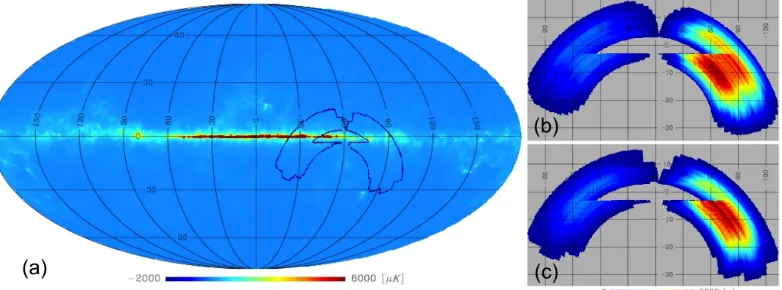
Bicep _{observed two fields over the Galactic plane as shown in Figure 1. For each field, a telescope scans}

back-and-forth in azimuth at 2.8◦/s over a 65◦ range at a constant elevation. The elevation is stepped by 0.25◦ after 50 right and left ”half-scans” at a constant elevation. The telescope observed with four different orientations about its boresight: 0◦,135◦,180◦,and 315◦. Each observation of the single field has a fixed boresight angle and four observations cover all the boresight angles to increase the crosslinking coverage.

2.1 Map making

Figures 2 shows theQandU maps observed byBicepat 100 and 150 GHz. This section describes polarized map making, focusing on processes unique to the Galactic field analysis. The map making process that is common to the CMB analysis is described in Chiang et al.8

The low-level time stream cleaning is applied to the raw time stream in following steps, (i) deconvolution of a bolometer transfer function, (ii) low-pass filtering at 5 Hz, and (iii) downsampling to 10 Hz. Thejth _sample

in a half-scan of a gain adjusted pair-differenced time stream is

di(tj) =

1 2(

di_A(tj)

gi_A −

di_B(tj)

gi_B

Figure 1. (a) The twoBicep_{Galactic regions are indicated over the FDS model 8 at 150 GHz.}28 _{Right: The integration}

time per nside=256 ofHealpixpixel at 100 GHz (b) and 150 GHz (c).29

Figure 2. TheQandU maps of the Galactic fields are shown in the unit ofμK_cmb. QandU are defined in the Galactic coordinate with IAU convention.

wheredi_A,B are the individual low-level processed time streams of ith PSB pair, andg_iA,B are the gain factors

for each PSB calibrated at every elevation step. Common mode noise between the PSB pair, such as thermal fluctuations of the instrument and atmospheric fluctuations, is removed by differencing between the two PSB pair time streams, and we fit a third order polynomial,Fi(tj), to the pair-differenced time stream in order to

remove residual 1/f noise below∼0.1 Hz.

the samples in the half-scan.

In some cases one end of the half-scan lies inside of the Galactic mask. We did not include such half-scan in the map making because the polynomial inside of the mask needs to be extrapolated from the edge of the mask and the extrapolated polynomial does not represent the 1/f noise inside of the mask. The half-scans whose two ends lie in the mask are also excluded. Consequently, the recovered maps become “pac-man” shaped. The recovered region shrinks as the mask width increases.

We follow the formalism described by Jones et al.30 and used for theBicepCMB analysis described in Chiang et al.8 TheQandU values of the pixel in the direction on the skypare computed fromd_ij =di(tj)−Fi(tj) as

Q(p)

U(p)

=M

N_{P SB}

i

j⊂p

wij

d_ijα d_ijβ

, (2)

where

M−1= 1 2

NP SB

i

j⊂p

wij

α2_ij αijβij

αijβij β2ij

(3)

and

αij =γi_Acos 2ψi_Aj−γi_Bcos 2ψi_Bj (4)

βij =γiAsin 2ψiAj−γiBsin 2ψiBj. (5)

The weightwij is an inverse of a variance ofdij calculated from the samples outside of the mask in each half-scan.

The angleψis the PSB orientations projected on the sky andγ=1−₁₊ is the polarization efficiency factor, where

is a cross-polarization response. Subscriptsi_Aandi_Brefers to the AandB bolometers of theith pair. We use nside=256 ofHealpixpixelization to projectQandU on the sky.29

2.2 Pixel noise in the map

Statistical errors in theBicep maps are estimated using jackknife maps. We split the data into three pairs of halves, (i) right and left half-scans, (ii) (0◦,315◦) and (135◦,180◦) boresight angles, (iii) two sets of detector pairs located in alternating sectors of the 6-sector circular focal plane. We compute theQandU maps of each data set as (mQ₁, mU₁) and (mQ₂, mU₂). We compute the difference as

δmQ =

1

2(mQ1−mQ2)

√

N , δmU =

1

2(mU1−mU2)

√

N , (6)

whereN is the number of observations at eachHealpixpixel. We compute the histogram ofN EQ=δmQ/

√

2fs

and N EU =δmU/

√

2fs (where fs = 10 Hz sampling rate) from the map pixels that meet the criteria of (1)

N >2000, (2) the Galactic latitude|θglat|<3◦ and (3) not being at the edge of the observed regions. (Hereafter

we call the region of the sky that meets these criteria aselectedregion.) We fit the histogram with a Gaussian

Aexp−(δm₂−_σ2m¯)2

0 .

Figure 3 shows the histograms of the jackknife maps. The noise property is well described by the Gaussian distribution. The averagedN EQandN EU from the three jackknives are 523 and 507μK√sfor 100 GHz, and 428 and 431μK√sfor 150 GHz, respectively. Among the three jackknives the worstN EQ is 16 % larger than the best one that is from the right and left half-scan jackknife.

2.3 Systematic error

Figure 3. The histograms ofδmQandδmUfor 100 and 150 GHz are shown for right/left (top), boresight angle (middle), and detector sets (bottom) jackknives.

Figure 4. Comparison of the filteredQ(andU) values of the simulated map against to the input unfiltered

Q(andU) values. The two linear lines are fits to the 100 GHz (blue) and 150 GHz (green) data. The red line indicates the line that has a slope of 1 with zero offset. The offsets of 100 and 150 GHzQsignals are -5.6 and -18.1, respectively.

Figure 5. The difference of the polarization angle at each pixel before and after applying the BICEP time domain filtering to the simulated maps is plotted. The points are selected from the pixels for the Galactic lat-itude of |θ| < 1 (red), |θ| < 2 and |θ| > 1 (black), |θ| < 3 and |θ| > 2 (blue). The four lines are |Δα| from Equation 9 with the cases for αin of 0.1◦, 2◦, 5◦ and 10◦.

Two calibration methods are used to measure the cross-polarization. One uses a modulated linearly polarized broadband noise source mounted 200 m away from the Bicep telescope. Bicep observed the source by raster scans with 18 different boresight rotation angles. The other method uses a rotating wire grid mounted at the cryostat window. The signal is generated by chopping between an ambient absorber and the sky. The cross-polarization response is measured to within±0.01.

The PSB orientation is measured with a rotating dielectric sheet mounted in front of the cryostat window in addition to the two methods described to measure the cross-polarization. The measurements were repeated through each observing year and the uncertainty of the individual PSB orientation is 0.1◦rms. After the cryostat was opened between 2006 and 2007 observing years, the PSB orientation measurements showed an average of 1◦ rotation in the absolute polarization angle. Thus, the absolute PSB orientation uncertainty is assigned to be less than 0.7◦ rms for three years of the observation periods. The detailed discussion of the polarization calibration of theBicep polarimeter is described in Takahashi et al.31

2.4 Effects due to time domain filtering

In order to quantify the amount of the time domain filtering of the Galactic signal, we prepare a simulated polarization map (Healpix pixelization of nside=256) that consists of the sum of CMB and FDS maps at 100 and 150 GHz with a beam size of 0.93◦and 0.60◦, respectively.28 The CMB map is generated bysynfastusing the cosmological parameters of the standard ΛCDM model presented in Komatsu et al.20, 29 TheQpolarization of the FDS map is made based on the relationships ofQ/T =c₀(T /Tmax)c1 observed byBicep.32 We have used

(c₀, c₁) = (0.007,−0.47) and (0.017,−0.29) for 100 and 150 GHz, respectively.

According to this polarization model, the GalacticQdepends on temperature signal. The FDS model 8 does not have the same level of the emission as it is observed by the BICEP. In order to simulate the realistic level of the Galactic emission we use the temperatureT =βTF DS, where β = 1.30 and 0.87 for 100 and 150 GHz,

respectively. TheU polarization of the FDS is set to be zero for all the pixels. The simulated maps are smoothed to the beam size of 0.93◦and 0.60◦ for 100 and 150 GHz, respectively.

We generate time ordered data using these simulated maps with the BICEP pointing and apply the same map making as we apply to the real data. Figure 4 shows the correlation between the input and filtered Q

andU for the pixels inside of the selected sky region. The relationship ofQbefore and after applying the time domain filtering is well described by a simple linear relationship. The offset generally depends on the amount of the signal contained at the Galactic plane and the offset is higher when the Galactic signal is higher. This is because the signal level at the mask boundary is significant as compared to the 1/f noise, and therefore the interpolated polynomial inside of the mask follows the trend of the Galactic signal instead of the trend from the 1/f noise. On the other hand, theU polarization does not show any clear trend. This is becauseU polarization do not contain any Galactic signal but only the polarization of the CMB. Therefore, there is no characteristic signal increase at the Galactic plane.

Figure 5 shows the change of the polarization angle after time domain filtering. The change of the polarization angle|Δα|is modeled as

Qf ilt = Qin−Q0 (7)

Uf ilt = Uin (8)

Δα = 1

2(arctan

Uf ilt

Qf ilt −

arctanUin

Qin

)

= 1

2(arctan

Ipsin 2αin

Ipcos 2αin−Q0

−αin), (9)

where Qin=Ipcos 2αin, Uin =Ipsin 2αin and Ip =

Q2_in+U_in2. Q₀ is the offset to account for the filtering effect. The time domain filtering effect to the polarization angle ranges from 0.1 to 100 degrees. Therefore, when the offset angle between theBicepmap and the map from other experiment is cross-calibrated it is important to apply the same time domain filtering to the other map.

3. ESTIMATION OF THE OFFSET ANGLE AND ITS ERROR

We describe a method to detect the overall polarization angle offset between the two polarization maps. We have two sets ofQandU maps. Ones are the Bicepmaps as the calibrated maps. The others are maps to be calibrated. In the case of comparing the maps from two different experiments, they do not necessarily have the same beam sizes, and therefore we need to deconvolve the original beam and smooth the two maps to the same beam size. The choice of the beam smoothing varies depending on the beam sizes ofBicepand other experiment to be calibrated. In this section we assume that the two sets of maps have a same beam size and are pixelized such that the noise among pixels are not correlated. We discuss the treatment of the different beam size between the separate experiments as a case-by-case basis in Section 4.

We write the second and third components of the Stokes parameter ofith pixel in the two sets of maps as

Bicep_{map : (QiB}±_{δQiB, UiB}±_{δUiB), (10)}

Uncalibrated map : (Qi±δQi, Ui±δUi), (11)

We relateQandU of the same pixel on the sky between two experiments by two parameters, offset angleδα

and the ratio of the polarized amplitudesρas

Qi

Ui

=ρi

cos 2δαi sin 2δαi

−sin 2δαi cos 2δαi

QBi

UBi

. (12)

We can solve Equation 12 forρi andαi as,

ρicos 2δαi

ρisin 2δαi

= 1

Q2_Bi+U_Bi2

QBi UBi

UBi −QBi

Qi

Ui

, (13)

and thus

δαi =

1 2arctan

UBiQi−QBiUi

QBiQi+UBiUi

= αBi−αi, (14)

ρi =

Q2_i +U_i2

Q2_Bi+U_Bi2 , (15)

whereαBi= 1₂arctanUBi/QBiandαi= 1₂arctanUi/Qi. When theQandU maps from two separate experiments

are identical,αi = 0 andρi= 1.

While the polarization calibration can be done in terms ofQandU, we expressQandU of two maps in terms of δαand ρ. This choice was made to mitigate the effect due to the spectral dependence of the instrumental bandpass location and shape mismatch between the two separate experiments.We discuss the spectral dependence of the polarization angle in Section 5.

When the QandU maps contain only signals, we have a perfect knowledge of the offset angle δαfor every pixel. When the noise is present in the maps, the noise in the map has to be propagated to an error in the offset angle. The error of the offset angle in each pixeliis

σ2δα_i (

∂δαi

∂QBi

)2σQ2_Bi+ (

∂δαi

∂UBi

)2σ2U_Bi+

∂δαi

∂QBi

∂δαi

∂UBi

σ2QU_Bi+ (

∂δαi

∂Qi

)2σQ2_i+ (

∂δαi

∂Ui

)2σU2_i+

∂δαi

∂Qi

∂δαi

∂Ui

σ2QU_i, (16)

where σQ_Bi, σU_Bi, σQU_Bi, σQ_i, σU_i, σQU_i are the pixel noise associated with QBi and UBi, and Qi and Ui,

respectively. The derivative terms are

∂δαi

∂QBi

=−1 2

UBi

Q2_Bi+U_Bi2 ,

∂δαi

∂UBi

=1 2

QBi

Q2_Bi+U_Bi2 (17) ∂δαi

∂Qi

=1 2

Ui

Q2_i +U_i2,

∂δα ∂Ui

=−1 2

Qi

Q2_i +U_i2. (18)

The derivative terms are inversely proportional to the square of the polarized intensity. This indicates that the error of the offset angle is smaller when the polarized intensity is stronger. Figure 6 shows the angle uncertainty as a function of the pixel noise inQandU maps and the polarized intensity, Q2+U2.

While a polarization angleαi varies from −90 to 90 degrees based on the signal and the pixel noise at the

given point on the sky, we assume that the distribution of the differenced angleδαi is a Gaussian. We validate

this assumption in Section 4 when we apply this formalism betweenBicep _andWmap_.

The Galaxy is not a single point source, and therefore the estimation of the polarization offset angle improves by including all the available pixels in the map. In order to calculate the mean polarization offset angle,δα₀, between the reference and the uncalibrated polarimeter maps and the corresponding uncertainty of the mean, we compute the likelihood ofδα₀as

L∝e−12χ2(δα0)_{, (19)}

where

χ2(δα₀) =

i

(δαi−δα0)2

σ_δα2

i

Figure 6. This plot shows the angle uncertainty of the polarization signal at a given pixel as a function of a pixel noise and a polarized intensity of the signal. For an example, a map that has a pixel noise of 10μKand polarized intensity of 100μK has a polarization angle error of 3◦.

Figure 7. The spectra of BICEP (red) and WMAP W band (black). Both spectra are normalized to the maximum value of 1. The BICEP spectrum is the aver-age of a PSB pair. The WMAP spectrum is the averaver-age of the W band spectra.

4. RESULTS

We apply the method described in the previous section toBicep and Wmap. We also compute the expected constraint toPlanckandEPIC, by using BICEP Galactic map.

4.1 Polarization angle offset between

Bicep

and

Wmap

Wmap has been observing the temperature and polarization over the full sky.33 The spectral bandwidth of Bicep _{100 GHz and the} Wmap _{W band overlap as shown in Figure 7. In this exercise, we assume that the}

absolute polarization angle of theWmap_{polarimeter is unknown and we constrain the overall offset angle of the} Wmap_{polarization maps using the}Bicep _{Galactic map as a polarization calibration source.}

Before we apply the formalism described in Section 3, we need to correct the beam size difference between the two experiments. The FWHM of theBicepbeam size at 100 GHz is 0.93◦. Each of theQandU maps of the fourWmapW band differencing assembly is deconvolved with the correspondingWmapB_land convolved with FWHM of 0.93◦ Gaussian beam in nside=512 pixelization. We compute the weighted averaged map from the four differencing assembly maps in W band. The weights are the inverse of the pixel variance of each differencing assembly. We apply theBicep _{time domain filtering to the averaged}Wmap_{W band map. The filtered Qand}

U maps are downsampled to 0.92◦ pixel size (nside=64) maps in order to decorrelate the noise among pixels. TheBicep _{QandU maps are also downsampled to the same pixelization.}

The pixel noise of theWmapmaps is computed byσ=√σ0

N_hits whereσ0 for theWmapW band differencing

assemblies is (σW₁, σW₂, σW₃, σW₄) = (5.940,6.612,6.983,6.840) mK with nside=512 pixelization. We neglect the

correlated noise betweenQand U for both experiments. The pixel noise of theBicep _{maps is computed based} on theN EQ(U) derived from the right and left jackknife maps.

Once the two sets of the maps and weights are computed in the same pixelization, we impose the criteria to select the pixels. We choose the pixels that meet the criteria of|θglat|<3◦,Nhits ofBicep >2000 and pixels of which its neighbor do not have Nhits = 0. The second criterion assures that the most of the edge pixels of

the map are not included. The second criterion does not exclude the pixel around 282◦ < φglon < 322◦ and

|θglat| < 3◦ where the edge of the map is not tapered by Nhits. Therefore, we include the third criterion to

exclude all the edge pixels in the maps.

Figure 8 shows the map of offset angle δαi and the weight 1/σ2δα_i. It is clear that the the offset angle is

Figure 8. The maps of δα_i (left) in unit of degrees and weight = 1/σ_δα2 _i (right) in unit of degree−2. The maps are downsampled toHealpix resolution of nside=64. The edge pixels are removed, and therefore the shape of the map does not coincide with the ones in Figure 2.

Figure 9. The weighted histogram ofδα between the polarization maps ofBicepandWmapand the

Gaus-sian fit are shown. The distribution is well described as a Gaussian.

Figure 10. The likelihood of δα(solid black) with the pixel noise estimated from the right and left jackknife and δα(dash black) with the pixel noise increased by 16 % as a worst pixel noise estimation. The histogram is a mean of the Gaussian fit toδαfrom the two sets of the simulated signal (CMB+FDS) at 100 GHz and the 300 noise realizations. The red curve is the Gaussian fit to the histogram.

mean and the standard deviation of the angle uncertainty of each pixel is−0.41◦ and 11.2◦, respectively. The distribution of the histogram is well described as a Gaussian distribution.

Figure 10 shows the likelihood of the offset angle calculated based on Equation 19 using theBicep and the filteredWmapmaps. The black line shows that the mean and the sigma are the 0.6◦ and 1.4◦respectively. The dashed line with the same mean has 16% larger sigma as a worst case pixel noise.

The histogram in Figure 10 is the results of the signal and noise simulations. We prepare two sets of maps by adding the white noise of theBicep_{100 GHz and}Wmap_{W band to the simulated signal only maps at 100 GHz} described in Section 2.4. We repeat computing the mean of the Gaussian fit to the histogram ofδα from the two sets of the map for the 300 noise realization. The fit to this histogram in Figure 7 is consistent with the likelihood obtained by the using Equation 19.

4.2 Polarization offset angle between BICEP and future experiments

1σerror [◦] Reference×Uncalibrated 100 GHz 150 GHz

Bicep×No noise experiment 1.24 0.27

Bicep ×Wmap_{W-band 1.45}

Bicep×Planck 1.26 0.27

Bicep ×EPIC-IM (4K option) 1.24 0.26 (Bicep,Bicep2)×Planck 1.26 0.08 (Bicep_, Bicep2_, Keck₎×Planck _{0.23 0.06}

Table 1. The 1σ statistical error of the polarization angle offset for various combinations of the experiments. The first row,Bicep×_{No noise experiment, indicates the angle error only due to the}Bicep_{statistical noise.} Bicep2_{only has}

150 GHz band, and therefore the error in 100 GHz does not show any improvement.

for two cases,Bicep andPlanck, andBicepandEPIC.35

Table 1 shows the list of 1σstatistical error from the likelihood in Equation 19 for 100 GHz and 150 GHz for the two experiments. In this comparison, we assume that the bandpass shape of the two separate experiments is the same and the knowledge of the beam shape is perfect.

The expected pixel noise ofPlanckandEPIC-IM are fromPlanckbluebook and Bock et al., respectively.34, 35 It is clear that the estimate of the 1σerror of the offset angle betweenBicep andWmapimproves withBicep andPlanckorEPIC-IM. This is because the noise contribution fromPlanckandEPIC-IM is much smaller than the case fromWmap_{while the}Bicep _{noise stays the same. On the other hand, there is negligible improvement} fromPlanckto EPIC_{-IM because the source of the noise in these two cases is limited by the pixel noise of the} Bicep_map.

While the observations ofBicep were completed, the ongoingBicep2and forthcomingKeck will improve the sensitivity to the angle calibration. If we assume thatBicep2andKeckwill spend the same observational time with the same detector sensitivity on the BICEP Galactic field, the expected reduction of the pixel noise is

simply scaled by NBicep

NBicep+N0, whereNBicepis the number of detectors ofBicepandN0is ofBicep2orBicep2

andKeck_{. We assume thatNBicep is 25 and 24 for 100 and 150 GHz, andN0 is 256 for}Bicep2_{150 GHz and} 144×4 and 256×2 for 100 and 150 GHz ofKeck_{, respectively. The data combining with} Bicep2_andKeck provide the statistical errors of the offset angle smaller than the systematic errors of theBicep_{polarimeter itself} for both 100 and 150 GHz bands.

5. DISCUSSION

5.1 Comparison between the diffuse Galactic source and the Crab nebula as a polarized

calibration source

We compare the Crab nebula and the BICEP Galactic region as a polarized source. The emission mechanism of the Crab nebula at the millimeter wavelength is dominated by the synchrotron emission. Macias-Perez et al. and Weiland et al. reported that the observed flux has a power law of∝(_40GHzν )−0.3∼−0.35 while the degree of polarization stays constant around 7 % over the millimeter wavelength.24, 36 On the other hand, the diffuse dust emission at the Galactic plane increases as a function of frequency.32 Therefore, the signal-to-noise increases as the bandpass location increases.

Band Q[Jy] U [Jy] Angle [◦] WMAP, Crab nebula

K band −27.13±0.68 −1.40±0.08 −88.5±0.1 Ka band −23.72±0.45 −1.88±0.12 −87.7±0.1 Q band −22.03±0.60 −2.06±0.14 −87.3±0.2 V band −19.25±0.36 −1.52±0.24 −87.7±0.4 W band −16.58±0.73 −0.75±0.42 −88.7±0.7

all band combined 0.07

Aumont et al., Crab nebula

90 GHz −88.8±0.2

BICEP Galaxy

100 GHz 114.7±6.0 29.1±6.2 ±1.5 150 GHz 573.4±12.2 195.6±11.2 ±0.5

Table 2. The integrated polarized flux of the Crab nebula and the Bicep_{Galactic region is shown. The polarization}

convention in this paper and Wmap_{are different, and thus the sign of} U _{is changed from the original WMAP paper.}

The angle error of theBicepGalactic measurements is the quadrature sum of the pixel noise. †The polarization angle

seen by 10 beam from Aumont et al. The original literature quoted the polarization angle in equatorial coordinates as

α= 148.8◦.

5.2 Effect of spectral mismatch between two experiments

When the two polarization maps from two separate experiments are cross-calibrated, the spectral bandpass of the two experiments is not necessary the same. We assess the effect of the bandpass mismatch to the offset angle estimation between theBicep 100 GHz band and theWmapW band.

Gold et al. derived the synchrotron and dust emission templates by the Markov chain Monte Carlo fitting.37 We compute the simulatedBicepandWmapmaps by integrating the sum of the synchrotron and dust template maps over theBicep100 GHz bandpass andWmapW band bandpass. We compute the offset angleδα_i of each pixel between the two bandpass maps. The median offset angle of all the pixels within the selected sky region is 0.005◦. We define the signal-to-noise for each pixel as the ratio of the polarized intensity to the pixel noise. We compute the median and the maximum offset angle of which the pixels are the signal-to-noise>3 are 0.01◦and 0.02◦, respectively.

The Bicep 100 GHz map expects a higher contribution of the dust emission as compared to the Wmap W band map because theBicep100 GHz bandwidth is slightly wider thanWmapW band bandwidth in higher frequency side as shown in Figure 7. Gold et al. shows that in theBicepGalactic field the polarization direction of the synchrotron emission is−26◦< αsynch<0◦ and that of the dust emission is |αdust|<0.3◦. Therefore,

the overall offset angle between theBicep and Wmap maps is expected to show the positive rotation due to the bandpass mismatch. The overall offset angle between theBicep and Wmapmaps, shown in Figure 7 , is 0.6◦±1.4◦, and the positive mean value is consistent with the bandpass mismatch.

This effect is prominent when the passband of the instrument is located where more than two emission spectra are mixed with nearly the same amplitude. This is because the two sources with different spectral shape can have different polarization angles.

6. CONCLUSION

We present the polarized diffuse Galactic emissions observed byBicep _{at 100 and 150 GHz and the method to} cross-calibrate the absolute angle between theBicepmap and any uncalibrated map. The absolute angle of the Biceppolarimeter is calibrated to±0.7◦ and the 1σerror of the polarization angle due to the pixel noise of the Bicepmap is 1.24◦ and 0.27◦for 100 and 150 GHz, respectively.

TheBicep _{Galactic maps provide the polarized Galactic emission as a new angle calibration source for the} ongoing and forthcoming CMB B-mode experiments that require the absolute angle calibration to a fraction of a degree. The method of using the Galactic signal as an angle calibration source can be applied to any two experiments if one of the polarimeters is well calibrated. Therefore, when thePlanckfull sky polarization maps are available, the future polarimeters should be able to use the Galactic signal as a calibration source not only with respect toBicepbut also toPlanck.

REFERENCES

[1] W. Hu and M. White, A CMB polarization primer, New Astronomy, 2, pp. 323-344, 1997.

[2] J. M. Kovac 2002, Detection of polarization in the cosmic microwave background using DASI, Nature, 420, 772, astro-ph/0209478.

[3] T. Montroy et al. 2006 ApJ 647 813.

[4] Sievers et al., The Astrophysical Journal, 660:976 987, 2007 May 10. [5] J. H. P. Wu et al. 2007 ApJ 665 55.

[6] M. L. Brown et al. 2009 ApJ 705 978. [7] L. Page, et al., 2007, ApJS, 170, 335. [8] H. C. Chiang et al. 2010 ApJ 711 1123. [9] L. Pagano et al., Phys. Rev. D80:043522,2009.

[10] Reichborn-Kjennerud et al. Submitted to these proceedings. [11] Ogburn et al., Submitted to these proceedings.

[12] Sheehy et al., Submitted to these proceedings. [13] Arnold et al., Submitted to these proceedings.

[14] D. Samtleben et al., In the Proceedings ‘A Century of Cosmology’, San Servolo (Venezia, Italy), August 2007. arXiv:astro-ph/0802.2657.

[15] Crill et al. Proceedings of SPIE Volume 7010. arXiv:0807.1548v1. [16] Filippini et al. Submitted to these proceedings.

[17] Weiss et al. Task Force on Cosmic Microwave Background Research,’ arXiv:astro-ph/0604101v1. [18] J. Q. Xia et al., Phys. Lett. B687:129-132,2010.

[19] Wu et al. QUaD Collaboration. Phys. Rev. Lett. 102, 161302 (2009).

[20] Komatsu et al. Seven-Year Wilkinson Microwave Anisotropy Probe (WMAP) Observations. Submitted to ApJ. http://lambda.gsfc.nasa.gov/

[21] Aumont et al. A&A 514, A70 (2010). [22] Zemcov et al. 2010 ApJ. 710 1541. [23] Leitch et al., Nature 420 (2002) 763-771.

[24] Weiland et al. Seven-Year Wilkinson Microwave Anisotropy Probe (WMAP) Observations. Submitted to ApJ. http://lambda.gsfc.nasa.gov/

[25] Tauber et al., The Extragalactic Infrared Background and its Cosmological Implications. IAU Symposium, vol. 204 2001.

[26] Rosset, C. et al., ”” Accepted by Astronomy&Astrophysics, April 12, (2010). [27] Yoon, K. W., et al. 2006, Proceedings of SPIE Volume 6275,

[28] Finkbeiner, D. P., Davis, M., & Schlegel, D. J. 1999, Astrophys. J. , 524, 867, astro-ph/9905128. [29] Gorski, K.M. et al., 2005, Astrophys. J., 622,759.

[30] W. C. Jones et al., Astr. & Astroph. , 470, Issue 2, 771785, August 2007, astro-ph/0606606. [31] Y. D. Takahashi et al. 2010 ApJ 711 1141.

[32] Bierman et al. Submitted to these proceedings.

[33] Jarosik et al. Seven-Year Wilkinson Microwave Anisotropy Probe (WMAP) Observations. Submitted to ApJ. http://lambda.gsfc.nasa.gov/

[34] Planck bluebook. ESA-SCI(2005)1. http://www.rssd.esa.int/Planck/

[35] J. Bock et al. Study of the Experimental Probe of Inflationary Cosmology (EPIC)-Intemediate Mission for NASA’s Einstein Inflation Probe. arXiv:0906.1188v1.

[36] Marcias-Perez et al., ApJ. 711:417-423, 2010 March 1.