Introducing Expected Returns into Risk Parity Portfolios: A New Framework for Tactical and Strategic Asset Allocation

Introducing Expected Returns into Risk

Parity Portfolios: A New Framework for

Tactical and Strategic Asset Allocation

Roncalli, Thierry

Lyxor Asset Management University of Evry

1 July 2013

Online at

https://mpra.ub.uni-muenchen.de/49821/

Parity Portfolios: A New Framework for

Tactical and Strategic Asset Allocation

∗

Thierry Roncalli

Research & Development

Lyxor Asset Management, Paris

thierry.roncalli@lyxor.com

July 2013

Abstract

Risk parity is an allocation method used to build diversified portfolios that does not rely on any assumptions of expected returns, thus placing risk management at the heart of the strategy. This explains why risk parity became a popular investment model after the global financial crisis in 2008. However, risk parity has also been criticized because it focuses on managing risk concentration rather than portfolio performance, and is therefore seen as being closer to passive management than active management. In this article, we show how to introduce assumptions of expected returns into risk parity portfolios. To do this, we consider a generalized risk measure that takes into account both the portfolio return and volatility. However, the trade-off between performance and volatility contributions creates some difficulty, while the risk budgeting problem must be clearly defined. After deriving the theoretical properties of such risk budgeting portfolios, we apply this new model to asset allocation. First, we consider long-term investment policy and the determination of strategic asset allocation. We then consider dynamic allocation and show how to build risk parity funds that depend on expected returns.

Keywords: Risk parity, risk budgeting, expected returns, ERC portfolio, value-at-risk, expected shortfall, tactical asset allocation, strategic asset allocation.

JEL classification: G11.

1

Introduction

Although portfolio management didn’t change much in the 40 years following the seminal works of Markowitz and Sharpe, the development of risk budgeting techniques marked an important milestone in the deepening of the relationship between risk and asset management. Risk parity subsequently became a popular financial model of investment after the global financial crisis in 2008. Today, pension funds and institutional investors are using this approach in the development of smart beta and the redefinition of long-term investment policies (Roncalli, 2013).

∗_{I would like to thank Lionel Martellini, Vincent Milhau and Guillaume Weisang for their helpful}

In a risk budgeting (RB) portfolio, the ex-ante risk contributions are equal to some given risk budgets. Generally, the allocation is carried out by taking into account a volatility risk measure. It simplifies the computation, especially when a large number of assets is involved. However, the volatility risk measure has been criticized because it assumes that asset re-turns are normally distributed (Boudtet al., 2013). There are now different approaches to extending the risk budgeting method by considering non-normal asset returns. However, in our view, these extensions do not generally produce better results. Moreover, we face some computational problems when implementing them for large asset universes.

A more interesting extension is the introduction of expected returns into the risk bud-geting approach. Risk parity is generally presented as an allocation method unrelated to the Markowitz approach. Most of the time, these are opposed, because risk parity does not depend on expected returns. This is the strength of such an approach. In particular, with an equal risk contribution (ERC) portfolio, the risk budgets are the same for all assets (Maillardet al., 2010). This may be interpreted as the neutral portfolio when the portfolio manager has no views. However, the risk parity approach has also been strongly criticized, because some investment professionals consider this aspect a weakness. Some active man-agers have subsequently reintroduced expected returns in an ad hoc manner. For instance, they modify the weights of the risk parity portfolio in a second step by applying the Black-Litterman model or optimizing the tracking error. A second solution consists of linking the risk budgets to the expected returns. In this paper, we propose another route. We con-sider a generalized standard deviation-based risk measure, which encompasses the Gaussian value-at-risk and expected shortfall risk measures. We often forget that these risk measures depend on the vector of expected returns. In this case, the risk contribution of an asset has two components: a performance contribution and a volatility contribution. A positive view on one asset will reduce its risk contribution and increase its allocation. But, contrary to the mean-variance framework, the RB portfolio obtained remains relatively diversified.

The introduction of expected returns into risk parity portfolios is particulary relevant in a strategic asset allocation (SAA). SAA is the main component of long-term investment policy. It concerns the portfolio of equities, bonds and alternative assets that the investor wishes to hold over the long run (typically 10 years to 30 years). Risk parity portfolios based on the volatility risk measure define well-diversified strategic portfolios. The use of a standard deviation-based risk measure allows the risk premia of the different asset classes to be taken into account. Risk parity may also be relevant in a tactical asset allocation (TAA). In this case, it may be viewed as an alternative method to the Black-Litterman model. Active managers may then naturally incorporate their bets into the RB portfolio, and continue to benefit from the diversification. This framework has been already used by Martellini and Milhau (2013) to understand the behavior of risk parity funds with respect to economic environments. In particular, they show how to improve the risk parity strategy in the context of rises in interest rates.

2

The framework

2.1

Combining performance allocation and risk allocation

We consider a universe ofnrisky assets1_{. Letµand Σ be the vector of expected returns and}

the covariance matrix of asset returns. We have Σi,j=ρi,jσiσj whereσi is the volatility of

assetiandρi,jis the correlation between assetiand assetj. The mean-variance optimization

(MVO) model is the traditional method for optimizing performance and risk (Markowitz, 1952). This is generally done by considering the following quadratic programming problem:

x⋆_{(γ) = arg min}1

2x

⊤_Σx

−γx⊤_(µ

−r1)

where x is the vector of portfolio weights, γ is a parameter to control the investor’s risk aversion and r is the return of the risk-free asset. Sometimes restrictions are imposed to reflect the constraints of the investor. For instance, we impose that 1⊤_{x = 1 and x ≥0}

for a long-only portfolio. This framework is particularly appealing because the objective function has a concrete financial interpretation in terms of utility functions. Indeed, the investor faces a trade-off between risk and performance. To obtain a better expected return, the investor must then choose a portfolio with a higher risk.

Remark 1 Without loss of generality, we require thatris equal to0. All the results obtained in this article may then be generalized by replacing the vector of expected returnsµwith the vector of risk premiaπ=µ₋r.

However, the mean-variance framework has been hotly debated for some time (Michaud, 1989). The stability of the MVO allocation is an open issue, even if some methods can regularize the optimized portfolio (Bruderet al., 2013). The problem is that the Markowitz optimization is a very aggressive model of active management (Roncalli, 2013). It detects arbitrage opportunities that are sometimes false and may result from noise data. The model then transforms these arbitrage opportunities into investment bets in an optimistic way without considering adverse scenarios. This problem is particularly relevant when the input parameters are historical estimates. In this case, the Markowitz optimization is equivalent to optimizing the in-the-sample backtest.

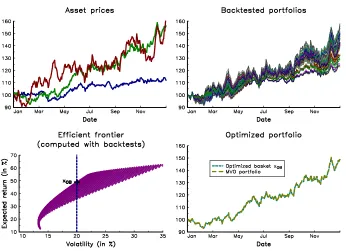
We consider three assets whose asset pricesPi,t are given in the first panel in Figure 1.

We simulate the performance of the basket (x1, x2, x3) by assuming that the initial wealth

is equal to 100 dollars:

St= 100·

x1P1,t+x2P2,t+x3P3,t

x1P1,0+x2P2,0+x3P3,0

In the second panel, we report the performance of different simulated long-only portfolios. We can then define the empirical efficient frontier by computing the return and the volatility for a large number of simulated portfolios. If we suppose that we are targeting a volatility equal to 20%, we obtain the optimized basketxOBlocated in the empirical efficient frontier.

In the last panel, we compare the performance of this portfolio, which was determined solely by the in-the-sample backtesting, and the performance of the MVO portfolio, which was estimated on the basis of the empirical mean and covariance matrix of the asset returns. We obtained exactly the same result. We then verified that the MVO portfolio corresponds to the portfolio that maximizes the backtest performance when we consider historical estimates.

1

Figure 1: In-the-sample backtesting and the Markowitz solution

Despite the previous drawback, the Markowitz model remains an excellent tool for com-bining performance allocation and risk allocation. Moreover, as noted by Roncalli (2013), “there are no other serious and powerful models to take into account return forecasts”. The only other model that is extensively used in active management is the Black-Litterman model, but it may be viewed as an extension of the Markowitz model. In both cases, the trade-off between return and risk is highlighted. Let µ(x) = x⊤_{µ and σ(x) =} √_x⊤_Σx

be the expected return and the volatility of portfoliox. The Markowitz model consists of maximizing the quadratic utility function:

U(x) =µ(x)−φ₂σ2(x)

where φ = γ−1 _{is the risk aversion with respect to the variance. It is obvious that the}

optimization problem can also be formulated as follows:

x⋆_{(c) = arg min}

−µ(x) +c_·σ(x)

The mapping between the solutionsx⋆_{(γ) andx}⋆_{(c) is given by the relationship:}

c= 1 2γσ(x

⋆_(γ))

In terms of risk aversion, we obtain:

φ= 1 γ =

2c σ(x⋆_(γ))

Example 1 We consider four assets. Their expected returns are equal to5%,6%,8%and

of asset returns is given by the following matrix:

C=

   

1.00 0.10 1.00 0.40 0.70 1.00 0.50 0.40 0.80 1.00

   

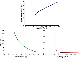
In Figure 2, we report the efficient frontier of optimized portfolios using Example 1. We also represent the relationships betweenσ(x⋆_{(γ)) and the ratioφ/cand betweenσ(x}⋆_(γ))

andc. We have verified that the scalarc is a decreasing function of the optimized volatil-ity. However, we also noticed that the discrepancy in terms ofc is very low for optimized portfolios that are not close to the minimum variance portfolio.

Figure 2: Relationship between MVO portfolios and the scaling factorc

Remark 2 We can interpret the Markowitz optimization problem as a risk minimization problem:

x⋆_{(c) = arg min}

R(x)

whereR(x)is the risk measure defined as follows:

R(x) =−µ(x) +c·σ(x)

It is remarkable to note that the Markowitz model is therefore equivalent to minimizing a risk measure that encompasses both the performance dimension and the risk dimension.

2.2

Interpretation of the Markowitz risk measure

haveL(x) =₋x⊤_{R whereR is the random vector of returns. We consider the generalized}

standard deviation-based risk measure:

R(x) = E[L(x)] +c_·σ(L(x)) = −µ(x) +c·σ(x)

If we assume that the asset returns are normally distributed:R∼ N(µ,Σ), we haveµ(x) = x⊤_{µandσ(x) =}√_x⊤_{Σx. It follows that:}

R(x) =₋x⊤_µ+c

·√x⊤_Σx

We obtain the Markowitz risk measure. This formulation encompasses two well-known risk measures (Roncalli, 2013):

• Gaussian value-at-risk:

VaRα(x) =−x⊤µ+ Φ−1(α)

√

x⊤_Σx

In this case, the scaling factorc is equal to Φ−1_(α).

• Gaussian expected shortfall:

ESα(x) =−x⊤µ+

√

x⊤_Σx

(1−α)φ Φ

−1_(α)

Like the value-at-risk measure, it is a standard deviation-based risk measure where the scaling factorc is equal toφ Φ−1_(α)

/(1₋α).

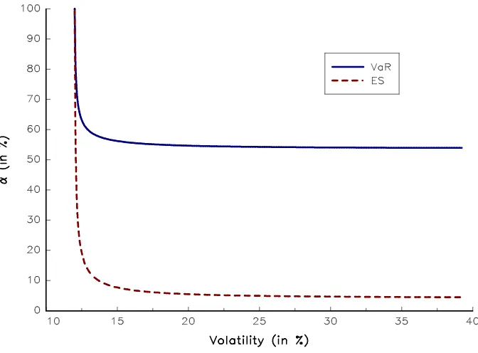
Let us consider Example 1 again. In Figure 3, we show the relationship between mean-variance optimized portfolios and the confidence levelαof the value-at-risk and expected shortfall risk measures2_.

We deduce that the expression of the marginal risk is:

MRi=−µi+c

(Σx)i

√

x⊤_Σx

It follows that:

RCi = xi·

−µi+c

(Σx)_i

√

x⊤_Σx

= ₋xiµi+c

xi·(Σx)i

√

x⊤_Σx

We verify that the standard deviation-based risk measure satisfies the Euler decomposition (Roncalli, 2013):

R(x) =

n

X

i=1

RCi

2

For the value-at-risk, we have:

α= Φ

_σ(x⋆

(γ)) 2γ

whereas the confidence levelαsatisfies the following non-linear equation for the expected-shortfall:

φ Φ−1

(α)+ασ(x

⋆

(γ)) 2γ −

σ(x⋆

Figure 3: Relationship between MVO portfolios and the confidence levelα

This implies that it is a good candidate for a risk budgeting approach.

In Table 1, we consider Example 1 and report the risk decomposition of the equally weighted (EW) portfolio by taking into account the volatility risk measure3_{. For each asset,}

we give the weightxi, the marginal risk MRi, the nominal risk contribution RCi and the

relative risk contribution _RC⋆i. All the statistics are expressed in %. We notice that the

fourth asset is the main contributor because it represents 36.80% of the portfolio’s risk. If we use the value-at-risk with a confidence level equal to 99%, we obtain similar results in terms of relative risk contributions (see Table 2). This is because the expected returns are homogeneous within a range of 5% and 6%.

Table 1: Volatility decomposition of the EW portfolio

Asset xi MRi RCi RC⋆i

1 25.00 8.62 2.16 11.80

2 25.00 13.96 3.49 19.10 3 25.00 23.61 5.90 32.30 4 25.00 26.89 6.72 36.80

Volatility 18.27

Suppose now that the expected returns are−15%,−15%, 15% and 25%. This implies that the portfolio manager has a negative view of the first and second assets and a positive

3

Table 2: Value-at-risk decomposition of the EW portfolio

Asset xi MRi RCi RC⋆i

1 25.00 15.06 3.76 10.38

2 25.00 26.47 6.62 18.26

3 25.00 46.92 11.73 32.36 4 25.00 56.56 14.14 39.00

Value-at-risk 36.25

view of the third and fourth assets. These views then have an impact on the risk decom-position if the risk measure corresponds to the value-at-risk. For instance, we observe now that the main contributor is the second asset (see Table 3).

Table 3: Value-at-risk decomposition with the second set of expected returns

Asset xi MRi RCi RC⋆i

1 25.00 35.06 8.76 21.91

2 25.00 47.47 11.87 29.67

3 25.00 39.92 9.98 24.95

4 25.00 37.56 9.39 23.47

Value-at-risk 40.00

2.3

Relationship between the risk contribution, return contribution

and volatility contribution

We notice that the risk contribution has two components. The first component is the opposite of the performance contributionµi(x), while the second component corresponds

to the standard risk contributionσi(x) based on the volatility risk measure. We can then

reformulateRCi as follows:

RCi=−µi(x) +cσi(x)

withµi(x) =xiµi andσi(x) = xi·(Σx)_i/σ(x).

We define the normalized risk contribution of assetias follows:

RC⋆ i = −

µi(x) +cσi(x)

R(x)

In the same way, the normalized performance (or return) contribution is:

PC⋆ i =

µi(x)

µ(x)

= Pnxiµi

while the volatility contribution is4_:

VC⋆ i =

σi(x)

σ(x)

= xi·(Σx)i

x⊤_Σx

We then obtain the following proposition.

Proposition 1 The risk contribution of asset i is the weighted average of the return con-tribution and the volatility concon-tribution:

RC⋆

i = (1−ω)PC ⋆ i +ωVC

⋆ i

where the weightω is:

ω= cσ(x)

−µ(x) +cσ(x)

Remark 3 The range of ω is]_−∞,_∞[. If c = 0, ω is equal to 0. ω is then a decreasing function with respect toc until the valuec⋆_{=µ(x)/σ(x), which is the ex-ante Sharpe ratio}

of the portfolio5_{. If c > c}⋆_{, ω is positive and tends to one when c tends to}

∞. Figure 4 illustrates the relationship betweencandωfor different values of the Sharpe ratioSR (x|r). We conclude that the risk contribution is a return-based (or volatility-based) contribution ifc

is lower (or higher) than the Sharpe ratio of the portfolio. The singularity around the Sharpe ratio implies that the value ofc must be carefully calibrated.

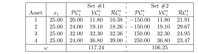
Let us consider Example 1. In Table 4, we report the return, volatility and risk contribu-tions when the risk measure is the value-at-risk with a 99% confidence level. If we consider the original expected returns (Set #1), the weightω is equal to 117.24%. We set out the results obtained in Table 2. If we consider the second set of expected returns (Set #2), the impact of the return contributions is higher even ifωis close to 1. The reason is that there is a considerable difference in performance contribution. For instance, the return contribution of the first asset is equal to−150%, whereas it is equal to +250% for the fourth asset.

Table 4: Return and volatility contributions

Set #1 Set #2

Asset xi PC⋆i VC ⋆ i RC ⋆ i PC ⋆ i VC ⋆ i RC ⋆ i

1 25.00 20.00 11.80 10.38 ₋150.00 11.80 21.91 2 25.00 24.00 19.10 18.26 ₋150.00 19.10 29.67 3 25.00 32.00 32.30 32.36 150.00 32.30 24.95 4 25.00 24.00 36.80 39.00 250.00 36.80 23.47

ω 117.24 106.25

4

The volatility contribution is the traditional risk contribution used in asset management (Roncalli, 2013). For instance, the ERC portfolio defined by Maillardet al. _{(2010) is based on this statistic.}

5

If the risk-free rate is not equal to zero, the risk measure isR(x) =−(µ(x)−r) +c·σ(x). We then haveRCi=−xi(µi−r) +c xi·(Σx)i

σ(x). In this case,c⋆

takes the following value:

c⋆

= µ(x)−r

Figure 4: Weightω of the volatility contribution

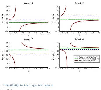
We suppose now that the expected returns are 8%, 12%, 10% and 15%. In Figure 5, we report the evolution of the return, volatility and risk contributions (in %) with respect toc. We thus verified that the risk contribution is not a monotone and a continuous function of c. We can easily understand this result because the risk measure is an increasing function of the portfolio’s volatility, but a negative function of the portfolio’s return. However, it is a serious drawback, especially when we consider risk budgeting portfolios in a dynamic framework. This is why we generally require that the coefficientcis larger than the ex-ante Sharpe ratio in order to use volatility-based risk contributions.

2.4

Sensitivity analysis of risk contributions

In this paragraph, we suppose that the scaling factorc is larger than a boundc⋆ _{that we}

will specify later.

2.4.1 Sensitivity to the scaling factor

We have:

RC⋆ i =PC

⋆

i +ω(VC ⋆ i − PC

⋆ i)

We deduce that:

∂_RC⋆ i

∂ c = (VC

⋆ i − PC

⋆ i)

∂ ω ∂ c

It follows that the normalized risk contribution of assetiis a decreasing function ofc if the volatility contribution_VC⋆

i is larger than the return contribution PC ⋆

i. This effect has been

Figure 5: Change in the contributions with respect toc

2.4.2 Sensitivity to the expected return

We notice that:

∂_RC⋆ i

∂ µi

= xi(RCi− R(x))

R2_(x)

and:

∂RC⋆ i

∂ µj

= xiRCj

R2_(x)

Remember that_R(x) is a convex risk measure. In this case, we may show that we (generally) haveRCi ≤ R(x) (Roncalli, 2013). It follows that:

∂_RC⋆ i

∂ µi ≤

0

The risk contribution_RC⋆i is a decreasing function of µi. The larger the expected return,

the smaller the risk contribution. The impact of µj is less straightforward. We generally

have RCj >0, meaning that RC⋆i is an increasing function of µj. However, we may find

some situations where RCj < 0 (Roncalli, 2013). For example, this is the case when the

correlations of assetj are negative on average and its weight is low.

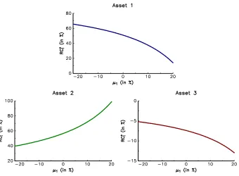
Example 2 We consider a universe of three assets. The volatilities are equal to15%,20%

and20%, while the expected returns of the second and third assets are equal to 10%and3%. The correlation matrix of asset returns is given by the following matrix:

C=

 

1.00

0.50 1.00

−0.50 −0.30 1.00

In Figure 6, we report the values taken by _RC⋆

i whenµ1 is between−20% and +20%.

We verify that the risk contribution of the first asset decreases withµ1, and we observe that

RC⋆2 is an increasing function ofµ1. This is not the case forRC⋆3, becauseRC

⋆

3 is negative.

Figure 6: Sensitivity to the expected returnµ1

2.4.3 Sensitivity to the volatility and the correlation

The parameterσi has an impact on the volatility part of the standard deviation-based risk

measure. We then achieve similar results as those obtained for the volatility risk measure. This implies that the risk contribution of assetiis generally a decreasing function of volatility σi. The behavior of the risk contribution with respect to the correlationρi,j is less obvious,

and it is highly dependent on the portfolio weights (Roncalli, 2013).

2.4.4 Sensitivity to weights

We have:

∂_RCi

∂ xi

=c 2xiσ

2

i +σiSi

σ(x) − µi+c

xi xiσ2i +σiSi

2

σ3_(x)

!

whereSi=P_j6=ixjρi,jσj. The risk contributionRCi is therefore not a monotone function

of the weightxi. Nevertheless, if the correlations are all positive, and if the expected returns

are small, the risk contribution of assetidecreases with its weight.

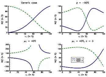
Example 3 We consider a universe of two assets. The expected return is equal to 10%

In Figure 7, we report the evolution of_RC⋆

1andRC⋆2with respect to the weightx1. The

first panel corresponds to the parameter set of Example 3. We notice that the risk contri-bution increases with the weight. Let us now change the parameter set. If the correlation is equal to₋50%, the risk contribution is an increasing function only if the weight is low or high (see panel 2). If we assume thatµ1 is equal to 40%, we observe a singular behavior.

The problem comes from the scaling factorc which is too small. For instance, ifc is equal to 3, we obtain the results given in the fourth panel.

Figure 7: Sensitivity to the weight x1

3

Risk budgeting portfolios

3.1

The right specification of the RB portfolio

Roncalli (2013) defines the RB portfolio using the following non-linear system:

          

RCi(x) =biR(x)

bi>0

xi≥0

Pn

i=1bi= 1

Pn

i=1xi= 1

(1)

where bi is the risk budget of asset i expressed in relative terms. The constraintbi > 0

implies that we cannot set some risk budgets to zero. This restriction is necessary in order to ensure that the RB portfolio is unique (Bruder and Roncalli, 2012). When using a standard deviation-based risk measure, we have to impose a second restriction:

If _{0_{} ∈} Im_R(x), it implies that the risk measure can take both positive and negative values. We then face a singularity problem, meaning that there may be no solution to the system (1). The restriction (2) is equivalent to requiring that the scaling factorc is larger than the boundc⋆ _{defined as follows:}

c⋆ _{= SR}+

= max sup

x∈[0,1]n

SR (x_|r),0

!

Remark 4 In fact, we can show that the RB portfolio is well-defined if we impose the following restriction6_:

c_∈

0,SR−

∪

SR+,_∞

(3)

with:

SR−= max

inf

x∈[0,1]nSR (x|r),0

Let us consider Example 3 withµ1 = 40%. In Figure 8, we show the evolution of the

Sharpe ratio with respect to the weightx1. The maximum (or minimum) value is reached

when the portfolio is fully invested in the first (or second) asset, and we obtain SR−= 0.50 and SR+ = 2.67. We can understand why there is no solution to the RB problem whenc is equal to 2 (see Figure 3). Because c is between SR− and SR+, the risk measure takes both positive and negative values. This implies that the normalized risk contributions do not map the range 0%₋100% (see Figure 9). We do not face this problem whencis equal to 3. However, we notice that ifcis close to the bounds SR− and SR+, the RB portfolio is very sensitive to the risk budgets (see Figure 9 whenc is equal to 2.6 and 2.7). In practice, we prefer to use a scaling factor such asc≪SR− or c≫SR+.

3.2

Existence and uniqueness of the RB portfolio

The previous analysis allows us to study the existence of the RB portfolio. To do this, we use the tools developed by Bruder and Roncalli (2012) and Roncalli (2013).

3.2.1 The case c >SR+

Theorem 1 If c > SR+, the RB portfolio exists and is unique. It is the solution of the following optimization program:

x⋆_{(κ) = arg min}

R(x) (4)

u.c.   

Pn

i=1bilnxi≥κ

1⊤x= 1 x≥0

whereκis a constant to be determined.

Let us consider a slight modification of the optimization program (4):

y⋆ _{= arg min}

R(y) (5)

u.c.

Pn

i=1bilnyi≥κ

y_≥0

6

ifc <SR−_{, the risk measure is always negative. However, this case does not tell us much (see Section}

Figure 8: Sharpe ratio

with κas an arbitrary constant. Following Roncalli (2013), the optimal solution satisfies the first-order conditions:

yi

∂R(y) ∂ yi

=λbi

whereλis the Lagrange coefficient associated with the constraintPn

i=1bilnyi≥κ. Because

we have a standard optimization problem (minimization of a convex function subject to convex bounds), we can deduce that:

(i) The solution of the problem (5) exists and is unique if the objective functionR(y) is bounded below.

(ii) The solution of the problem (5) may not exist if the objective function _R(y) is not bounded below.

For the volatility risk measure, we have_R(y)_≥0, meaning that the solution always exists (case i). The existence of a solution is more complicated when we consider the standard deviation-based risk measure. Indeed, we may have:

lim

y→∞R(y) =−∞

because the expected return component may be negative and may not be offest by the volatility component. In this situation, the solution may not exist (caseii). However, if we require thatc >SR+, we obtain caseibecause_R(y)_≥0. More generally, the solution exists if there is a constant_R− _{such that}

R(y)>_R−_{. In this case, the RB portfolio corresponds}

to the normalized optimal portfolioy⋆_{. We thus deduce that there exists a constantasuch}

that the RB portfolio is the unique solution of the problem (5).

We understand now why the restriction _R(x) _≥ 0 is important in defining the RB portfolio. Indeed, a coherent convex risk measure satisfies the homogeneity property:

R(λx) =λ_R(x)

whereλis a positive scalar. Suppose that there is a portfoliox_∈[0,1]n such that_R(x)<0. We can then leverage the portfolio by a scaling factorλ >1, and we obtain_R(λx)<_R(x)< 0. It follows that:

lim

λ→∞R(λx) =−∞

This is why it is necessary that the risk measure is always positive7_.

We face an issue with Theorem 1, because we have to compute the upper bound SR+. To do this, we can explore all the portfolios in the set [0,1]n and compute the supremum of the Sharpe ratios. This approach may be time-consuming, in particular when the universe nof assets is large. It is better to use the following result:

Theorem 2 Letxmr be the minimum risk portfolio defined as follows:

xmr = arg minR(x)

u.c.

1⊤_{x= 1}

x_≥0

The RB portfolio exists and is unique if_R(xmr)>0. 7

Example 4 We consider four assets. Their expected returns are equal to5%,6%,8%and

12%, while their volatilities are equal to 15%, 20%, 25% and 30%. The correlation matrix of asset returns is given by the following matrix:

C=     1.00 0.10 1.00 0.40 0.70 1.00 0.50 0.40 0.80 1.00

   

In Table 5, we report the composition of RB portfolios for different values ofc. The risk budgetsbi are equal to 25%. We notice that there is no solution when c is equal to 0.40,

because we have SR+ = 0.462 or _R(xmr) = −0.99 < 0. When c tends to +∞, the RB

portfolio tends to the ERC portfolio based on the volatility risk measure (Maillard et al., 2010).

Table 5: RB portfolios whenc >SR+

c

Asset 0.40 0.50 1.00 2.00 3.00 +∞

1 44.36 41.09 40.03 39.75 39.26

2 29.14 27.76 27.84 27.88 27.95

3 6.07 14.96 16.37 16.71 17.28

4 20.42 16.19 15.76 15.66 15.51

R(xmr) −0.99 0.56 7.19 19.76 32.32

3.2.2 The case c <SR−

We previously said that the restrictionc_∈

0,SR−

also defines a RB portfolio. However, we notice that this case could not be treated using the previous framework, because the risk measure is always negative. We can obtain a similar problem by considering the opposite of the risk measure. It is then equivalent to maximizing the risk measure:

x⋆_{(κ) = arg max}

R(x) u.c.    Pn

i=1bilnxi≤κ

1⊤x= 1 x_≥0

As previously, we may show that the RB portfolio exists and is unique ifR(xmr+)<0 where xmr+ is the maximum risk portfolio:

xmr+ = arg maxR(x)

u.c.

1⊤x= 1 x≥0

We consider Example 4 and compute the composition of RB portfolios when the risk budgets are equal. We obtain the results given in Table 6. We also report the value taken byR(xmr+). We deduce that SR−= 0.30.

Table 6: RB portfolios whenc <SR−

c

Asset 0.00 0.10 0.20 0.30 0.40

1 34.78 32.67 27.48 79.20

2 28.99 29.63 31.42 7.36

3 21.74 23.61 28.12 8.12

4 14.49 14.09 12.98 5.33

R(xmr+) −5.00 −3.50 −2.00 0.00 2.00

3.2.3 The case SR−≤c≤SR+

When SR−

≤c_≤SR+, the previous framework may not be used because the risk measure is both positive and negative. In this case, there is generally no solution. For instance, if we consider Example 4, the ERC portfolio does not exist whenc is equal to 0.40. In contrast, there is a solution for the ERC portfolio8_{whencis equal to 0.35. We finally conclude that:}

• If_R(xmr)>0, the solution exists and is unique.

• IfR(xmr+)<0, the solution exists and is unique.

• If_R(xmr)≤0 andR(xmr+)≥0, there is generally no solution.

Figure 10 illustrates these results with Example 4.

Figure 10: Risk measuresR(xmr) andR(xmr+)

8

Remark 6 Even if we can mathematically prove the existence of the RB portfolio when

c < SR−, we will restrict our analysis to the case c > SR+, which is the only feasible option from a financial point of view. Indeed, the other cases produce RB portfolios that are difficult to justify in practice9_{. Moreover, the dynamic behavior of such portfolios is not}

intuitive when the input parameters change.

3.3

Other properties

The standard deviation-based risk measure is more complex than the volatility risk measure. Nevertheless, we can derive some interesting properties in order to better understand RB portfolios. We recall here the main results found in Roncalli (2013).

3.3.1 Particular solutions

Maillardet al. (2010) derive some analytical formulas for the ERC portfolio when the risk measure is volatility. Bruder and Roncalli (2012) extend some of these results when the risk budgets are not the same. By considering the standard deviation-based risk measure, it is extremely difficult to find an analytical expression of the RB portfolio, even in the two-asset case.

Unfortunately, we can only find an analytical solution for the comonotonic case. Suppose thatρi,j= 1. We have:

σ(x) =

n

X

i=1

xiσi

We deduce that:

RCi = −xiµi+cxiσi

= xi·(cσi−µi)

It follows that:

x⋆ i ∝

bi

cσi−µi

The RB portfolio is then:

x⋆ i =   n X j=1 bj

cσj−µj

 

−1

bi

cσi−µi

We thus verify that this solution only makes sense whenc >SR+.

3.3.2 Comparing MVO and RB portfolios

Let us consider the generalized Markowitz utility function:

U(x) =µ(x)−φ₂R(x)

In the optimal scenario, portfolioxsatisfies the first-order condition:

∂_U(x) ∂ xi

=µi−

φ 2

∂_R(x) ∂ xi

= 0

9

We deduce that:

PCi = xiµi

= φ

2RCi

Portfoliox is optimal if the performance budgets are proportional to the risk budgetsbi.

When the risk measure is volatility, we can deduce the implied expected returns such that the RB portfolio is optimal. Using this Black-Litterman approach, the portfolio manager can compare these results with respect to his views, and may change the risk budgets if these do not match. When we consider the standard deviation-based risk measure, there is no reason that the performance contributions will be proportional to risk contributions. But the portfolio manager can always compute the implied expected returns and compare them to input parameters.

Example 5 We consider a universe of three assets. Their expected returns are equal to5%,

8% and 12%, while their volatilities are equal to 15%, 20% and 30%. The correlations of asset returns are uniform and equal to70%. The scaling factorc is set to2.

Table 7: Implied expected returns of RB and MVO portfolios

RB #1 RB #2 MVO

Asset xi µ˜i xi µ˜i xi µ˜i RCi

1 40.84 5.94 29.46 5.66 3.10 5.00 1.64

2 31.93 7.59 42.33 7.88 58.14 8.00 49.18

3 27.23 11.87 28.22 11.83 38.76 12.00 49.18

µ(x) 7.86 8.24 9.46

σ(x) 18.52 19.18 21.80

SR (x_|r) 0.42 0.43 0.43

Suppose that we build a RB portfolio with b1 = 30%, b2 = 30% and b3 = 40%. We

obtain the solution10_{referred to as RB #1 in Table 7. We notice that the implied expected}

returns ˜µi diverge from the true expected returns µi. For instance, ˜µ1 is equal to 5.94%,

whereasµ1 is equal to 5.00%. We can therefore build a second RB portfolio with a lower

risk budget for the first asset and a higher risk budget for the second asset. For instance, if the risk budgetsbare equal to (20%,40%,40%), we obtain the portfolio RB #2. In this case, implied expected returns ˜µiare closer to the true valuesµi. We have also reported the

tangency MVO portfolio in the last columns. We observe that the risk contribution of the first asset is only 1.64%, meaning that this portfolio is highly concentrated in the second and third assets. We therefore verify the main drawback of portfolio optimization. Moreover, we notice that the improvement of the Sharpe ratio is very small11_{. This mathematical}

optimization method is so far from the risk budgeting method that there is no point in reconciling these two approaches.

Portfolio managers using the risk budgeting approach are motivated to obtain a diversi-fied portfolio that changes in line with market conditions, but remains relatively stable across time. Let us consider Example 5. We compute the long-only MVO portfolio by targeting a

10

All the statistics are expressed in %, except the Sharpe ratio, which is expressed in decimals.

11

volatility equal to 17%. The solution is (46.09%,42.05%,11.89%). Let us now change the in-put parameters slightly. The results are given in Table 8. For instance, if the volatility of the second asset is 18% instead of 20%, the solution becomes (23.33%,66.74%,9.93%). We then note a substantial decrease in the weight of the first asset. We thus verify that the MVO port-folio is highly sensitive to input parameters. We next consider the RB portport-folios by targeting the risk budgets (30%,30%,40%). The initial solution is then (40.84%,31.93%,27.23%). We observe that RB portfolios are more stable, even if we change the expected returns. This stability property is key and explains why risk budgeting produces lower turnover than mean-variance optimization.

Table 8: Sensitivity of the MVO and RB portfolio to input parameters

µ1 8% 5% 8%

ρ 80% 60%

σ2 18%

c 1 1

x1 46.09 48.82 40.57 23.33 77.89 46.09 77.89

MVO x2 42.02 46.24 41.21 66.74 0.00 42.02 0.00

x3 11.89 4.94 18.22 9.93 22.11 11.89 22.11

x1 40.84 40.68 41.01 39.05 43.99 39.39 48.20

RB x2 31.93 31.80 32.06 34.91 30.21 32.92 28.09

x3 27.23 27.52 26.93 26.05 25.80 27.69 23.71

Remark 7 In fact, we can interpret RB portfolios as MVO portfolios subject to a diver-sification constraint (see Figure 11). Therefore, a risk parity portfolio may be viewed as a diversified mean-variance portfolio and implicitly corresponds to a shrinkage approach of the covariance matrix (Roncalli, 2013, page 118).

Figure 11: Comparing MVO and RB portfolios

Volatility risk measure

x⋆_{(κ) = arg min}1

2x ⊤_Σx u.c.    Pn

i=1bilnxi≥κ

1⊤x= 1 x≥0

The RB portfolio is a minimum variance portfolio subject to a constraint of weight diversification.

Generalized risk measure

x⋆_{(κ) = arg min}

−x⊤_µ+c

·√x⊤_Σx

u.c.

  

Pn

i=1bilnxi≥κ

1⊤_{x= 1}

x_≥0

The RB portfolio is a mean-variance port-folio subject to a constraint of weight di-versification.

3.3.3 Comparing WB and RB portfolios

Let_{b1, . . . , bb} be a vector of budgets. In a weight budgeting portfolio, the weight of asset

iis equal to its budgetbi. In a risk budgeting portfolio, this is the risk contribution of asset

ithat is equal to its budgetbi. Roncalli (2013) shows that the following inequalities hold:

wherexmr is the (long-only) minimum risk portfolio,xrbis the risk budgeting portfolio and

xwb is the weight budgeting portfolio.

This result is important because it implies that the RB portfolio is located between these two portfolios. It has a lower risk than the WB portfolio and remains more diversified than the MR portfolio.

4

Applications to asset allocation

There are two traditional ways to incorporate the expected returns in risk parity portfolios:

1. The first method consists of defining the risk budgets according to the expected returns:

bi=f(µi)

wheref is an increasing function. It implies that we allocate more risk to assets that have better expected returns.

2. The second method consists of modifying the weights of the RB portfolio. To do this, we generally use the Black-Litterman model or the tracking error (TE) model.

Example 6 We consider an investment universe of three assets. The volatility is respec-tively equal to15%,20% and25%, whereas the correlation matrix C is equal to:

C=

 

1.00 0.30 1.00 0.50 0.70 1.00

 

We also consider five parameter sets of expected returns:

Set #1 #2 #3 #4 #5

µ1 0% 0% 20% 0% 0%

µ2 0% 10% 10% −20% 30%

µ3 0% 20% 0% −20% −30%

Table 9: ERC portfolios withc= 2

Set #1 #2 #3 #4 #5

x1 45.25 37.03 64.58 53.30 29.65

x2 31.65 33.11 24.43 26.01 63.11

x3 23.10 29.86 10.98 20.69 7.24

VC⋆

1 33.33 23.80 60.96 43.79 15.88

VC⋆

2 33.33 34.00 23.85 26.32 75.03

VC⋆

3 33.33 42.20 15.19 29.89 9.09

σ(x) 15.35 16.22 14.11 14.89 16.00

In Table 9, we report the ERC portfolio when we consider the standard deviation-based risk measure and a scaling factorc equal to 2. For each parameter set, we have reported the weightsxi, the volatility contribution VC⋆i and the portfolio volatilityσ(x). All these

the portfolio #2, the weight of the first asset decreases whereas the weights of the second and third assets increase. This is consistent with the values of the expected returns. We also observe the significant impact of the views in the allocation #5. For instance, the weight of the last asset has been divided by three. This asset represents only 9% of the portfolio volatility.

Let us now consider the risk budgeting approach where the risk measure is the portfolio volatility and the risk budgets are dynamic. We assume that:

bi ∝bi,0·(1 +µi)

where the vector (b1,0, . . . , bn,0) defines the risk exposure of the neutral portfolio. The results

are given in Table 10. In our case, the neutral portfolio corresponds to the ERC portfolio #1. When changing the risk budgetsbi, the portfolio weights differs from one parameter

set to another. For instance, we decrease the first risk budget and increase the third risk budget in the case #2.

Table 10: RB portfolios with dynamic risk budgets

Set #1 #2 #3 #4 #5

x1 45.25 42.80 47.57 49.25 45.01

x2 31.65 31.89 31.47 29.50 38.66

x3 23.10 25.31 20.96 21.26 16.32

VC⋆

1 33.33 30.30 36.36 38.46 33.33

VC⋆

2 33.33 33.33 33.33 30.77 43.33

VC⋆

3 33.33 36.36 30.30 30.77 23.33

σ(x) 15.35 15.61 15.12 15.06 15.00

The last approach is very popular. It considers that the ERC portfolio based on the volatility risk measure is the neutral portfoliox0. Incorporating the views then consists of

changing this initial allocation. For instance, if the objective function is to maximize the portfolio return subject to a constraint of tracking error volatilityσ(x_|x0), we obtain the

results given in Table 11.

Table 11: TE portfolios withσ(x_|x0)≤3%

Set #1 #2 #3 #4 #5

x1 45.25 32.85 57.64 60.68 44.59

x2 31.65 28.50 34.80 23.22 48.64

x3 23.10 38.64 7.57 16.10 6.78

VC⋆

1 33.33 19.38 51.09 54.52 32.42

VC⋆

2 33.33 27.25 38.30 22.68 58.27

VC⋆

3 33.33 53.37 10.61 22.80 9.31

σ(x) 15.35 17.08 14.06 14.45 14.69

Remark 8 The comparison of the previous numerical results clearly depends on the value taken by the scaling factorc, the specification of the relationshipbi=f(µi)and the level of

aggressive weights (Table 9). Ifbi ∝bi,0·(1 + 2µi), we will play bets more actively (Table

10). Choosing a lower tracking error volatility will reduce the differences between the initial portfolio and the TE portfolio (Table 11).

4.1

Strategic asset allocation

We consider the example given in Roncalli (2013) on page 287. The investment universe is composed of seven asset classes: US Bonds 10Y (1), EURO Bonds 10Y (2), Investment Grade Bonds (3), US Equities (4), Euro Equities (5), EM Equities (6) and Commodities (7). In Tables 12 and 13, we indicate the long-run statistics used to compute the strategic asset allocation12_{. We assume that the long-term investor decides to define the strategic portfolio}

according to the risk budgetsbi given in Table 12.

Table 12: Expected returns, volatility and risk budgets for the SAA approach (in %)

(1) (2) (3) (4) (5) (6) (7)

µi 4.2 3.8 5.3 9.2 8.6 11.0 8.8

σi 5.0 5.0 7.0 15.0 15.0 18.0 30.0

bi 20.0 10.0 15.0 20.0 10.0 15.0 10.0

Table 13: Correlation matrix of asset returns for the SAA approach (in %)

(1) (2) (3) (4) (5) (6) (7)

(1) 100

(2) 80 100

(3) 60 40 100

(4) ₋10 ₋20 30 100

(5) ₋20 ₋10 20 90 100

(6) −20 −20 30 70 70 100

(7) 0 0 10 20 20 30 100

The results are given in Table 14. Ifc=∞, we get the RB portfolio obtained by Roncalli (2013). In this case, the volatility contributions are exactly equal to the risk budgets. In order to take into account the expected returns, we consider the RB portfolio withc6=∞. For instance, ifc= 2, we globally overweight the bonds and underweight the equities. We notice that the Sharpe ratio of the RB portfolio is a decreasing function of the scaling factor c. This is perfectly normal, because we have seen that the lower boundc+ is reached for the RB portfolio which has the maximum Sharpe ratio. We can compare the RB approach with the traditional Markowitz approach. For instance, we report the allocation of MVO portfolios when we target a volatility σ⋆_{. We observe that MVO portfolios improve the}

Sharpe ratio, but they are more concentrated than the RB portfolios, both in weight (US Bonds 10Y) and in risk (EM Equities). In Figure 12, all these portfolios are located in the mean-variance (MV) and risk-budgeting (RB) efficient frontiers.

Remark 9 In this section, the analysis has been conducted using expected returns13_.

Nev-ertheless, we can easily extend this approach by using risk premia and the risk measure

R(x) =₋x⊤_π+c

·√x⊤_{Σx, whereπ=µ−r is the vector of risk premia.}

12

These figures are taken from Eychenneet al._(2011).

13

Table 14: Long-term strategic portfolios

RB MVO

c=_∞ c= 3 c= 2 σ⋆_{= 4.75% σ}⋆_{= 5%}

xi VC⋆i xi VC⋆i xi VC⋆i xi VC⋆i xi VC⋆i

(1) 36.8 20.0 38.5 23.4 39.8 26.0 60.5 38.1 64.3 34.6

(2) 21.8 10.0 23.4 12.3 24.7 14.1 14.0 7.4 7.6 3.2

(3) 14.7 15.0 13.1 14.0 11.7 12.8 0.0 0.0 0.0 0.0

(4) 10.2 20.0 9.5 18.3 8.9 17.1 5.2 10.0 5.5 10.8

(5) 5.5 10.0 5.2 9.2 4.9 8.6 5.2 9.2 5.5 9.8

(6) 7.0 15.0 6.9 14.5 7.0 14.4 14.2 33.7 16.0 39.5

(7) 3.9 10.0 3.4 8.2 3.0 6.9 1.0 1.7 1.1 2.1

µ(x) 5.69 5.58 5.50 5.64 5.83

σ(x) 5.03 4.85 4.74 4.75 5.00

SR (x_|r) 1.13 1.15 1.16 1.19 1.17

4.2

Tactical asset allocation

While strategic asset allocation refers to long-term investment horizons, tactical asset al-location deals with short to medium-term investment horizons. The aim is to define a dynamic allocation in order to modify the neutral portfolio and to enhance its performance. To achieve this, we may develop trading signals based on medium-term market sentiment, business cycle forecasts or momentum patterns.

In a TAA model, the risk measure is no longer static. At timet, it becomes:

Rt(xt) =−x⊤tµt+ct·

q

x⊤

t Σtxt (6)

In this framework,µtand Σtare time-varying statistics. The vectorxtcorresponds to the

portfolio weights at time t and generally depends on the previous allocation xt−1. Let b

be the vector of risk budgets. The risk parity strategy then consists of computing the RB portfolio for each timet:

RCi,t(xt) =biRt(xt) (7)

This framework is already used to design ‘simple’ risk parity equity/bond funds (Roncalli, 2013). The only difference comes from the introduction of expected returns in the risk measure.

Remark 10 It may be tempting to define dynamic risk budgetsbt. However, it complicates

the comparison of simple and enhanced risk parity strategies.

4.2.1 Calibrating the scaling factor ct

We may find different research that applies risk budgeting approach with the Gaussian value-at-risk (or expected shortfall) approach. These generally assume a 99% confidence level, meaning that the scaling factor is equal to 2.33:

c= Φ−1_(99%)

However, we have seen previously that it is hazardous to choose a constant scaling factor. The first reason is the existence problem of the RB portfolio. Ifct is constant, we are not

sure that the portfolio will exist for all rebalancing dates of the risk parity strategies. For instance, if we consider Example 6 with the following parameter set of expected returns (50%,50%,50%), we verify that there is no solution withc= 2.

Another drawback with a constant scaling factor is the time-inconsistency of RB portfo-lios. We recall that the risk measure is_Rt(xt) =−µ(xt)+ct·σ(xt). If we assume that asset

prices are driven by geometric Brownian motions, we know that the volatility increases with the square root of time, while the expected return increases linearly with time. Suppose that the statisticsµt and Σt are measured on a yearly basis and that the scaling factor is

constant and equal toc, the risk measure for the holding periodhis:

Rt(xt;c, h) =−h·x⊤tµt+c

√

h·

q

x⊤ tΣtxt

We obtain the following relationship:

Rt(xt;c, h) = h·

−x⊤tµt+

c

√

h·

q

x⊤ tΣtxt

= h· Rt(xt;c′,1)

withc′_=h−0.5_{c. Risk budgeting a portfolio on a yearly basis or on a monthly basis is thus}

Example 7 We consider two assets. Their expected returns are equal to 10% and 5%, whereas their volatilities are equal to10% and20%. We assume that the cross-correlation is set to50%. All these statistics are expressed on a yearly basis.

When assuming a 99% confidence level (or c = 2.33), the composition of the ERC portfolio is given in Table 15. On a yearly basis, the weight of the first asset is equal to 74.33%. On a quarterly basis, it becomes 70.09%. When we consider a shorter holding period, the weight decreases. Ultimately, the solution corresponds to that obtained using the volatility risk measure. In Table 15, we have also reported the implied value c′ _of

the scaling factor corresponding to a one-year holding period. For instance, to obtain the solution for a one-week holding period, we have to use a scaling factor equal to 16.80 if the input parameters are expressed on a yearly basis.

Table 15: ERC portfolios with respect to the holding periodh

h 1Y 1Q 1M 1W 1D 0D

x1 74.33 70.09 68.56 67.55 67.06 66.67

x2 25.67 29.91 31.44 32.45 32.94 33.33

c′ _{2.33 4.66 8.07 16.80 37.57}

∞

As a result, it is not possible to rely on the scaling factorctat a given confidence level

αof the value-at-risk (or the expected shortfall). It is better to definectendogenously. For

each timet, we compute the maximum Sharpe ratio SR+t. We then have to define a rule

such thatctis greater than the lower bound SR+t:

ct= max c⋆t,(1 +ǫ)·SR

+

t

withǫa small positive number. For instance, if we consider thatc⋆

t is a constantc,ctis the

maximum value betweencand SR+t. But we can consider other rules14:

c⋆

t =λct−1+ (1−λ)mSR+t

In this case, c⋆

t is a moving average and its long-term value is approximately a multiple of

the maximum Sharpe ratio.

Remark 11 Let us consider two dates t1 and t2, such that SR+t1 ≫ SR

+

t2 and the rule ct = (1 +ǫ)·SR+t. It follows that ct1 ≫ct2. We may then think that we have a paradox.

Indeed, the manager may want to use a smaller scaling factor for datet1than for datet2, in

order to make more plays targeting expected returns for the first date. BecauseSR+t1≫SR

+

t2,

the role of expected returns is mitigated and their introduction into risk parity portfolios is therefore limited.

4.2.2 Empirical results

We consider the application presented in Roncalli (2013). The investment universe comprises equities and bonds15_{. The empirical covariance matrix is estimated using a lag window of}

260 trading days. To compute the vector of expected returns, we consider a simple moving average based on the daily returns for the last 260 trading days. We also assume that the portfolio is rebalanced every week and that the risk budgets are equal. We consider four risk parity funds:

14

We assume thatm >1.

15

1. RP #0 corresponds to the classical ERC portfolio by considering the portfolio volatility as the risk measure.

2. For the risk parity funds RP #1, RP #2 and RP #3, we use the standard deviation risk measure. They only differ in the specification of the scaling factorct. In the case

of RP #1,ǫandc⋆

t are equal to 100% and the 99.9% expected shortfall scaling factor.

In the case of RP #2, ǫ and c⋆

t are equal to 10% and the 90% value-at-risk scaling

factor. In the case of RP #3, we consider the following rule:

ct=

∞ if SR+t ≤0

1.10_·SR+t if SR

+

t >0

Whereas the first RP fund is a pure risk parity strategy, the other funds mix risk parity and trend-following strategies. The evolution of weights and volatility contributions are reported in Figure 13. We notice that the difference between the equity weight and bond weight increases in relation to the trend-following characteristic of expected returns. In Figure 14, we present the simulation of the strategies. We also report the dynamics of the scaling factor ct. In Table 16, we notice that the performance of the pure risk parity

strategy has been improved16_{. By taking into account the expected returns, we obtain a}

better Sharpe ratio and a lower drawdown.

Figure 13: Weights and volatility contributions of RP strategies

Remark 12 An extensive study of the changes in market conditions in relation to risk parity strategies can be found in Martellini and Milhau (2013).

16

ˆ

µ1Yis the annualized performance, ˆσ1Yis the yearly volatility andMDDis the maximum drawdown

Figure 14: Backtesting of RP strategies

Table 16: Statistics of dynamic risk parity strategies

RP µˆ1Y σˆ1Y SR MDD γ1 γ2 τ

5

Conclusion

In this article, we consider the risk budgeting approach when the risk measure depends on expected returns. We show that the problem is more complicated than when the risk measure is the portfolio volatility, because there is a trade-off between performance contributions and volatility contributions. It appears that risk budgeting makes sense only when the weight of the volatility component is higher than a specific value. In this case, we obtain similar results to Bruder and Roncalli (2012).

This framework is of particular interest if we wish to build a strategic asset allocation. The traditional way to consider the risk budgeting approach in a SAA is to link the risk budgets to risk premia. With the new framework, risk premia may be used to define the risk contributions of the SAA portfolio directly. Another important application concerns the tactical asset allocation. To date, risk parity has been used to define a neutral portfolio that was improved using the Black-Litterman model. We can now incorporate the expected returns into the risk budgeting step. In a sense, this has become an active management strategy.

References

[1] Black_{F. and}Litterman_{R.B. (1992), Global Portfolio Optimization,Financial}

An-alysts Journal, 48(5), pp. 28-43.

[2] Boudt_K.,Carl_{P. and}Peterson_{B. (2013), Asset allocation with Conditional}

Value-at-Risk Budgets, Journal of Risk, 15(3), pp. 39-68.

[3] Bruder _B.,Gaussel _N.,Richard _{J-C. and}Roncalli _{T. (2013), Regularization of}

Portfolio Allocation,Lyxor White Paper, 10, www.lyxor.com.

[4] Bruder _{B. and}Roncalli _{T. (2012), Managing Risk Exposures using the Risk}

Bud-geting Approach,SSRN,www.ssrn.com/abstract=2009778.

[5] Eychenne _K., Martinetti_{S. and} Roncalli _{T. (2011), Strategic Asset Allocation,}

Lyxor White Paper Series, 6,www.lyxor.com.

[6] Maillard _S., Roncalli _{T. and} Teïletche _{J. (2010), The Properties of Equally}

Weighted Risk Contribution Portfolios, Journal of Portfolio Management, 36(4), pp. 60-70.

[7] Markowitz_{H. (1952), Portfolio Selection,Journal of Finance, 7(1), pp. 77-91.}

[8] Martellini_{L. and}Milhau_{V. (2013), Towards Conditional Risk Parity – Improving}

Risk Budgeting Techniques in Changing Economic Environments, EDHEC Working Paper, forthcoming.

[9] Michaud_{R.O. (1989), The Markowitz Optimization Enigma: Is ‘Optimized’ Optimal?,}

Financial Analysts Journal, 45(1), pp. 31-42.

[10] Roncalli_{T. (2013),Introduction to Risk Parity and Budgeting, Chapman & Hall/CRC}