An investigation into composites size effects using statistically designed experiments

(1)

University of Southampton Research Repository

ePrints Soton

research or study, without prior permission or charge. This thesis cannot be

reproduced or quoted extensively from without first obtaining permission in writing from the copyright holder/s. The content must not be changed in any way or sold commercially in any format or medium without the formal permission of the

copyright holders.

When referring to this work, full bibliographic details including the author, title, awarding institution and date of the thesis must be given e.g.

(2)

UNIVERSITY OF SOUTHAMPTON

An Investigation into Composites Size Effects

using Statistically Designed Experiments

Leigh Stuart Sutherland

Submitted for the Degree of

Doctor of Philosophy

Departments of Ship Science

and Mathematics

(3)

UNIVERSITY OF SOUTHAMPTON ABSTRACT

FACULTIES OF ENGINEERING AND APPLIED SCIENCE, AND MATHEMATICAL STUDIES

DEPARTMENTS OF SHIP SCIENCE AND MATHEMATICS Doctor of Philosophy

AN INVESTIGATION INTO COMPOSITES SIZE EFFECTS USING STATISTICALLY DESIGNED EXPERIMENTS

By Leigh Stuart Sutherland

In this study, the problem of scaling design data from test to ship scales has been outlined. The meaning of the term 'size effect' has been clarified through the consideration of dimensional analysis and engineering modelling techniques. The mathematical models used to quantify the strength 'size" effect for fibrous composites have been described, and the effect of the 'scale' of production on the material properties has also been considered.

A review of the literature on composites size effects indicated that the problem concerns the possible joint effects of a number of variables on the mechanical properties of the material. Also, the measurement of these properties is known to give considerable experimental scatter. Such problems benefit from the methods of statistically designed experimentation, and an introduction to these techniques has been given.

The methods of experimental design were used to plan, execute and statistically analyse the results of a test programme involving over 400 specimens. Both tensile and flexural four-point bending tests were used in three distinct test series; one concerning vacuum assisted hand laid-up unidirectional laminates, and two concerning Woven-Roving (WR) E-glass / polyester laminates typically used in maritime applications. The effects of coupon type on the tensile tests and of interlaminar shear stress on the flexural tests were also investigated for the WR laminates.

The experimental design techniques used were non-standard, involving both nested factor and split-plot design structures. A distinction was made between the strength variation amongst separate laminates and the variation in strength of coupons cut from the same panel. The use of experimental design methods proved to be extremely efficient, and allowed the interaction between variables to be investigated. Simple designs, with sufficient specimen replications, are advocated for the study of composites such as those considered here.

(4)

List of Figures

Figure 2.1: Four-point bending 8

Figure 3.1: Logarithmic Plot of Weibull Strength Data 20

Figure 3.2: Logarithmic Plot of a Strength Size Effect 22

Figure 3.3: Bundle of Fibres Elements 24

Figure 3.4: Illustration of Fibre Load Sharing 24

Figure 3.5: Ineffective Length (5) and Effective Length (k) 26

Figure 3.6: Logarithmic Plot of the Bundle of Fibres Model 27

Figure 3.7: Logarithmic Plot of Bundle of Fibres Model 28

Figure 3.8: Ply-Level Scaling 30

Figure 3.9: Sub-Laminate Level Scaling 31

Figure 3.10: Stressed Crack 31

Figure 3.11: Plastic zone at the Crack Tip 33

Figure 5.1: Illustration of Interaction 57

Figure 5.2: Illustration of a three-way interaction 57

Figure 6.1: Schematic of unidirectional test programme 64

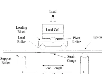
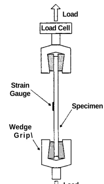
Figure 6.2: Flexural Test Configuration 67

Figure 6.3: Tensile Test Configuration 68

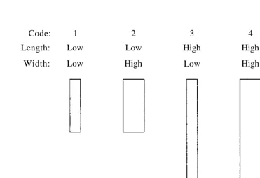
Figure 6.4: Specimen Coding 69

Figure 6.5: Illustration of Main Effects Plot 73

Figure 6.6: Illustration of Interaction Plot 73

Figure 6.7: Hypothetical Data and Fitted Line Illustrating Residuals 74

Figure 6.8: Residual Plots 75

Figure 6.9: Definition of Linear and Quadratic Effects 75

Figure 6.10: Tensile Stress Residual Plots 81

Figure 6.11: Tensile Strain Residual Plots 82

Figure 6.12: Flexural Stress Residual Plots 82

Figure 6.13: Flexural Strain Residual Plots 83

Figure 6.14: Tensile Stress Main Effects Plots 84

Figure 6.15: Tensile Strain Main Effects Plot ....84

Figure 6.16: Flexural Stress Main Effects Plots 85

Figure 6.17: Flexural Strain Main Effects Plot 85

Figure 6.18: Tensile Stress Interactions Plot 86

(9)

Figure 6.20: Flexural Stress Interactions Plots 87

Figure 6.21: Flexural Strain Interactions Plot 87

Figure 6.22: Unidirectional Flexural Failure Stress 93

Figure 6.23: Unidirectional Flexural Failure Strain 93

Figure 6.24: Unidirectional Flexural Failure Stress 94

Figure 6.25: Unidirectional Flexural Failure Strain 94

Figure 7.1: 15-run, Central Composite Design 98

Figure 7.2: W.R. Manufacturer Experimental Series 99

Figure 7.3: Tensile Stress Residual Plots ...110

Figure 7.5: Flexural Strain Residual Plots I l l

Figure 7.8: Flexural Strain Main Effects Plots 113

Figure 7.9: Tensile Stress Interactions Plots 115

Figure 7.11: Flexural Strain Interactions Plots 116

Figure 8.1: Skewed Warp and Weft 122

Figure 8.2: 'Butting System' 123

Figure 8.3: Final W.R. Test Series Structure 124

Figure 8.4: Tensile Stress Residual Plots 132

Figure 8.5: Tensile Strain Residual Plots 132

Figure 8.7: Flexural Strain Residual Plots 133

Figure 8.9: Tensile Strain Main Effects Plots 136

Figure 8.11: Flexural Strain Main Effects Plots 137

Figure 8.12: Tensile Stress Interactions Plots 138

Figure 8.13: Tensile Strain Interactions Plots 138

Figure 8.15: Flexural Strain Interactions Plots 139

Figure 8.16: Tensile Geometry Test Coupons 145

Figure 8.17: Variation of Initial Modulus with Specimen Type 146

(10)

Figure 8.19: Variation of Failure Strain with Specimen Type 147

Figure 9.1 Comparison of Experimental and Published Data 151

Figure C.I: Main Effects Plot C-2

Figure C.2: AxB Interaction C-3

Figure C.3: BxA Interaction C-4

Figure D.I :F density function D-4

Figure F.I: Four-Point Bending F-l

Figure J. 1: Tensile Geometry Tests Homogeneity of Modulus Variance J-l 5

Figure J.2: Tensile Geometry Tests Homogeneity of Failure Stress Variance J-15

Figure J.3: Tensile Geometry Tests Homogeneity of Failure Strain Variance J-16

Figure L.I: Unidirectional Specimen Failures L-l

Figure L.2: W.R. Manufacturer Specimen Failures L-2

Figure L.3: Final W.R. Tensile Specimen Failures L-3

Figure L.4: Final W.R. Flexural Specimen Failures L-4

Figure L.5: Final W.R. Tensile Geometry and ILSS Specimen Failures L-5

Figure L.6: Sample Flexural Load Strain Plot L-6

(11)

List of Tables

Table 2-1: Pertinent Variables 9

Table 5.1: LK(2) Experimental design 55

Table 5.2: "One-at-a-time' Experiment 55

Table 5.3 : L4(2%) Fractional Factorial Design 59

Table 6.1: Experimental design of unidirectional tensile tests 63

Table 6.2: Experimental design of unidirectional flexural tests 63

Table 6.3: Unidirectional Flexural Test Factor Levels 65

Table 6.4: Unidirectional Tensile Test Factor Levels 66

Table 6.5: Instron Cross-Head Speeds 69

Table 6.6: Classification of Factors and Interactions 71

Table 6.8: Modified Whole-Plot and Sub-Plot Sums of Squares Comparisons 79

Table 6.9: Sub-Plot Coefficients of Variation 79

Table 6.10: R-Square Values 80

Table 6.11: Whole-Plot Sums of Squares Normalised with respect to Sub-Plot Error. 83

Table 6.12: Sub-Plot P-Values for Unidirectional Tests 89

Table 6.13: Unidirectional Flexural Strengths w.r.t. Thickness 92

Table 6.14: Unidirectional Flexural Strengths w.r.t. Length 92

Table 6.15: Unidirectional Flexural Weibull Moduli Estimates 95

Table 7.1: 15-Run, Central Composite Design 99

Table 7.2: Flexural Test Geometric Factor Levels 100

Table 7.3: Tensile Test Geometric Factor Levels 101

Table 7.4: Cross-Head Speeds 102

Table 7.6: Whole-Plot and Sub-Plot Sums of Squares Comparisons 108

Table 7.7: Sub-Plot Coefficients of Variation 108

Table 7.8: R-Square Values 109

Table 7.9: Whole-plot Sums of Squares Normalised with respect to Sub-Plot Error.. I l l

Table 7.10: Sub-Plot P-Values for W.R. Manufacturer Tests 114

Table 8.1: Panel Codes 123

Table 8.2: Flexural Test Factor Levels 125

Table 8.3: Tensile Test Factor Levels 125

(12)

Table 8.5: Classification of Tensile Factors and Interactions 127

Table 8.6: Classification of Flexural Factors and Interactions 128

Table 8.7: Whole-Plot and Sub-Plot Coefficient of Variation Comparisons 130

Table 8.8: R-Square values 131

Table 8.9: Summary of P-Values for Final W.R. Tests 135

Table 8.10: Tensile Test Geometry Results 147

Table 8.11: P-values for Identical Means 147

Table 9.1: Comparison of Experimental and Published Data 149

Table 9.2: Comparison of Experimental and Published Data 150

Table 9.3: W.R. E-Glass / Polyester Strengths (11) 152

Table 9.4: Average Strengths 152

Table B.I: Uni-Directional Tensile Tests Results B-2

Table B.2: Uni-Directional Flexural Tests Results B-4

Table C.I: Hypothetical results of an Experimental design C-l

Table C.2: Response Table C-2

Table C.3: Contrast Values C-5

Table D. 1: One factor, two level experiment with five replications D-l

Table D.2: Example Experiment D-5

Table D.3: ANOVA Example D-6

Table E.I: Tensile Correlation Matrix E-l

Table E.2: Flexural Correlation Matrix E-l

Table E.3: Tensile Stress Means and Standard Errors E-2

Table E.4: Tensile Stress ANOVA E-3

Table E.5: Tensile Strain Means and Standard Errors E-4

Table E.6: Tensile Strain ANOVA E-5

Table E.7: Flexural Stress Means and Standard Errors E-7

Table E.8: Flexural Stress ANOVA E-8

Table E.9: Flexural Strain Means and Standard Errors E-10

Table E. 10: Flexural Strain ANOVA E-l 1

Table G.I: Woven Roving Manufacturer Tensile Tests Results G-l

Table G.2: Woven Roving Manufacturer Flexural Tests Results ..G-2

Table H. 1: Tensile Correlation Matrix H-l

Table H.2: Flexural Correlation Matrix H-l

(13)

Table H.4: Tensile Stress Means H-2

Table H.5: Tensile Stress ANOVA H-3

Table H.6: Tensile Strain Parameter Estimates and Standard Errors H-4

Table H.7: Tensile Strain Means H-4

Table H.8: Tensile Strain ANOVA H-5

Table H.9: Flexural Stress Parameter Estimates and Standard Errors H-6

Table H.10: Flexural Stress Means H-7

Table H.11: Flexural Stress ANOVA H-8

Table H.I2: Flexural Strain Parameter Estimates and Standard Errors H-9

Table H.13: Flexural Strain Means H-10

Table H.14: Flexural Strain ANOVA H-ll

Table I.I: Final Woven Roving Tensile Tests Results 1-4

Table 1.2: Final Woven Roving Flexural Tests Results 1-7

Table 1.3: Tensile Geometry Tests Results 1-7

Table 1.4: Interlaminar Shear Strength Tests Results 1-8

Table J.I: Tensile Correlation Matrix J-l

Table J.2: Flexural Correlation Matrix J-l

Table J.3: Tensile Stress Whole-Plot Means and Standard Errors J-2

Table J.4: Tensile Stress Sub-Plot Means and Standard Errors J-3

Table J.5: Tensile Stress ANOVA J-4

Table J.6: Tensile Strain Whole-Plot Means and Standard Errors J-5

Table J.7: Tensile Strain Sub-Plot Means and Standard Errors 3-6

Table J.8: Tensile Strain ANOVA J-7

Table J.9: Flexural Stress Whole-Plot Means and Standard Errors J-8

Table J.10: Flexural Stress Sub-Plot Means and Standard Errors J-9

Table J.I 1: Flexural Stress ANOVA J-10

Table J.I2: Flexural Strain Whole-Plot Means and Standard Errors J-ll

Table J.13: Flexural Strain Sub-Plot Means and Standard Errors J-12

Table J.14: Flexural Strain ANOVA J-13

Table J.I5: Tensile Geometry Tests Descriptive Statistics J-14

Table J.I6: Tensile Geometry Tests P-values for Identical Means J-l6

Table K.I: Unidirectional Reinforcement Details K-l

Table K.2: W.R. Manufacturer Tests Woven Roving Details K-3

Table K.3: W.R. Manufacturer Tests Resin Properties K-4

(14)

Acknowledgements

The Author would like to express his great appreciation of;

Dr. Ajit Shenoi (Department of Ship Science) and Dr. Sue Lewis (Department of

Mathematics) for their encouragement, and expert advice in the fields of composite materials

and experimental design, respectively.

Professor Price for the use of the Department of Ship Science facilities.

Mr. Alan Dodkin and Mr. John Holness at Vosper Thomycroft U.K Ltd. for their valuable

input and the supply of the woven roving laminates and associated data.

Miss Christine Sexton (Department of Mathematics) for her advice and help concerning the

statistical methods used.

Mr. Deryk Taylor (Department of Civil Engineering) for his help and expertise in the testing

of the specimens.

Mr Jim Baker (Institute of Sound and Vibration Research) for the production of the

unidirectional specimens

Dr. Peter Smith and Dr. John MacDonald (Department of Social Statistics) for their advice

concerning graphical modelling techniques

Mr. Ken Yeates (Department of Civil Engineering) for the use of the Instron test rig.

Mr. Mark Foster (Department of Civil Engineering) for his help in cutting out the woven

roving coupons.

Mrs. Jenni Gunn (Department of Civil Engineering/Environmental) for the burn-off tests of the

woven roving coupons.

Miss Jaki Grigg for her help with the burn-off tests and interpretation of the failure mode

(15)

Nomenclature

Chapter 2 b d E F 1 L m M P P T X a

P

e Y X

n

a Chapters a b C C.V. d E F(CT) F,,(a) i K » Breadth Depth Young's Modulus

Force primary quantity

Support span

Length primary quantity

Indicates model

Mass primary quantity

Indicates prototype

Load

Time primary quantity

Secondary physical quantity

Power ensuring dimensional homogeneity

Strain

Power ensuring dimensional homogeneity

Scaling factor

Pi Term

Stress

3 and 4

Half crack length

Breadth

Ratio of maximum to nominal stresses in over-stressed fibre

Coefficient of variation

Depth

Young's Modulus

Probability of failure

Probability of failure of a chain of n elements

ith value in an ordered set of strength values

Stress intensity factor

(16)

Ks 1 L m mb md m, n N N P Q,(CT) r * S(o) U.D.L V X y z 5 s q>(c)

n

e

a Of CTMax a.

Stress distribution factor Length

Length of fibres

Weibull shape parameter or modulus

Weibull modulus in breadth direction

Weibull modulus in depth direction

Weibull modulus in length direction

Number of elements

Number of fibres around each i-plet

Number of fibres

Number of values in an ordered set of strength values

Load

Number of i-plets present

Number of i-plets created

Distance between crack tip and elemental volume

x-axis extent of plastic zone

Probability of survival

Uniformly distributed load

Volume Cartesian co-ordinate Cartesian co-ordinate Cartesian co-ordinate Ineffective length Strain

(Weibull) Distribution function

Effective length

Pi Term

Angle between crack and line joining crack tip and elemental volume

Stress

Stress corresponding to critical stress intensity factor

Stress at which first i-plet appears

Stress at which i-plets become unstable

Maximum stress in over-stressed fibre

(17)

ault ays X Chapter 5 a ab abc ac b be c y a

P

8 8 Y Tl Chapters 6, B CW CL 1 md m, mv M Mod q R

Wei bull threshold stress Ultimate strength

Yield stress

Weibull scale parameter

Shear stress

Coded value of factor A

Coded interaction between A and B

Coded interaction between A, B and C

Coded interaction between A and C

Coded value of factor B

Coded interaction between B and C

Coded value of factor C

Response variable Unknown parameter Unknown parameter Unknown parameter Random error Unknown parameter Unknown parameter Unknown parameter 7and 8 Butts factor

Coded width factor

Coded length factor

Indicates linear effect

Weibull modulus based on depth

Weibull modulus based on length

Weibull modulus based on volume

Woven roving manufacturer factor

Initial Modulus

Indicates quadratic effect

(18)

s

T Vf X Y a Skew factor Thickness factor

Fibre volume fraction

Hypothetical factor

Hypothetical response variable

Hypothetical Y-axis intercept

Coefficient corresponding to effect of ith factor

Intercept

p

£ E E ^lens.ult ^tens.ult °flex.ult ^flex.ult Appendix A i k M N Pi Qk Qn r x,

n

Hypothetical effect of X Sub-plot error

Hypothetical Random error

Whole-plot error

Ultimate tensile stress

Ultimate tensile strain

Ultimate flexural stress

Ultimate flexural strain

Exponents in physical equation

Number of Pi terms

Number of primary physical quantities

Coefficient in physical equation

Dimensionless number

ith secondary physical quantity

kth primary physical quantity

nth physical quantity

Ratio of similar physical quantities

Exponents of ith Pi term

ith Pi term

Appendix D

fa Pooled degrees of freedom

F F-ratio

Ho Null hypothesis

(19)

nR Number of experimental replications

N Total number of responses

Sj2 Variance of high and low averages about the mean

sR2 Variance for Rth factor level

S2 Pooled variance

SSO pooled sum of squares

y Average response for experiment

yR Average response for R t h factor level

yR i Response variable for ith replication of Rth factor level

a Significance level

fi Average response

u, F-ratio degree of freedom

(20)

1. Introduction

1.1 Composite Materials

A composite structural material consists of more than one phase at a macroscopic scale. The

mechanical properties of the composite are designed to be superior to that of the constituent

materials considered independently. Usually, two phases are present, a stiff, strong

reinforcement set in a less stiff and weaker matrix. The characterisation of these materials

ranges from low performance composite materials, where the reinforcement usually consists

of short fibres or particles and the matrix is the main load bearing constituent, to high

performance composites, where continuous fibres carry most of the load in the direction of

their alignment. The matrix of a high performance composite supports and protects the fragile

and unstable fibres, and also serves to transfer load to and between the fibres. The interface

between the two phases can be very important in controlling the failure of the composite. The

materials considered in this study are fibre reinforced plastic composites, or F.R.P. , where

the fibres are set in a synthetic polymer.

The first fibreglass boat was made in 1942 by the US Navy, this was followed by larger craft,

and 1979 saw the completion of the first 60m, all F.R.P. vessel, HMS Brecon. These

materials are now common throughout the marine industry, and are used in the construction

of windsurfers, dinghies, canoes, speedboats, yachts, workboats, lifeboats, submarines,

offshore platforms and Navy patrol boats and minehunters. The vast majority of marine

composites use E-glass fibres, most commonly in the form of a balanced woven roving, in a

cold-curing polyester resin matrix. Usually such composites are fabricated using contact

moulding in an open female mould using 'spray-up' or 'hand lay-up' methods. Spray-up

entails the incorporation of short glass fibre rovings into a stream of resin which is sprayed

onto the mould. Hand lay-up involves the successive laying down of reinforcement material

plies onto a liberally applied layer of resin, followed by wetting out and consolidation by

rolling or brushing into this wet resin. Some automation of the lay-up process has been

achieved, but unless constant production is required, inactive periods require uneconomical

cleaning of the equipment between production runs. These techniques lead to composites

with generally lower and more variable mechanical properties than those commonly used in

the aerospace industry, where the fibres are pre-impregnated with resin in a controlled

(21)

1.2 Seating Problem

The relatively recent introduction of FRP composite technology, together with the large range

of materials used and being introduced, mean that a broad design base, such as that available for

many metals, has not yet been compiled for FRP materials. Hence much testing of composite

components has to be carried out either on full scale prototypes, or, in order to save both time

and expense, on small scale models using the principles of dimensional analysis. It follows

therefore, that any discrepancies encountered whilst scaling from model to full size (i.e. any size

effects) should be both identified and understood. Similarly, much of the design of composite

components is based on material properties derived from small laboratory scale coupons, often

leading to a trial and error approach if the properties obtained in the laboratory tests do not

correctly predict the component behaviour.

It has been thought for some time that a strength 'size effect' may exist for some composites,

which is usually (but not exclusively) detrimental with increasing size. This is thought to be due

to the increased probability of a larger specimen containing a flaw large enough to lead to

failure. However, an accurate quantitative description of such effects, or even concrete evidence

of their existence, has proved elusive. These problems may be compounded by the fact that a

separately manufactured specimen will not necessarily have the same properties as a

comparable specimen cut from the full scale structure. This latter effect is due more to the scale

of production than to the actual size of the composite laminate considered. Hence it may be

helpful to think of this as a 'scale effect' rather than a 'size effect'.

The scaling problem is especially complex for composites due to the intricate nature of their

micro-structure. Difficulties arise when it becomes either very difficult, or impossible to scale,

for example, such elements as fibre diameter and fibre / matrix interface. The 'custom-made'

nature of composites introduces further complications, as there are many possible material

variables to be considered, such as manufacturing route, manufacturing conditions, fibre and

matrix materials, stacking sequence, fibre volume fraction and void content.

Similarly, the measured mechanical properties of composites are dependent on testing variables,

such as test method, environmental conditions, test set-up, specimen geometry, failure mode

(22)

problem of testing standards comprises a whole field of research on its own and is considered to

be outside the scope of this study.

Other features of composites testing are the high degree of experimental scatter obtained in the

mechanical properties obtained, and also the difficulty encountered in repeating such results.

This is especially relevant for hand laid up marine composites, whose mechanical properties are

much more variable than those of aerospace pre-preg laminates.

1.3 Aims

The aim of this study has been to investigate the existence of 'size effects' which affect the

strength of composites used in the marine industry. A test programme at the coupon scale has

been completed in order both to identify the relevant important factors and also the manner in

which they interact. Statistical experimental design methods have been used to plan and

analyse the results of this test programme, and the sources of the variability commonly seen

in composites empirical strength data are investigated. The materials covered in the study

include E-glass and carbon reinforcements set in epoxy and polyester matrices. The

reinforcements include uni-directional (UD) and woven roving (WR) cloths. The effects of

(23)

2. Engineering Experimental Modelling

2.1 Background

There are many texts concerning experimental modelling and the field of dimensional

analysis. David and Nolle (1982) provide a very thorough yet clear explanation from an

engineering point of view, and a similar approach is also taken by Murphy (1950) and Emori

and Schuring (1977). Langhaar (1951) provides an account of the theory of models with

respect to dimensional analysis. Texts mainly concerning dimensional analysis include

Isaacson and Isaacson (1975), Barenblatt (1987), Taylor (1974), and Bridgman (1922).

The use of scale models by engineers in order to predict the performance of the full scale

article has been an integral part of the design process for centuries. The first "modern"

scientist to do so was Cauchy, who investigated the vibration behaviour of model plates and

rods in 1829. In 1869 W. Froude made the first models for use in a water-basin in order to

predict full scale ship performance, and in 1883 O. Reynolds carried out his classic model

experiments on the motion of fluids in pipes. The beginning of the century saw the Wright

brothers successfully complete the first heavier than air powered flight in an aircraft designed

using scale wing models in a wind tunnel.

There are many fields of application of scale models including architecture, aerospace

engineering, hydrology, meteorology and geophysics, but the oldest and best known is that of

naval architecture. An important part of the design of any ship involves model testing;

frictional and wave-making resistance, propeller performance, manoeuvrability, ship bending

and vibration and sea-keeping are all investigated using this technique. The design of large

and complex structures also uses model prediction extensively, although this is being

replaced by computational methods such as finite element analysis. However, the use of such

computational methods with composite materials is limited by factors such as the lack of

material data available and the complexity and inherent variability of the material system.

Hence model construction, testing, re-designing and re-testing, often many times, is still an

integral part of composite component design.

The use of experimental modelling may well reveal factors or behaviour that would not have

(24)

current strong tendency toward computerisation, the researcher in physical and engineering

sciences relies more than ever on experimentation. More theory demands more testing, not

less; otherwise, the theorist would drift toward playing mere games." Further, the limitations

of experimental data must also be remembered; the data obtained through model tests is

empirical in nature and does not necessarily disclose any underlying physical laws. Hence

care must be taken when extrapolating outside the ranges of the variables considered.

There are, broadly speaking, three methods of predicting the performance of an engineering

structure (Murphy (1950));

(i) The physical laws concerning the system are used to give a mathematical model

and the system performance is predicted using this analysis,

(ii) The structure itself is fabricated and tested before use,

(iii) Tests are conducted on a scale model.

The first method becomes impractical for complex structures concerning many variables and

the designer must be confident that the theories used are not only correct but also complete.

The second method has the obvious drawback of being both expensive and time consuming

unless small, easily fabricated items are in question. This often leaves model experiments as

the most reliable yet cost effective route to final product design.

The purpose of an experimental engineering model is often to gain information about the

behaviour of the full sale component or prototype through tests conducted on an easier to

manage model. By "easier to manage" we may mean that the model is smaller, for example

when considering a ship, or that the process takes a much shorter time at model scale, for

example river sedimentation problems. It must be noted that these cases are only examples;

the model may be larger than the prototype if the latter is too small to be easily manipulated.

However, in the field of composite structure design the models are usually smaller than the

prototype for reasons of economy. Experimental modelling may also be used for purposes

other than the design of an engineering product, such as the investigation of physical

processes. This is particularly true for those phenomena where the effect of scale is thought to

(25)

In order for the use of experimental model scale testing to be successful it is imperative that

the unique relationship between the behaviour of the model and that of the prototype is well

understood. It must be known that the model and prototype obey the same physical laws and

that all the relevant features are correspondent if the model data is to be extrapolated to full

scale. The unique relationship between model and prototype is broadly referred to as

similarity and the conditions required to ensure similarity are developed using a technique

known as dimensional analysis which is based on our concepts and conventions of

measurements and observations.

2.2 Dimensional Analysis

The use of dimensional analysis is directed towards finding pertinent non-dimensional

combinations of variables for the physical system. These terms are subsequently employed in

order to ascertain the required relationships between model and prototype. There is no one set

of algorithms that the experimenter may follow in order to come to the correct relationship;

there is no one correct method. Much is left up to the experimenters knowledge of the field

and ingenuity. In fact Emori and Schilling (1977) describe scale modelling as an art rather

than a technique and points out that each problem must be treated anew.

In the field of mechanics it is usual to describe systems using three "basic", or primary

quantities, mass (M), length (L) and time (T). Mass is often replaced with force (F) by

engineers (through the use of Newton's second law), since this more directly corresponds

both to the measurements taken and to the results required. The choice of primary quantities

is purely arbitrary in much the same way as is the measuring system we have chosen to adopt.

The primary quantities must, however, satisfy three conditions;

(i) They must be mutually independent,

(ii) They must be measurable,

(iii) They must be sufficient in number to define the dimensions of every pertinent

variable.

The methods of dimensional analysis are based upon two principles inherent to the

(26)

(i) The ratio of the magnitudes of two like quantities is independent of the units used,

if the same units are used for both quantities,

(ii) General relationships may be established between two quantities only when they

have the same dimensions.

From these axioms follows the concept of an homogenous equation which is defined as an

expression which remains valid for any measuring system used throughout the equation in

question (David and Nolle (1982)).

Any variables pertinent to the system considered may be expressed as functions of the

primary quantities, examples of such secondary quantities include stress and velocity. Using

the concept of homogenous equations it can be shown (David and Nolle (1982)) that the

dimensions of any such physical quantity (x) can be expressed as the product of powers of the

primary quantities of the system;

(2-1)

where a, p and y are powers ensuring dimensional homogeneity.

The basis of the mechanics of dimensional analysis is the use of non-dimensional groups or

Pi terms after the "Pi-theorem" as set out by Buckingham (1914). The use of such groups not

only enables similarity conditions between model and prototype to be established but also

reduces the number of variables that has to be considered. This may save the experimental

effort required considerably. There are three main methods of obtaining non-dimensional

groups;

(i) The system equation approach,

(ii) Rayleiglvs method,

(iii) The Buckingham-Pi method.

The first method is dependent upon a thorough knowledge of the system concerned and a

complete mathematical analysis to yield the system equations. These equations are then

normalised to give non-dimensional groups. The method has the advantages that, once the

mathematical model has been established and solved, the extraction of the non-dimensional

(27)

However, the mathematical model may be unknown, too complex, too time consuming or

even insoluble, requiring alternative methods for obtaining Pi terms. The Rayleigh and

Buckingham-Pi methods use dimensional analysis to identify Pi terms. The reader is directed

to David and Nolle (1982) for an explanation of the former and to Appendix A for the

background and theory of the latter.

The results of both dimensional analysis approaches are more easily interpreted and utilised if

the non-dimensional groups relevant to the problem are selected, i.e. terms which have some

physical meaning are advantageous. To do this requires an understanding of both the physical

processes and the relevant variables of the system. It is hence also important that initially all

the pertinent variables are selected. Omission of any variables involved in the system

processes will result in errors in the prediction of prototype behaviour from model

experiments. Conversely, selection of unnecessary or uninvolved variables may not affect the

validity of the model, but may entail unnecessary complexity, possibly obscuring the physical

relevance of the non-dimensional groups developed.

As previously mentioned, there is no one set of algorithms which provides a single path to the

dimensional analysis, and so it is easiest to provide a simple example to illustrate how the

technique is applied. Consider the example of the four-point bending of a thin beam as shown

in Figure 2.1;

b

O

(J

1/3

1

IT

O

o

Figure 2.1: Four-point bending

Firstly the pertinent variables are selected. For this example it is initially assumed that the

only relationship known to apply to the variables of the system is that shown on the right

hand side of Figure 2.1. i.e. that the specimen material behaves in a linearly elastic manner;

G = Ee ( 2.2 )

(28)

The pertinent variables and their respective dimensions are given in Table 2-1.

Variable 1

P o 8

E b d

Definition

Support length Load

Stress Strain

Young's Modulus Specimen width Specimen depth

Primary Quantity L

F FL-2

[I] FL-2

L L

Table 2-1: Pertinent Variables

The number of independent Pi terms required is equal to the difference between the number of system variables and the number of primary quantities involved. In this case there will be 5 Pi terms.

Once the relevant variables have been identified the Buckingham Pi theory is applied. Taking 1

and P to be the fundamental units;

ni=IaiP'ntr (2.3)

This equation must be dimensionally homogenous, i.e.;

(2.4)

Hence; LalFfilFL~2 = L°F° (2.5 )

Equating indices gives; ax=2 ( 2 . 6 )

i.e. / V (2.7)

1 P

Similar procedures give;

U2=£ (2.8)

„ 12E (2.9)

_ * (210)

(29)

It is perhaps not surprising that strain appears as a Pi term, since it is already defined as a

non-dimensional quantity.

2.3 The Theory of Models

Once a set of Pi terms has been identified the next step is to use them to give the relationship

between model and prototype behavior. It is convenient to consider two types of Pi terms, the

test parameter and the design parameters or conditions. The test parameter is the Pi-term

containing the variable which is to be predicted and the design conditions are those containing

the other system variables. As is normal engineering practice the system or prototype is

expressed as a relationship between the parameter to be predicted and those which can be

measured;

n

1

=F(n

2

,n,,n

4

,...n

5

.) (2.12)

where ITi is the test parameter and II2 to Ils are the design conditions.

For the four point bending example considered above, the stress in the beam could be of

interest. If this is the case then the Pi term containing this variable (TIi) would be taken as the

test parameter;

I2a J b d\ (2.13)

Since equation ( 2.12 ) is entirely general it also applies to the model system since the latter is

a function of the same variables;

n

lm

= F{n

2m

,n

3a

,n

4m

,...n

Sm

,) (2.14)

where the subscript m denotes model.

Therefore the relationship between prototype and model may be expressed as;

n,

=

F(n

2

,n

3

,n

4

,.,.n,,) (2.15)

(30)

Take the case where that all the test parameters are equivalent between prototype and model;

i.e. n2= n2 / H (2.16)

n, =

n,,,,

etc.

Since the function F is the same for model and prototype, it follows that;

n , = n

l m

(2.17)

The prediction equation ( 2.17 ) is valid if all the design conditions are satisfied, i.e. if

equations ( 2.16 ) are true. In this case there is complete similarity and all of the relevant

aspects of the prototype are faithfully reproduced in the model.

Complete similarity can be further subdivided into distinct types of similarity relating to

specific Pi terms. For example if a Pi-term contains only geometric variables, such as length,

width, depth or angles, and the design condition concerning this Pi-term is satisfied then

geometrical similarity is said to exist. This is the most obvious interpretation of the term

similarity, but many types may be defined including those concerning;

(i) Geometry,

(ii) Material properties,

(iii) Forces, moments etc.,

(iv) Mass distribution,

(v) Timing,

In the case of complete similarity there is said to be a true model and predictions using this

model will be accurate, if all the pertinent variables were included initially.

The design conditions must now be met through manipulation of the system variables. In

order to do this the ratio of a variable for the prototype to its value for the model is defined as

a scaling factor. For example, for variable X;;

, *-, (2-1 8>

(31)

From this definition it follows that for similarity the corresponding scaling factor for a Pi-term should have a value of one;

i e . n , , (2.19)

A 1

Expressing each design condition or Pi-term as a function of the relevant variables, x,;

i-e- n , = / ( x , ) (2.20)

Hence, for complete similarity;

The equations (2.21 ) can then be used to give the required scaling factors. The number of design scaling factors which may be independently varied is limited to the difference between the number of variables and the number of Pi terms. For the previous example of four point bending of a beam, this would amount to only two variables. Returning to this example will illustrate how the model variable values may be derived from the equivalent prototype values and the Pi terms resultant from the dimensional analysis. Firstly, restating the test parameter and including its scale factor form;

n l2o . . _%K (2-22)

n

'"T" '

ni

~~I7

The corresponding equations for the design conditions are;

n2 = e ; Am = A£ (2.23)

n

-tE.

x

-£h.

(224)

3" P ' m~ AP

n =* •

A

= ^

( 2 2 5 )

4 / ' n4 A,

n =f f . ^ = Ad_ (2.26)

5 / ' n5 A;

(32)

Xa=l ; A, =10 (2.27)

This means that the two variables which may be independently varied have been set and the equations ( 2.22) to ( 2.26) provide the values of the other five;

; A, = l (2.28)

Xb = 10 ; kd = 10

Hence, if the model is scaled geometrically by a factor of 1/10 then in order to achieve the same stress strain state as in the prototype a load of 1/100 that at full scale must be applied.

To summarise the procedure for the use of a completely similar model;

(i) List all the relevant system variables,

(ii) Employ dimensional analysis techniques to give a set of non-dimensional Pi terms, (iii) Set the values of the required scaling factors

(iv) Use the requirement that all Xm must be unity to give the other scaling factors, (v) Use the scaling factors together with the prototype variable values to give the corresponding model values.

Murphy (1950) devotes a whole chapter to the application of completely similar experimental models to structural problems.

2.4 Distorted models and Scale Effects

(33)

distortion is usually simply that the loads applied to the model are either too large or too

small to ensure similarity, but these forces can also be applied at non-commensurate

positions. Material properties distortion may occur because, for example, the Young's

modulus or Poisson"s ratio of the material used to fabricate the model is not the same as that

of the prototype. It may also be because of different stress strain behaviour of the model and

prototype, especially if non-linear elastic or plastic behaviour occurs.

A distorted model may arise either because it is not possible to set all the variables in order to

achieve complete similarity, or because it is not desired to. Using the previous example to

illustrate this, it may not be practical to produce a beam of one tenth of the width of the

prototype to the required precision. It could also be that the way in which the width of the

beam affects the strength independently of the length is of interest. In either case some

recourse must be taken to reconstitute the relationship between model and prototype. Usually

additional knowledge in the form of an equation not used in the dimensional analysis

performs this task.

Returning once more to the beam bending example, if the width of the model is twice the

value for complete similarity, then what is the required load to achieve equivalent stress

states? This may be found from the equation developed from simple beam theory linking the

maximum stress in the beam to its geometry and the load applied;

PI ( 2.28)

cr = bd2

From this it can be seen that the applied load must be twice that for the completely similar

model, i.e. the value of XP must be 50. Murphy (1950) devotes a whole chapter to the subject

of distorted structural models.

It is convenient here to illustrate how using the system equations produces the relationship

between model and prototype variables by a more direct route than does dimensional

analysis. Expressing equation ( 2.28 ) in terms of scaling factors gives;

(34)

It is then relatively easy to produce a set of the scaling factors on the right hand side of

equation ( 2.29 ) to give a value of Xa of unity.

Once the analysis has been completed the prototype behaviour may be predicted from the

experiments performed on the model. It is often the case that on construction of the prototype

these predictions are found to be inaccurate to some degree. This is often referred as a "scale

effect", since the scale of the system appears to affect its behaviour. However this is simply a

name given to an unknown phenomenon which has not been included in the initial appraisal

of the system and hen?e the scaling relationship used. In other words the model is still

distorted since we have not allowed for all the features of the system considered. David and

Nolle (1982) suggest some reasons for such differences between model and prototype

behaviour;

(i) Some effect may be insignificant at prototype size but significant at model size or

vice versa. For example the effect of surface tension on storm waves is slight whereas

this force will have a large effect upon the waves produced in a laboratory scale

hydrological model of an estuary.

(ii) There may be a change in behaviour. For example the flow regime may change

from laminar to turbulent.

(iii) Measurement or construction accuracy may be different for different scales. For

example it may be easy to fabricate a one metre prototype to a tolerance of one

millimetre, but impossible to obtain the equivalent tolerance for a one centimetre

model.

(iv) The material properties are affected by scale. This may be due to differences in

fabrication methods, for example.

Some of these points will be addressed with respect to marine composite structures in

Chapters.

From a design point of view such scale effects may be allowed for using previous model and

prototype scale experimentation experience to give "engineering" factors. A more scientific

approach is to carry out experiments on a range of scaled systems with the view to use the

(35)

in Chapter 4. it is thought that such a scale effect may occur for certain composite materials.

In order to try to quantify and explain any such effects the second approach is taken here

(36)

3. Analysis of Size Effects

In order to enable accurate design, any scale effects concerning the material properties of

fibre reinforced plastic composites (see Section 1.2 and Chapter 2) need to be identified,

understood and then compensated for. Here, the methods used to describe such effects, both

quantitatively and qualitatively, are outlined. In section 2.4 four possible causes for scale

effects were suggested. When considering the strength and stiffness of a structural material

such as fibre reinforced composites it is possible to rationalise these into two main categories;

(i) Differences due solely to the amount of material considered,

(ii) Differences between model and prototype due to construction techniques and

conditions, difficulties in scaling certain variables and other distortions.

The first category has been the main preoccupation of the literature on the subject of material

strength scaling (see Chapter 4). The underlying principle here is that the strength of brittle

materials is controlled by the presence of defects, or flaws in the material and that a larger

amount of material will contain more of these flaws. This approach is often referred to as

statistical strength theory and is considered in sections 3.1 and 3.2.

The second category is far more wide ranging, but generally concerns the different

implications of constructing structures at small scale and at large scale. For example, the

small scale process may take place under carefully controlled laboratory conditions whereas

the large scale process may take place in a workshop environment. It may also be difficult to

scale exactly between prototype and model due to physical constraints on the system. Section

3.3 considers these types of effect. A possible distortion of the similarity across scale is

suggested by linear elastic fracture mechanics (L.E.F.M) and the background to this theory is

given in section 3.4.

3.1 Weakest Link Theory

Statistical strength theory or statistical weakest link theory has formed the basis of

conventional brittle fracture study for many years. The concept of the weakest link was first

used by Pierce (1926) to investigate the strengths of long lengths of cotton yarns by

considering them to made up of shorter lengths linked together. Shortly after this study,

(37)

the subject, giving his name to the most widely used distribution used in weakest link theory

and showing that the theory could be applied to many brittle materials. More research in the

field by Epstein (Epstein (1948a), Epstein (1948b)) recognised the close relationship between

weakest link theory and the statistical theory of extreme values.

Weakest link theory is based on the assumption that the material is made up of smaller

elements linked together and that, like the links in a chain, failure of the material as a whole

occurs when any one of these elements or "links" fail. The probability of failure of each link

subjected to a stress increase from 0 to a is described by the distribution function F(a). The

probability of survival of that link is then given by;

It is also assumed that F(c) describes the strength distribution for every element and that each

F(a) is an independent randomly distributed variable. The probability of survival of n

elements in series is then given by;

» [ ( ) ] "

(3.2)

Hence the probability of failure of a chain of n elements is given by;

= \-[\-F(*)]' (3.3)

Equation ( 3.3 ) forms the basis of statistical weakest link theory. The equation shows that,

since F(a) must be positive and less than one, for a given stress level a, as the number of

elements increases so does the probability of failure. In other words as the chain becomes

larger it becomes weaker and a scale effect has been described.

The function F(a) may be described generally as;

F(o-) = l-exp[-^(c7)] ( 3 > 4)

The function cp(o) must be positive, non-decreasing and tend to zero at a specified value of a,

au say, in order to give a form of F(a) comparable with material strength behaviour. Hence to

(38)

A specific form of cp(cr) was put forward by Weibull (1939) and is still used widely today. He

describes it as the simplest mathematical function which is positive, non-decreasing and tends

to zero at a value of a of au. This function has become known as the "Weibull distribution"

and is given by;

.j^J°-°,,) (3.5)

(3.6)

i.e.

F(o) = 1 - exp a-a,,

Where a,, is the threshold stress below which failure does not occur and a0 and m are called

the scale parameter and the shape parameter respectively. This form is termed the three

parameter distribution.

Weibull does not argue any theoretical reasoning behind the derivation of this function, but

simply states that it fits many real data sets and is also simple to use. This leads to a

probability of failure of n elements in series of;

o-cr,.V'l (3.7)

For the strength of a material subjected to an increasing load from zero to a there is zero

chance of failure only when there is no applied load. This means that au is usually taken to be

zero and hence the two parameter form is used;

( 3 . 8 ) = l - e x p -n

Considering a volume of material comprising of small elemental volumes, 8V, instead of a

chain of "links" gives;

( 3 . 9 )

1 \.t)

dV

For tensile testing the stress o is uniformly distributed through the material volume. Initially

(39)

(3.10)

In order to use this equation to describe experimental data it is convenient to express equation

( 3.10 ) in a linear form. Rearranging and taking logarithms twice gives;

In In 1 = m ln(cr) - m ln(cr0) + ln( V) (3.11)

Hence a plot of ln(a) versus the left hand side of this equation for N replications of an

experimental strength test for a given volume of material, V, will give a linear relationship if

the material strength variability is described by the Weibull distribution. From the slope and

y-axis intercept of this line both the shape and scale parameter respectively may be estimated.

Varying the volume of material translates the line vertically as shown in Figure 3.1 .

V

ln(c)

Figure 3.1: Logarithmic Plot of Weibull Strength Data

The calculation of Fv(o) for a set of experimentally obtained stresses, a, can be carried out

using a statistical approximation technique as described by Weibull (1939). Here the N values

of a obtained for a given volume, V, are arranged in ascending order, and for the i^ value ;

ir,(CT) = _ L _ (3.12)

Alternatively, the shape parameter m may be approximated from the coefficient of variation

(40)

m^C.V.-1.22 _{( 3.13 )}

Similarly, Hitchon and Phillips (1978) quote;

12

m w

C.V. (3.14)

Considering the more general case of a varying stress field through the material volume. In

Cartesian co-ordinates;

a = cx{x,y,z) ( 3 1 5 )

Hence, from equation ( 3.9 );

dV (3.16)

On integration we can express this generally as;

(3.17)

Where Ks is a factor dependent upon the stress distribution and ar is a reference stress at a

specific point in the material.

For tensile tests the stress distribution is uniform and hence K, has a value of one. The

derivation of Ks for four-point bending is given in Appendix F and results in;

m + 2

K = (3.18)

If the strength distribution of a material is described by Weibull theory then it is possible to

correlate the strengths of specimens or components of differing size. An assumption is made

that the values of the shape and scale parameters m and CT0 are material constants,

independent of the size of the specimen and its stress field. Considering two specimens of

(41)

•y, = 1 - exp (3.19)

Fr2 = l - e x p

Assuming that we are interested in the same probability of failure at each size, for example

the mean strength with a probability of failure of 0.5, gives;

a (v\~» (3.20)

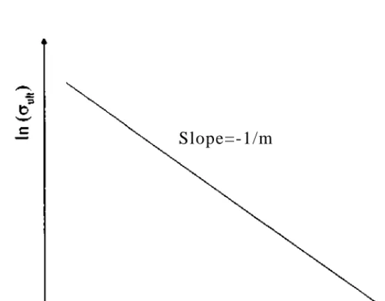
This equation directly links strength to volume and hence quantifies the size effect. A

logarithmic plot of stress versus volume gives a straight line relationship of slope -1/m, as

shown in Figure 3.2 .

Slope=-1/m

[image:41.548.138.415.309.526.2]

ln(V)

Figure 3.2: Logarithmic Plot of a Strength Size Effect

We can extend this approach to include the effect of differing stress distributions by using

equation ( 3.17 ) to give;

This equation again quantifies the size effect but also includes the influence of differing stress

(42)

For anisotropic materials such as fibre composites both the strength distributions and the

effects of flaws in differing directions may not be the same. Integrating equation ( 3.9 ) over

length instead of volume, for example gives;

Similarly for breadth and depth;

n. (hXk (3.23)

a,

S^Jd^ <

3

'

24

>

o

x

[dj

Where mi, nib and ma are not necessarily equal.

The theory as applied to anisotropic materials is referred to as modified weakest link theory.

Although almost all of the literature on composite materials concerns the Weibull distribution

many others are available. Other distributions which have been considered include the

rectangular and Laplace distributions (Epstein (1948a)).

3.2 Extensions of Weakest Link Theory for Composite Materials

Weakest link theory accurately describes the failure of brittle materials. However, although

most composite materials fail at very low tensile strains, final failure generally occurs after

some damage accumulation. There is much available literature suggesting the constituent

fibres of many composites do behave as brittle materials (Moreton (1969), Metcalf and

Schmitz (1964), Watson and Smith (1985), Padgett et al. (1995)). This is one of the

assumptions of the theory first put forward by Rosen (1964) and Zweben and Rosen (1970),

but damage accumulation is also taken into account. The solution of the damage accumulation

problem proffered by Zweben and Rosen involves many simplifications and assumptions.

Further work by Harlow and Phoenix (1978a) and Smith (1980) gave comprehensive exact

mathematical solutions. However these more complicated models also require the estimation

(43)

comparatively large and so the simpler and more easily interpreted theory of Zweben and

Rosen is outlined here, as described in more detail by Batdorf (1990). The bundle of fibres

model, as first suggested by Daniels (1945), is in fact an extension of simple Weibull theory. A

chain of elements is again considered, but in this case the elements are assumed to consist of

many fibres, as illustrated in Figure 3.3.

Figure 3.3: Bundle of Fibres Elements : , . . . , , ,

Daniels assumed that for a loose bundle of fibres when an individual fibre failed, the bundle as

a whole did not fail due to redistribution of the load equally among the other fibres. However,

a fibre reinforced plastic composite material consists of high stiffness and high strength fibres

embedded in a relatively low modulus weak polymer matrix. The fibres in an undamaged

unidirectional uniaxially loaded composite carry the majority of the load. In a similar manner

to Daniels, Zweben and Rosen hypothesised that when the first of these fibres failed the

composite as a whole did not fail, because of load transfer by the matrix. However, they

supposed that the load previously taken by the broken fibre is now transferred via the matrix

only to the adjacent fibres, around the break and then back to the original fibre. A

consequence of this shear transfer is that, for a certain length either side of the break, the

failed fibre carries less load whilst those adjacent carry more. This is shown in Figure 3.4.

Matrix \

• -':: I ' -" V . "

CT | *

..:-:,: , ::; x:x:;:;:

CT

'mm'^w v ""

m

^

1

. / | \

CT j . VS;;S:::s

\ :

\ •

/

/ - • ' : •

i

[image:43.551.51.498.21.254.2]

T E N S I O N

(44)

The length over which this shear transfer occurs is known as the "ineffective length" denoted

by 5. Despite the fact that the adjacent fibres now carry more load, since 8 is small the

probability of a critical flaw occurring in this length is also small and hence failure is

unlikely. Also the excess load is shared amongst all neighbouring fibres and so the load

increase is not large.

This type of isolated fibre breakage is termed a "singlet" and as the load is increased more of

these will appear. As the load is further increased it becomes more likely that the over

stressed parts of the adjacent fibres should themselves fail. When this occurs there are two

adjacent broken fibres and this is termed a "doublet". Still further loading will give rise to

more singlets and doublets and then "triplets". This continues until a critical "multiplet"

occurs and the process becomes unstable, resulting in the failure of the composite as a whole.

Considering the two parameter Weibull distribution;

a) (3.25)

For the fracture of a fibre this may be interpreted as the number of defects unable to sustain a

stress a per unit length of fibre. Hence the number of singlets formed in N fibres of length L

is;

4^1"

(3J6)

This assumes that the ineffective length 5 is much less than the fibre length L. A further

assumption is that N is large so that the number of flaws at the edges of the composite and

hence not surrounded by other fibres is small.

In order to simplify the analysis the ineffective length for a singlet 5, is replaced by a

conceptual '"effective length" A.,. Each fibre adjacent to a singlet has a maximum increase in

stress in the plane of the break. The effective length is that which, when subjected to this

maximum stress, has the same probability of failure as the ineffective length subjected to the

(45)

Figure 3.5: Ineffective Length (8) and Effective Length (k)

The total length of overloaded fibres surrounding the Q, singlets is hence Qin,^, where n, is

the number of fibres around each singlet. Defining the ratio of aMax to a as C, gives the

number of failures expected in this length as;

n nr,A

C

^Y

( 3

'

2 7

>

This is the number of singlets converted to doublets at stress a and may be generalised to

higher order multiplets;

QM = C.a (3.28)

This is not generally equal to the number of i-plets present at load a since some will have

been converted to higher order multiplets, the actual number is hence;

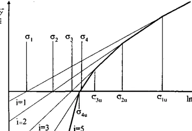
It can be seen from equation ( 3.28 ) that a logarithmic plot of Q< against a for the ith

(46)

'3u J2u ' l u

[image:46.553.120.438.19.236.2]

1=

Figure 3.6: Logarithmic Plot of the Bundle of Fibres Model

Using this graph it is possible to predict the failure behaviour of the material as the stress is

increased. As the stress is increased the first fibre failure occurs at a, where the singlet (i = 1)

line cuts the In Q, = 0 line, i.e. where the number of singlet failures is one. Simple Weibull

theory, whereby the initial failure is said to lead to catastrophic failure would predict failure

of the material as a whole at this point and the i = 1 line does in fact correspond to this

theory. However failure does not occur in this case and further increase of stress results in

more singlets and at a, the first doublets are formed. Since all doublets are formed from

singlets there can never be more doublets than singlets. Hence at CT1U the i = 2 line follows that

for i = 1. Above this stress any singlets formed are unstable and are immediately converted

into doublets. From this it is apparent that failure of the material occurs when the stress at

which a certain multiplet first appears is equal to or greater than that at which it is unstable.

i e- a'*°* (3.30)

This occurs when the envelope of the Q{ lines indicated in bold in Figure 3.6 cuts the ln(cr)

axis. For the case in Figure 3.6 further increase in stress from a2 results in more singlets and

doublets until, at a:, the first triplets are formed. Further stress produces more singlets,

doublets and triplets. At a4 the first quadruplet is formed, but this is unstable and failure of

the material results.

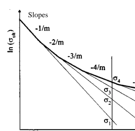
From equations ( 3.26 ) to ( 3.28 ) it is apparent that the number of multiplets is proportional

(47)

V. Hence a change in V translates the lines in Figure 3.6 vertically, changing the values of the

intercepts with the ln(a) axis. This relationship may be represented on a logarithmic plot of

failure stress against NL, as shown in Figure 3.7. This plot is analogous to that for simple

Weibull theory (see Figure 3.2).

Slopes

-5/m

[image:47.551.162.395.113.339.2]

ln(NL)

Figure 3.7: Logarithmic Plot of Bundle of Fibres Model

The failure line is again the bold line, the dashed line indicating the situation shown in Figure

3.6 where failure occurs when the first quadruplet is formed. As the material volume is

increased the failure stress again decreases, i.e. a strength size effect is present. The order of

the critical multiplet is seen to increase with composite volume. Also, the dependence of

strength on volume decreases as larger amounts of material are considered.

The example above is only an illustration, the exact form of the curve will change with the

values of the parameters m, an, rij, k, and Q . The predictions made using the model are thus

highly dependent upon the estimation of these parameters.

3.3 Scaling of FRP

The most obvious reason for differences between the material properties of the full scale

prototype and small scale models or test specimens is that the material itself is not the same at

both scales. This possibility is often overlooked in favour of precise mathematical models

such as those described in sections 3.1, 3.2 and 3.4. However, the properties of fibre

(48)

stage. Johnson (1979) discusses the influence of fabrication and environment on the

properties of FRP and some of the sources of material property discrepancies between model

and prototype construction are suggested below.

The model and prototype may be constructed in two quite different environments. The model

may involve laboratory preparation of test specimens using small amounts of material under

very controlled conditions. Conversely, the full scale marine article will probably be

constructed