http://www.scirp.org/journal/ojfd ISSN Online: 2165-3860
ISSN Print: 2165-3852
DOI: 10.4236/ojfd.2017.74033 Dec. 5, 2017 485 Open Journal of Fluid Dynamics
Numerical Solution for Variable Accelerated
Flow Subject to Slip Effect
H. A. Ashi
Department of Mathematics, King Abdulaziz University, Jeddah, KSA
Abstract
In this paper, we examine the unsteady magneto hydrodynamic (MHD) flow generated by a disc that is making non-coaxial rotations with a third grade fluid at infinity and moving with a variable acceleration. The fluid is assumed to satisfy slip boundary condition on the disc. The governing equations are three dimensional and highly non-linear in nature. The assumed slip boun-dary condition is non-linear as well. The governing equations are transformed to a nonlinear boundary value problem which is solved numerically. Compar-ison of this generalized problem with uniformly accelerated disk satisfying no slip condition is made. Variations of the characterizing dimensionless para-meters such as slip parameter λ, acceleration parameter c, unsteady parameter τ, third grade parameter β, suction parameter S, and magnetic parameter N on the flow field are discussed and analyzed graphically.
Keywords
Non-Newtonian Fluid, Partial Slip Effect, Variable Accelerated Disk, Non-Coaxial Rotation, Numerical Solution
1. Introduction
Considerable interest has been shown in the literature to investigate the steady/unsteady flows caused by eccentric rotations of disk and viscous/rheological fluid at infinity incorporating various parameters of physical interest. Erdogan [1] analyzed the transient flow resulting from eccentric rotations of disc and fluid at infinity. Some MHD boundary layer flows are mentioned in references [2]-[7] that helped to improve our understanding of astrophysical, geophysical and engineering problems. Hayat et al. [8] extended the work of Ref. [1] for porous disk and applied magnetic field. The transient flow caused by eccentric rotations of a porous disk executing oscillations and a fluid at infinity was
ex-How to cite this paper: Ashi, H.A. (2017) Numerical Solution for Variable Accele-rated Flow Subject to Slip Effect. Open Journal of Fluid Dynamics, 7, 485-500.
https://doi.org/10.4236/ojfd.2017.74033
Received: October 21, 2017 Accepted: December 2, 2017 Published: December 5, 2017
Copyright © 2017 by author and Scientific Research Publishing Inc. This work is licensed under the Creative Commons Attribution International License (CC BY 4.0).
DOI: 10.4236/ojfd.2017.74033 486 Open Journal of Fluid Dynamics amined by Erdogan [9]. Non-Newtonian fluid flows [10]-[16] are also very im-portant in real world applications. Siddiqui et al. [17] and Hayat et al. [18] gene-ralized the flow analysis of ref. [8] and [9] for non-Newtonian second and third grade MHD fluids respectively. Asghar et al. [19][20] discussed the flow gener-ated by eccentric rotations of constantly accelergener-ated disk and non-Newtonian fluid at infinity using no slip boundary condition. The constant acceleration corresponds to the linear velocity; however the nonlinear velocity; that is, varia-ble acceleration will be both interesting and realistic.
Although no slip boundary condition is well established in fluid mechanics; there are situations where this condition is not adequate in that the flow may ex-hibits slip effect [21][22][23][24][25]. It has been experimentally verified that the slip effects become important in nanochannels and micro channels (see [26]). Concerning non-Newtonian fluids, no slip condition is not adequate while considering polymer melts. What we have chosen here is to study the unsteady flow generated by two independent mechanisms of non-coaxial rotation and the non-linear velocity (variable acceleration) of the disc with the slip condition. Crank-Nicolson scheme is used for the numerical results of the nonlinear go-verning differential equation and non-linear boundary conditions. The influence of parameters of importance is analyzed and interpreted physically putting em-phasis on acceleration parameter and slip parameter.
2. Problem Statement
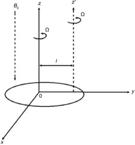
Consider the unsteady flow of an incompressible third grade fluid filling the semi-infinite space z > 0 above a disk at z =0. The disk is taken to be porous and non-conducting. Both cases of suction and injection/blowing are to be analyzed. The flow is generated by eccentric rotations of variable accelerated disk and third grade fluid at infinity. The disk and the fluid at infinity initially rotate about z'-axis with angular velocity Ω (see Figure 1). At t = 0, the disk suddenly starts rotating about z-axis with same angular velocity Ω and moving linearly with variable acceleration along x-axis. However, the fluid at t = 0 continues to rotate about the z'-axis. The axes of rotation of the disk and fluid at infinity are taken in the plane x = 0. The distance between the axes of rotations is denoted by l. The fluid is electrically conducting and a constant magnetic field B0 is applied in the transverse direction. We consider a slip between the velocity of the fluid at the surface of the disk and the velocity of the disk. The relative velocity between the fluid and the wall is assumed to be proportional to the shear rate at the wall.
The Cauchy stress tensor T (Fosdick and Rajagopal [27]) for a thermodynam-ically compatible third grade fluid is given by
( )
2 2
1 1 2 2 1 3 1 1
p
µ
α
α
β
tr= − + + + +
T I A A A A A (1)
in which p is the hydrostatic pressure, µ is the dynamic viscosity of the fluid. The equations governing the present flow are
0,
DOI: 10.4236/ojfd.2017.74033 487 Open Journal of Fluid Dynamics
Figure 1. Geometry of problem.
2 0 ,
D
B Dt
ρ V = ∇ ⋅ −T σ V (3) where ρ is the density and σ is the electrical conductivity of the fluid.
The velocity field V = u v w, , for our problem is given by
( )
, ,( )
, , 0u= −Ω +y f z t v= Ω +x g z t w= −W (4) satisfying the equation of continuity (2) identically. Here W0 > 0 denotes the suction and W0 < 0 the injection velocity.
The initial and boundary conditions of the problem are given by
2
1 xz 0 , 1 yz , at 0; for 0,
u−λτ = −Ω +y c t v−λτ = Ωx z= t> (5)
(
)
,
, as
, for all ,
u
= −Ω −
y l
v
= Ω
x
z
→ ∞
t
(6)(
)
, , for 0, and at 0,u= −Ω −y l v= Ωx z> t= (7)
where λ1 is a slip parameter, c0 is a constant having dimension L/T3 and the shear stresses are
2 2
1 2
2 3 2
3
2
2
xz
u u u v u v v
w
z t z z z y x z
u v u u u v
y x z z z z
τ
µ
α
β
∂ ∂ ∂ ∂ ∂ ∂ ∂
= + + + +
∂ ∂ ∂ ∂ ∂ ∂ ∂ ∂
∂ ∂ ∂ ∂ ∂ ∂
+ + + +
∂ ∂ ∂ ∂ ∂ ∂
(8)
2 2
1 2
2 3 2
3
2
2
yz
v v v u u u v
w
z t z z y z z x
u v v v v u
y x z z z z
τ
µ
α
β
∂ ∂ ∂ ∂ ∂ ∂ ∂
= + + + +
∂ ∂ ∂ ∂ ∂ ∂ ∂ ∂
∂ ∂ ∂ ∂ ∂ ∂
+ + + +
∂ ∂ ∂ ∂ ∂ ∂
DOI: 10.4236/ojfd.2017.74033 488 Open Journal of Fluid Dynamics Substituting (4) into (3), gives
( )
2
2 2
0 2 0
2 2
3 3 2
3 1
0
2 3 2
1
,
2
,
P f f f
x g W B f z t y
x z t z
f f g f f g
W
z z z z
t z z z
σ ν ρ ρ β α ρ ρ ∂ ∂ ∂ ∂
= Ω + Ω + − + − − Ω
∂ ∂ ∂ ∂
∂ ∂ ∂ ∂ ∂ ∂ ∂ + ∂ ∂ − ∂ + Ω∂ + ∂ ∂ ∂ +∂
(10)
( )
2 2 20 2 0
2 2
3 3 2
3 1
0
2 3 2
1
,
2
,
P g g g
y f W B g z t x
y z t z
g g f g f g
W
z z z z
t z z z
σ ν ρ ρ β α ρ ρ ∂ ∂ ∂ ∂
= Ω − Ω + − + − + Ω
∂ ∂ ∂ ∂
∂ ∂ ∂ ∂ ∂ ∂ ∂ + ∂ ∂ − ∂ − Ω∂ + ∂ ∂ ∂ +∂
(11) 2 0 0 1 , P B W z
σ
ρ
ρ
∂ =∂ (12)
where the modified pressure P is expressed as
(
2 1 2)
2 2 .f g
P p
z z
α α ∂ ∂
= − + ∂ +∂
(13)
Equation (12) shows that P is not a function of z. We can eliminate P from Equations (10)-(11) by differentiating and then integrating with respect to z, and combining the resulting equations to obtain the following equation
3 * 3 * 2 * *
1 0
1 1
0
2 3 2
2 2 * * * * 0 3 2 0, W
F F F F
i W
z
t z z z
B
F F F
i F
t z z z
α
α ν α
ρ ρ ρ
σ β
ρ
Ω
∂ − ∂ + − ∂ + ∂ ∂ ∂ ∂ ∂ ∂ ∂ ∂ ∂ ∂
− − Ω + + =
∂ Ω ∂ ∂ ∂
(14)
( )
* 2 * 2 * ** 2 1 0
0 1 2
2 * * 3 0, 2 , W
F F F F
F t c t l i
z t z z z
F F z z
α
λ
ρν
β
ρ
ν
∂ ∂ ∂ ∂ = Ω − Ω + + − −
∂ ∂ ∂ Ω ∂ ∂
∂ ∂ + ∂ ∂
Ω
(15)
( )
( )
* *
, 0, , 0 0,
F ∞t = F z = (16)
where
( )
( )
( )
*
, , , .
F z t = f z t +ig z t − Ωl (17)
Equation (15) together with the Conditions (16) and (17), in dimensionless variables, can be expressed as
(
)
(
)
3 3 2
2 3 2
2
1 2 2
2 0,
F F F F F
S i S
F F
i N F
α α α
η τ
τ η η η
β
η η η
∂ ∂ ∂ ∂ ∂ − + − + − ∂ ∂ ∂ ∂ ∂ ∂ ∂ ∂ ∂ − + + = ∂ ∂ ∂ (18)
( )
2 2 2 23 2
0, 1 F F F F F F ,
F τ cτ λ α S i β
η τ η η η η η
∂ ∂ ∂ ∂ ∂ ∂
= − + ∂ + ∂ ∂ − ∂ − ∂ + ∂ ∂
DOI: 10.4236/ojfd.2017.74033 489 Open Journal of Fluid Dynamics
(
,)
0,( )
, 0 0,F ∞
τ
= Fη
= (20)where
0
2 3 2
0 1 3 0
1 2 2 , , , , 2 2 , , , , . w F
F S z t
l
B l c
N c
l
η τ
ν ν
σ α α β β λ λ
ρ ρν ρν ν
∗ Ω
= = = = Ω
Ω Ω Ω Ω Ω = = = = = Ω Ω (21)
3. Numerical Solution
We obtain a numerical solution of the problem given by the governing Equation (18) together with Conditions (19)-(21). The discretized form of Equation (18) is presented using a finite difference scheme in ref. [19]. However, the boundary Condition (19) is discretized as
2 2
0,j 1 1,j 2 2,j 3 0,j1 1,j1 4 j 1
F =r F +r F +r F − −F − +r BT +cj k − (22)
where
(
)
(
)
[
]
[
]
(
) (
)
2 0 1 0 2 0 3 0 2 4 0 21, 0, 1, 0,
3
1 ,
1 2 ,
,
,
,
.
j j j j j
r h k i hk h S k
r i hk h S k r
r S k r
r h r
r h k r
BT F F F F
h
λ α αλ α λ
λ α αλ α λ
α λ αλ βλ = + − + + = − + + = − = = = − − (23)
To evaluate F0,j+1, we firstly take BTj+1=BTj in the system of algebraic
eq-uations and the solution of the system is sought which results in known values of
, 1; 1, 2, 3, , 1
i j
F + i= M − . Secondly, we update F0,j+1 by using iterative method
as follows:
(
)
(
)
(
)
1
0, 1 1 1, 1 2 2, 1 3 0, 1,
2
1, 1 0, 1
4 3 1, 1 0, 1
2 2
4 1 1 ,
k k
j j j j j
k k
j j
j j
F r F r F r F F
r F F F F
h
r c j k
βλ + + + + + + + + = + + − + − − + + − (24) where 0
0,j1 0,j1
F + =F + (25) and this iterative procedure is continued until 1
0, 1 0, 1
k k
j j
F ++ ≈F + . Furthermore, F0,0 is evaluated by letting F0, 1− =F1, 1− =0 and by using iterative method as
de-scribed above with 0 0,0 0
F = as initial guess.
For i=1, i=2, 3≤ ≤i M−3, i=M−2 and i=M−1, we respectively have
1 1,j 1 1 2,j 1 1 3,j1 1,
C F′ + +D F′ + +E F′ + =G′ (26)
2 1,j1 2 2,j1 2 3,j1 2 4,j1 2,
DOI: 10.4236/ojfd.2017.74033 490 Open Journal of Fluid Dynamics
2, 1 1, 1 , 1 1, 1 2, 1
i i j i i j i i j i i j i i j i
A F− + +B F− + +C F + +D F+ + +E F+ + =G (28)
2 4, 1 2 3, 1 2 2, 1 2 1, 1 2,
M M j M M j M M j M M j M
A − F − + +B − F − + +C − F − + +D − F − + =G′− (29)
1 3, 1 1 2, 1 1 1, 1 1,
M M j M M j M M j M
A −F − + +B −F − + +C −F − + =G′− (30)
where A B C D E G C D E B C Gi, i, i, i, i, i, 1′ ′ ′ ′ ′ ′, 1, 1, 2, 2, M−2 and GM′−1 are given in ref. [2]
and
(
)
(
)
(
(
)
)
(
)
(
(
)
)
2 2
1 1 1 0 1 3 0, 1, 4 1
2 2
2 2 2 3 0, 1, 4 1
1 1 ,
1 1 .
j j j
j j j
G G A L B r F F r BT c j k
G G A r F F r BT c j k
+ + ′ = − + − + + + − ′ = − − + + + −
In matrix form, the above set of M-1equationscan be finally written as
1 1 1 1
2 2 2 2 2
3 3 3 3 3 3
3 3 3 3 3 3
2 2 2 2
1 1 1
0 0 0 0 0 . . 0
0 0 0 0 . . 0
0 0 0 . . 0
. . . .
0 . 0 0 . 0
. . . .
0 0 0 . . 0
0 0 0 0 . . 0
0 0 0 0 0 . . 0
i i i i i i
M M M M M M
M M M M
M M M
C D E F
B C D E F
A B C D E F
A B C D E F
A B C D E F
A B C D F
A B C
− − − − − − − − − − − − − ′ ′ ′ ′ ′ 1 2 3 3 2 2 1 1 . . i M M M M M G G G G G G F G − − − − − ′ ′ = ′ ′ (31)
4. Discussion
[image:6.595.190.542.47.391.2] [image:6.595.56.540.556.728.2]Recalling that we have introduced the new features of the slip boundary condi-tion and the variable acceleracondi-tion of the disc in non-coaxial rotacondi-tion; we will lay emphasis to investigate the variation of slip parameter λ and the acceleration parameter c on the velocity profiles. However, for completeness we will show the variations of other parameters as well to look for the joint effects of already dis-cussed and the new phenomena. Firstly, in order to ensure reliability of our nu-merical scheme; the nunu-merical and the analytical results [20] are compared in Table 1, showing a good agreement.
Table 1.τ = 1, α = 0.1, β = 0, c = 1, S = 0.5, N = 0.5.
Η
Velocity profile f/Ωl Velocity profile g/Ωl
Analytic solution of
Khalid et al. [13] Present numerical solution Error Analytic solution of Khalid et al. [13] Present numerical solution Error
0.1 0.86939 0.86260 0.00679 −0.03230 −0.03116 0.00114
0.5 0.48638 0.46741 0.01897 −0.08579 −0.08224 0.00355
1.0 0.22426 0.20770 0.01656 −0.07167 −0.07192 0.00025
1.5 0.09681 0.08813 0.00868 −0.03882 −0.04580 0.00698
2.0 0.03783 0.03581 0.00202 −0.01405 −0.02523 0.01118
2.5 0.01250 0.01396 0.00146 −0.00148 −0.01270 0.01122
DOI: 10.4236/ojfd.2017.74033 491 Open Journal of Fluid Dynamics
[image:7.595.211.536.316.480.2]4.1. Variation of Slip Parameter
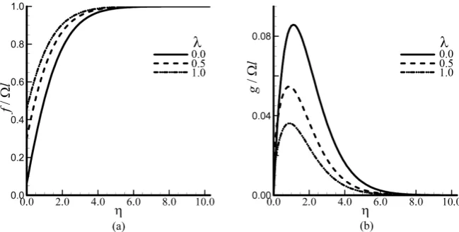
Figure 2 and Figure 3 show the effects of slip parameter λ on the flow pattern when
α
=0.2,β =
1.0
, c=0.25, S= =N 0 forτ
=0.5 andτ
=1.5. We note that increasing in λ enhances the velocity profile f/Ωl; whereas the velocity profile f/Ωl increases close to the disk and decreases away from the disk. It is further observed that the slip reduces the boundary layer thickness for the two velocity profiles. Thus the slip condition helps to control the boundary layer for rotating disc.4.2. Variation of Acceleration Parameter
Figure 4(a) reveals that the velocity profile f/Ωl increases with small increase in acceleration parameter c keeping the values of the parameters
α
=0.2,1.0
[image:7.595.211.534.526.692.2]β =
,λ
=0.5, S= =N 0 andτ
=1.5 fixed. However, for larger values of acceleration parameter; it is decreasing close to the disk and increasing away from the disk. The boundary layer thickness for the velocity profile f/Ωl decreasesFigure 2. Velocity profiles against distance from the disk for different values of the slip
parameter λ when α = 0.2, β = 1.0, c = 0.25, S = N = 0 and τ = 0.5.
Figure 3. Velocity profiles against distance from the disk for different values of the slip
DOI: 10.4236/ojfd.2017.74033 492 Open Journal of Fluid Dynamics
Figure 4. Velocity profiles against distance from the disk for different values of the
acce-leration c when α = 0.2, β = 1.0, λ = 0.5, S = N = 0 and τ = 1.5.
with c. Furthermore, it is evident from Figure 4(b) that the velocity profile g/Ωl increases with increasing c close to the disk while it decreases away from the disk. The momentum boundary layer thickness for the velocity profile g/Ωl, de-creases with increasing c.
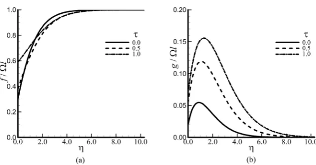
4.3. Time Evolution of the Velocity Field
The evolution of the velocity profiles f/Ωl and g/Ωl for different values of time parameter τ in the case of rigid plate and non-conducting third grade fluid
β
, are shown in Figure 5. Here we takeα
=0.2,β =
1.0
, c=0.25 and0.5
λ
= . This leads us to believe that; as the time evolves, the velocity profilef/Ωl increases close to the disk and decreases nominally farther from the disk. We note from Figure 5(a) that thickness of the boundary layer increases as the time
τ
progresses. It is evident from Figure 5(b) that the velocity profile g/Ωl and thickness of the boundary layer are increasing with timeτ
.4.4. Variation of Other Physical Parameters
Figure 6 is drawn to examine the behavior of third grade parameter
β
when 0.2α
= , c=0.25,λ
= =S N=0 andτ
=0.5. It is observed from Figure6(a) that an increase in
β
slightly reduces the velocity profile f/Ωl and a slight increase in the thickness of boundary layer. The behavior is reversed for the ve-locity profile g/Ωl but a slight increase in the thickness of boundary layer is seen from Figure 6(b). However, in the presence of slip parameter λ = 0.25, we refer to Figure 7. This Fig. shows that there is slight increase in the velocity profiles f/Ωl and g/Ωl at the surface of the disk due to the presence of the slip parameter; otherwise the behavior is almost the same as has been seen in Figure 6.The effects of injection/suction can be seen from Figure 8. The fluid velocities f/Ωl and g/Ωl are found to increase and decrease respectively at the surface of the disk; for slip parameter
λ
=0.5, magnetic parameter N=0 forα
=0.2,1.0
DOI: 10.4236/ojfd.2017.74033 493 Open Journal of Fluid Dynamics
Figure 5. Velocity profiles against distance from the disk for different values of time τ
[image:9.595.211.534.282.443.2]when α = 0.2, β = 1.0, c = 0.25, λ = 0.5 and S = N = 0.
Figure 6. Velocity profiles against distance from the disk for different values of the third
grade parameter β when α = 0.2, c = 0.25, λ = S = N = 0 and τ = 0.5.
Figure 7. Velocity profiles against distance from the disk for different values of the third
grade parameter β when α = 0.2, c = 0.25, λ = 0.25, S = N = 0 and τ = 0.5.
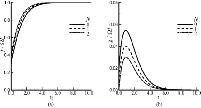
[image:9.595.211.535.489.650.2]DOI: 10.4236/ojfd.2017.74033 494 Open Journal of Fluid Dynamics effects of magnetic field parameter N are identical to that of suction (see Figure 9).
To see the effects of rotation Ω; we draw the Figure 10 and Figure 11 in the absence and presence of the slip parameter λ when
α
=0.2,β =
1.0
, c=1,0
S= =N , l=0.25 and
τ
=1.5. It is found that increasing rotation Ω the ve-locity profile f/Ωl increases whereas g/Ωl decreases. Moreover the velocity pro-file f/Ωl becomes stable at some values of Ω. It is further noticed that in the presence of the slip parameterλ
=0.25 both velocity profiles f/Ωl and g/Ωl decrease at the surface of the disk as compared to the absence of slip parameter0
[image:10.595.211.532.298.473.2] [image:10.595.212.535.519.692.2]λ
= . Otherwise, the behaviours of both f/Ωl and g/Ωl are the same as shown in Figure 10 and Figure 11. Remembering that this problem is essentially a three dimensional; three dimensional velocity profiles are plotted in Figures 12-16. These streamlines are drawn by taking into consideration various physical pa-rameters mentioned in Figure captions.Figure 8. Velocity profiles against distance from the disk for different values of porosity S
when α = 0.2, β = 1.0, c = 0.25, λ = 0.5, N = 0 and τ = 0.5.
Figure 9. Velocity profiles against distance from the disk for different values of the
DOI: 10.4236/ojfd.2017.74033 495 Open Journal of Fluid Dynamics
Figure 10. Velocity profiles against distance from the disk for different values of the
[image:11.595.212.534.285.446.2]rota-tion parameter Ω when α = 0.2, β = 1.0, c = 1, λ = S = N = 0, l2 = 0.25 and τ = 1.5.
Figure 11. Velocity profiles against distance from the disk for different values of the
rota-tion parameter Ω when α = 0.2, β = 1.0, c = 1, λ = 0.25, S = N = 0, l2 = 0.25 and τ = 1.5.
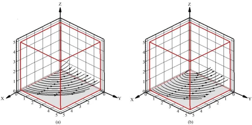
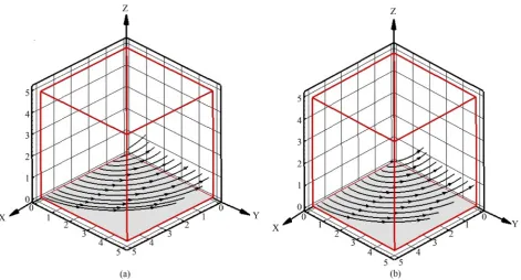
[image:11.595.109.539.493.706.2]DOI: 10.4236/ojfd.2017.74033 496 Open Journal of Fluid Dynamics Figure 13. Streams lines for (a) λ = 0 and (b) λ = 1.0 when α = 0.2, β = 1.0, c = 1.0, τ = 0.75, S = 0.5 and N = 0.
Figure 14. Streams lines for (a) c = 0 and (b) c = 1.0 when α = 0.2, β = 1.0, λ = 1.0, τ = 1.25, S = 0.5 and N = 0.
5. Conclusion
[image:12.595.63.535.344.598.2]DOI: 10.4236/ojfd.2017.74033 497 Open Journal of Fluid Dynamics Figure 15. Streams lines for (a) S = 0 and (b) S = 1.0 when α = 0.2, β = 1.0, λ = 1.0, τ = 1.25, S = 0.5, N = 0 and c = 1.
Figure 16. Streams lines for (a) N = 0 and (b) N = 2.0 when α = 0.2, β = 1.0, λ = 1.0, τ = 0.75, S = 1.0 and c = 1.
[image:13.595.67.535.341.574.2]DOI: 10.4236/ojfd.2017.74033 498 Open Journal of Fluid Dynamics The effects of these quantities on g/Ωl are exactly the opposite. The effects of suction and injuction/blowing on the boundary layer thickness remain the same irrespective of third grade fluid and the slip condition. That is, the suction causes thinning and blowing causes thickening of the boundary layer thickness. We remember that the magnetic field is applied parallel to the axis of rotation. This causes a decrease in the thickness of boundary layer for f/Ωl and an increase for the velocity profile g/Ωl. The comparison of the velocity profile for variable ac-celeration with constant acac-celeration of the disc discussed earlier [2] reveals im-portant observation. For time τ < 1, the velocity profiles for constant accelerated flow are greater than that of variable accelerated flow. However, for the time τ > 1, the velocity profiles for variable accelerated flow are much larger than con-stant accelerated flow.
Acknowledgements
This project was funded by the Deanship of Scientific Research (DSR), King Abdulaziz University, under grant No. (41-130-35-HiCi). The author, therefore, acknowledge technical and financial support of KAU.
References
[1] Erdogan, M.E. (1997) Unsteady Flow of a Viscous Fluid Due to Non-Coaxial Rota-tions of a Disk and a Fluid at Infinity. International Journal of Non-Linear Me-chanics, 32, 285-290. https://doi.org/10.1016/S0020-7462(96)00065-0
[2] Bhattacharyya, K. (2011) Effects of Heat Source/Sink on MHD Flow and Heat Transfer over a Shrinking Sheet with Mass Suction. Chemical Engineering Research Bulletin, 15, 12-17. https://doi.org/10.3329/cerb.v15i1.6524
[3] Bhattacharyya, K., Arif, M.G. and Ali, W.P. (2012) MHD Boundary Layer Stagna-tion-Point Flow and Mass Transfer over a Permeable Shrinking Sheet with Suc-tion/Blowing and Chemical Reaction. ActaTechnica, 57, 1-15.
[4] Bhattacharyya, K., Mukhopadhyay, S. and Layek, G.C. (2012) Reactive Solute Transfer in Magnetohydrodynamic Boundary Layer Stagnation-Point Flow over a Stretching Sheet with Suction/Blowing. Journal Chemical Engineering Communica-tions, 199, 368-383.https://doi.org/10.1080/00986445.2011.592444
[5] Bhattacharyya, K. and Pop, I. (2011) MHD Boundary Layer Flow Due to an Expo-nentially Shrinking Sheet. Magnetohydrodynamics, 47, 337-344.
[6] Hayat, T., Ellahi, R. and Asghar, S. (2004) Unsteady Periodic Flows of a Magneto-hydrodynamic Fluid Due to Noncoaxial Rotations of a Porous Disk and a Fluid at Infinity. Mathematical and Computer Modelling, 40, 173-179.
https://doi.org/10.1016/j.mcm.2003.09.035
[7] Hayat, T., Zamurad, M., Asghar, S. and Siddiqui, A.M. (2003) Magnetohydrody-namic Flow Due to Non-Coaxial Rotations of a Porous Oscillating Disk and a Fluid at Infinity. International Journal of Engineering Science, 41, 1177-1196.
https://doi.org/10.1016/S0020-7225(03)00004-1
[8] Hayat, T., Haroon, T., Asghar, S. and Siddiqui, A.M. (2001) Unsteady MHD Flow Due to Non-Coaxial Rotations of a Porous Disk and a Fluid at Infinity. Acta Me-chanica, 151, 127-134. https://doi.org/10.1007/BF01272530
DOI: 10.4236/ojfd.2017.74033 499 Open Journal of Fluid Dynamics Non-Torsional Oscillations and a Fluid Rotating at Infinity. International Journal of Engineering Science, 38, 175-196. https://doi.org/10.1016/S0020-7225(99)00017-8 [10] Fetecau, C., Awan, U. and Athar, M. (2010) A Note on “Taylor-Couette Flow of a
Generalized Second Grade Fluid Due to a Constant Couple”. Nonlinear Analysis: Modelling and Control, 15, 155-158.
[11] Hayat, T., Mustafa, M. and Hendi, A.A. (2011) Time-Dependent Three-Dimensional Flow and Mass Transfer of Elastico-Viscous Fluid over Unsteady Stretching Sheet. Applied Mathematics and Mechanics, 32, 167-178.
https://doi.org/10.1007/s10483-011-1403-7
[12] Narain, R. and Kara, A.H. (2010) An Analysis of the Conservation Laws for Certain Third-Grade Fluids. Nonlinear Analysis: Real World Applications, 11, 3236-3241. https://doi.org/10.1016/j.nonrwa.2009.11.018
[13] Niu, J., Fu, C. and Tan, W.C. (2010) Stability of Thermal Convection of an Ol-droyd-B Fluid in a Porous Medium with Newtonian Heating. Physics Letters A, 374, 4607-4613. https://doi.org/10.1016/j.physleta.2010.09.028
[14] Rajagopal, K.R. (1992) Flow of a Viscoelastic Fluid between Rotating Disks. Theo-retical and Computational Fluid Dynamics, 3, 185-206.
https://doi.org/10.1007/BF00417912
[15] Rivlin, R.S. and Ericksen, J.L. (1955) Stress Deformation Relations for Isotropic Materials. Archive for Rational Mechanics and Analysis, 4, 323-425.
[16] Vieru, D., Fetecau, C. and Sohail, A. (2011) Flow Due to a Plate That Applies an Accelerated Shear to a Second Grade Fluid between Two Parallel Walls Perpendi-cular to the Plate. Zeitschrift für angewandte Mathematik und Physik, 62, 161-172. https://doi.org/10.1007/s00033-010-0073-4
[17] Siddiqui, A.M., Haroon, T., Hayat, T. and Asghar, S. (2001) Unsteady MHD Flow of a Non-Newtonian Fluid Due to Ecentric Rotation of a Porous Disk and a Fluid at Infinity. Acta Mechanica, 147, 99-109. https://doi.org/10.1007/BF01182355
[18] Hayat, T., Haroon, T., Asghar, S. and Siddiqui, A.M. (2003) MHD Flow of a Third-Grade Fluid Due to Eccentric Rotations of a Porous Disk and a Fluid at In-finity. International Journal of Non-Linear Mechanics, 38, 501-511.
https://doi.org/10.1016/S0020-7462(01)00075-0
[19] Asghar, S., Hanif, K. and Hayat, T. (2010) Flow of a Third Grade Fluid Due to an Accelerated Disk. International Journal for Numerical Methods in Fluids, 63, 887-902.
[20] Asghar, S., Hanif, K., Hayat, T. and Khalique, C.M. (2007) MHD Non-Newtonian Flow Due to Non-Coaxial Rotations of an Accelerated Disk and a Fluid at Infinity. Communications in Nonlinear Science and Numerical Simulation, 12, 465-485.
https://doi.org/10.1016/j.cnsns.2005.04.006
[21] Bhattacharyya, K. (2012) Slip Effects on Boundary Layer Flow and Mass Transfer with Chemical Reaction over a Permeable Flat Plate in a Porous Medium. Frontiers in Heat and Mass Transfer, 3, Article ID: 043006.
[22] Bhattacharyya, K., Layek, G.C. and Gorla, R.S.R. (2012) Slip Effect on Boundary Layer Flow on a Moving Flat Plate in a Parallel Free Stream. International Journal of Fluid Mechanics Research, 39, 438-447.
https://doi.org/10.1615/InterJFluidMechRes.v39.i5.50
DOI: 10.4236/ojfd.2017.74033 500 Open Journal of Fluid Dynamics https://doi.org/10.1088/0256-307X/28/9/094702
[24] Bhattacharyya, K., Mukhopadhyay, S. and Layek, G.C. (2011) Steady Boundary Layer Slip Flow and Heat Transfer over a Flat Porous Plate Embedded in a Porous Media. Journal of Petroleum Science and Engineering, 78, 304-309.
https://doi.org/10.1016/j.petrol.2011.06.009
[25] Bhattacharyya, K., Vajravelu, K. and Hayat, T. (2013) Slip Effects on the Parametric space and the Solution for Boundary Layer Flow of Casson Fluid over a Porous Stretching/Shrinking Sheet. International Journal of Fluid Mechanics Research, 40, 482-493.https://doi.org/10.1615/InterJFluidMechRes.v40.i6.20
[26] Ebaid, A. (2008) Effects of Magnetic Field and Wall Slip Conditions on the Peristal-tic Transport of a Newtonian Fluid in an Asymmetric Channel. Physics Letters A, 372, 4493-4499.https://doi.org/10.1016/j.physleta.2008.04.031
[27] Fosdick, R.L. and Rajagopal, K.R. (1980) Thermodynamics and Stability of Fluids of Third Grade. Proceedings of the Royal Society of London, 369, 351-377.