Forecasting national recessions using state level data

Munich Personal RePEc Archive

Forecasting national recessions using

state-level data

Owyang, Michael T. and Piger, Jeremy and Wall, Howard J.

Federal Reserve Bank of St. Louis, University of Oregon, CEE,

Lindenwood University

10 April 2012

Online at

https://mpra.ub.uni-muenchen.de/57716/

Forecasting National Recessions Using State Level Data

∗

Michael T. Owyang

Jeremy Piger

Howard J. Wall

This draft: July 23, 2014

Abstract: A large literature studies the information contained in national-level economic indicators, such as financial and aggregate economic activity variables, for forecasting and nowcasting U.S. business cycle phases (expansions and recessions.) In this paper, we in-vestigate whether there is additional information useful for identifying business cycle phases contained in subnational measures of economic activity. Using a probit model to forecast the NBER expansion and recession classification, we assess the incremental information content of state-level employment growth over a commonly used set of national-level predictors. As state-level data adds a large number of predictors to the model, we employ a Bayesian model averaging procedure to construct forecasts. Based on a variety of forecast evaluation metrics, we find that including state-level employment growth substantially improves nowcasts and very short-horizon forecasts of the business cycle phase. The gains in forecast accuracy are concentrated during months of national recession.

Keywords: turning points, probit, Bayesian model averaging, nowcasting

JEL Classification Numbers: C52, C53, E32, E37

∗_{We thank the editor, two anonymous referees, and seminar participants at the University of Houston,}

Federal Reserve Bank of St. Louis, and University of Texas, El Paso for helpful comments. This paper also benefited from conversations with Graham Elliott and Oscar Jord´a. Kristie M. Engemann and Kate Vermann provided research assistance. The views expressed herein do not reflect the official positions of the Federal Reserve Bank of St. Louis or the Federal Reserve System.

†_{Research Division, Federal Reserve Bank of St. Louis, ([email protected])} ‡_{Department of Economics, University of Oregon, ([email protected])}

1

Introduction

A traditional view of the U.S. business cycle is that of alternating phases of expansion

and recession, where expansions correspond to widespread, persistent growth in economic

activity, and recessions consist of widespread, relatively rapid, decline in economic activity.1

A large literature investigates different aspects of these business cycle phases and documents

asymmetries across them. Such work experienced a resurgence following Hamilton (1989),

who built a modern statistical model of the alternating phases characterization of the business

cycle by describing the latent business cycle phase as following a first-order Markov process

that influences the mean growth rate of output.

Timely identification of business cycle phases, and the associated turning points between

them, is of particular interest to academics, policymakers, and practitioners. A substantial

literature has investigated the extent to which the business cycle phase can be predicted

using a variety of economic and financial time series.2 _{Here, the forecasting problem is to}

use data available at time period t to predict whether period t+h will be an expansion or recession period. The most ambitious task is of course to predict the future business cycle

phase at long horizons, and the literature has had some limited success predicting recessions

one-year ahead by using information on the slope of the yield curve. For forecasting the

business cycle phase at short horizons, predictors measuring aggregate real activity, such as

employment or output growth, are found to be valuable. Not surprisingly, this is especially

true for h= 0 predictions, which are typically referred to as “nowcasts.”3

Although they have received less attention in the literature, short-horizon forecasts and

nowcasts of business cycle turning points are of considerable interest. While long horizon

forecasts of the business cycle phase would give economic agents the most advance warning

1_{See Mitchell (1927) and Burns and Mitchell (1946).}

2_{See e.g., Estrella (1997), Estrella and Mishkin (1998), Kauppi and Saikkonen (2008), Rudebusch and}

Williams (1991) and Berge (2013). For a recent summary of this literature, see Katayama (2008).

3_{Here, the prefix “now” in nowcast refers to the use of data available in periodtto evaluate whether period} t_{is a recession or expansion period. Note that because of data reporting lags, most of the data available in}

of a new business cycle turning point, it has historically been the case that new business

cycle phases have not been forecasted accurately. Indeed, in most cases new phases have

only been identified in real time after many months have passed following the turning point.4

As a recent example of this, Hamilton (2011) surveys a wide range of statistical models that

were in place to nowcast business cycle turning points using aggregate data, and finds that

such models did not send a definitive signal regarding the December 2007 NBER peak until

late 2008. Improved short-horizon forecasts and nowcasts thus hold the promise of giving a

quicker signal that a new recession or expansion is imminent or has already begun. These

could improve the speed of both policy and private sector adjustments to this new business

cycle phase.

The existing literature has focused on the use of predictors measured at the national

level. However, there is reason to believe that variables measured at the subnational level

would be useful for identifying the national business cycle phase. Owyang et al. (2005) and

Hamilton and Owyang (2011) provide evidence that the business cycles of individual U.S.

states are often out of phase with that of the nation. If these phase shifts are systematic, then

incorporating data from leading regions may be useful for predicting the national business

cycle phase. Also, even if subnational regions are coincident with the aggregate business cycle

phase, there may be regions that experience recession and expansion phases more severely

than the nation as a whole. In these cases, incorporating data from these regions will provide

a stronger signal regarding the business cycle phase that is currently in operation, and will

thus improve nowcasts and short-horizon forecasts of the business cycle phase.5

In this paper, we assess whether state-level economic indicators contain incremental

in-formation useful for forecasting and nowcasting U.S. business cycle phases. Following the

4_{Since the inception of the NBER’s business cycle dating committee in 1978, the NBER has announced new}

business cycle peaks with a lag of 7.5 months and troughs with a lag of 15 months. Chauvet and Piger (2008) show that statistical models estimated using aggregate data improve on the NBERs timeliness for troughs, but not for peaks.

5_{Short-horizon forecasts will be improved because of the persistence of business cycle phases. If subnational}

bulk of the literature, we take the NBER’s chronology of the dates of U.S. business cycle

phases as given. We then construct a monthly probit model to attach probabilities of

ex-pansion and recession to current and future periods, which incorporates both national- and

state-level variables as predictors. The national variables we use are those found to be good

predictors of the national business cycle phase at various horizons by the existing literature.

In particular, we focus on interest rates, asset prices, aggregate employment, and

aggre-gate industrial production. To these, we add state-level employment growth to capture the

predictive ability of subnational economic activity measures.

By using state-level employment growth, we measure subnational economic activity with

a coincident indicator, rather than a leading indicator. This raises the question of what

hope such data would have for helping predict the aggregate business cycle phase? While

state employment growth is a coincident indicator, it is likely an indicator that is coincident

with that state’s business cycle phase. Thus, as discussed above, if a state’s business cycle

leads the national business cycle phase, then state employment growth could be a leading

indicator for the national business cycle phase. As evidence of this, Hernandez-Murillo

and Owyang (2006) show that adding regional employment data can assist in predicting

aggregate employment growth in the United States. Also, even if state employment growth

is coincident with the national level business cycle phase, state employment growth may

provide improved nowcasts and short-horizon forecasts of the aggregate business cycle phase

if the employment response to the business cycle phase in operation is relatively strong for

certain states.6

Despite the potential promise of state-level data for improving nowcasts and forecasts of

6_{Our choice to focus on state-level employment growth is also driven by the lack of suitable leading}

business cycle phases, simply adding this data into the information set used in a forecasting

model is problematic. It is likely that many states will not be informative about future

national business cycle phases at all, or perhaps any, forecast horizons. Further, there is

significant collinearity in employment growth across U.S. states. Put together, the naive

use of all state-level data will likely lead to an overparameterized model with a high level

of estimation uncertainty, which will not bode well for improved forecasting performance.

One may reduce, though not eliminate, these problems by aggregating across states to the

regional level. However, this aggregation would potentially average states that contain very

different forecasting information.

In this paper, we take a Bayesian model averaging (BMA) approach to incorporate

state-level predictors in a forecasting model. In particular, we explicitly incorporate the selection of

predictors into the estimation of the model, and average forecasts across models with different

sets of predictors by constructing the posterior predictive distribution for the future business

cycle phase. This approach allows individual states with predictive content for the business

cycle phase at a particular horizon to be highlighted in producing forecasts, while pushing

out those states that are not informative. Notably, the Bayesian approach to constructing

forecasts also incorporates uncertainty regarding model parameters.

Based on a variety of forecast evaluation metrics, we find that including state-level

em-ployment growth significantly improves nowcasts and very short-horizon forecasts of the

NBER business cycle phase over those produced by a model using only national-level data.

We document the incremental information content of the state-level data based on the

model’s out-of-sample forecast performance over the past 30 years. We also show that the

forecasting improvement comes primarily from improved classification of recession months.

As an example, for one-month ahead forecasts, nearly a quarter of all recession months are

correctly classified using the model that includes state-level data, but not by the model based

on national-level data only. Also, again based on one-month ahead forecasts, the December

state and national-level data, as opposed to late July 2008 when using only national-level

data.

The balance of the paper is as follows: Section 2 outlines the empirical model used for

forecasting recessions and describes the Bayesian approach to estimation and construction of

forecasts. Section 3 describes the national- and state-level data used to estimate the model

and construct forecasts. Section 4 presents the evaluation of the out-of-sample forecasts.

Section 5 summarizes and concludes.

2

Empirical Approach

2.1

Model

Define S_t ∈ {0,1} as a binary random variable that indicates whether month t belongs to an expansion (0) or recession (1) phase. Our objective is to forecast St+h based on

information available to a forecaster at the end of month t. This information may include national-, state-, or regional-level variables and is collected in the n×1 vector Xt.

Following the bulk of the existing literature, we use a probit model to link St+h toXt:

Pr [St+h = 1|ρ] =Φ(α+Xt0β), (1)

where the link function, Φ(.), is the standard normal cumulative density function, β is an

n × 1 vector of coefficients, and ρ = [α,β0_]0 _{is an (n+ 1) ×1 vector holding the model}

parameters.

The number of potentially relevant forecasting variables available in Xt may be large.

This is especially true with the inclusion of subnational data, as variables are measured

repeatedly across regions or states. This is problematic from a forecasting perspective, as

it is well established that highly parameterized models tend to have poor out-of-sample

the predicitve probabilities are functions of the values of all the included variables. This

means that including irrelevant variables could bias the forecasts. Here, we focus on a

modified version of (1), in which not all variables in Xt need be included in the model. In

particular, define γ as an n ×1 vector of zeros and ones, with a one indicating that the corresponding variable inXtshould be included in the model. We rewrite (1) to incorporate

this variable selection as follows:

Pr [St+h = 1|ργ,γ] =Φ α+X 0

γ,tβγ , (2)

whereXγ,t,ργ, andβγ contain the elements ofXt,ρ, andβrelevant for the variables selected

byγ. As is described in the next subsection, we treat γ as unknown, and estimate its value

along with the parameters of the model using Bayesian techniques.

2.2

Estimation

To estimate the model in (2) we take a Bayesian approach, which has some key advantages

for our purposes. For one, uncertainty about which variables should be included in the model

– that is uncertainty about γ – can be formally incorporated into Bayesian estimation in

a straightforward manner. Related to this, the Bayesian framework provides a mechanism,

through the posterior predictive density, to obtain forecasts that average over different choices

for variable inclusion and the values of unknown parameters.

Bayesian estimation requires priors be placed on the model parameters, ργ, as well as

the covariate selection vector, γ. We specify diffuse, i.i.d., mean-zero normal distributions

for the individual parameters collected in ργ:

p(ργ) =N 0kγ+1,σ

2_I

kγ+1 ; σ

2 _{= 10, (3)}

where k_γ =γ0_{γ is the number of covariates selected by γ, 0}

kγ+1 is a (kγ+ 1)×1 vector of

distribution defined across the 2n _{different possible choices ofγ. LetN}

i = n_i be the number

of choices of γ for which kγ =i. The prior probability over γ is then:

Pr (γ)∝ 1

Nkγ

. (4)

This distribution is flat in two dimensions. First, it assigns equal probability to all choices

of γ that have the same k_γ. In other words, versions of (2) with the same number of covariates will receive equal prior probability. Second, the prior assigns equal cumulative

probability to groups of choices for γ that imply different numbers of covariates. That is,

Pr (kγ =i) = Pr (kγ=j), i, j = 0,1,· · ·, n.

7

To implement Bayesian estimation, we employ the Gibbs sampler to obtain draws from

the joint posterior distribution, π(ργ,γ|S

t_{), where S}t _{= [S}

h+1,· · ·, St]

0

represents the

ob-served data.8 _{The Gibbs sampler is facilitated by augmenting the system with a continuous}

variable yt that is deterministically related to the observed state variable St (Tanner and

Wong (1987)). Defineyt as:

yt=α+Xγ0,t hβγ+ut, (5)

where ut∼i.i.d.N(0,1). Given (2), the relationship between yt and St is:

St= 1 if yt≥0.

The Gibbs sampler is then implemented in two blocks. In the first, ργ and γ are sampled

conditional onStand the augmented datayt= [y_h+1,· · ·, y_t]0, as a draw from the conditional posterior distribution π(ργ,γ|y

t_,St_{). As S}t _{is fully determined by y}t_{, this distribution}

7_{Note that this prior does not assign equal probability to all possible choices of}

γ. While seemingly attractive

as a “flat” prior, an equal weights prior would give substantially different prior weight to the number of variables included. For example, if there are 50 possible variables, the cumulative prior probability of all models with 3 variables would be 16 times the cumulative prior probability of all models with 2 variables.

8_{See, for example, Albert and Chib (1993), Gelfand and Smith (1990), Casella and George (1992), and Carter}

simplifies toπ(ργ,γ|y

t_{). In the second, the augmented datay}t_{is sampled conditional onρ}

γ,

γ, and St_{, from the conditional posterior distribution π(y}t_|ρ

γ,γ,S

t_{). We now describe each}

of these blocks in detail:

Sampling π(ργ,γ|y

t₎

As suggested by Holmes and Held (2006), we jointly sample ργ and γ from:

π ργ,γ|y

t

=πρ ργ|γ,y

t

Pr γ|yt ,

by employing a Metropolis step. Given a previous draw of ργ and γ, denoted h

ρ[γg],γ[g] i

, we

obtain a candidate for the covariate selection vector, denoted γ⇤_{, by sampling a proposal}

distribution q γ⇤_|γ[g] _{. Conditional on γ}⇤_{, we then obtain a candidate for ρ}

γ, denoted ρ ⇤ γ,

by sampling from the full conditional posterior density πρ(ργ|γ ⇤_,yt_).

The proposal distribution q γ⇤_|γ[g] _{is set as follows. Conditional on γ}[g]_{, the candidate}

covariate selection vector γ⇤ _{is drawn with equal probability from the set of vectors that}

includes γ[g] _{and all other vectors that alter a single element of γ}[g] _{(either from 0 to 1 or}

1 to 0.) In other words, the candidate covariate selection vector will either select the same

covariates asγ[g]_{, take away one covariate fromγ}[g]_{, or add one covariate toγ}[g]_{. One notable}

property of this proposal distribution is that q(γ⇤_|γ[g]_{) will equal q(γ}[g]_|γ⇤_).

The full conditional distribution for ρ, πρ(ργ|γ

⇤_,yt_{), is as follows. Define X}

γ,t h = ⇥

1, X0 γ,t h

⇤

, t =h+ 1,· · ·, t and let X_γt h represent the (t−h)×(kγ+ 1) matrix of stacked

Xγ,t h. Then, given the prior distribution in (3), the conditional posterior forργ is:

πρ ργ|γ ⇤_,yt

∼N(mγ∗,M_γ∗),

Mγ∗ = ✓

1

σ2Ikγ+1+ (X

t h

γ )

0

Xt h_γ

◆ 1

,

mγ∗ =M_γ∗ (Xt h γ )

0

yt h .

The candidate, ρ⇤

γ is then sampled fromN(mγ∗,Mγ∗).

The Metropolis step assigns an acceptance probabilityAto determine whether or not the candidate will be accepted. Given the gth _drawh_ρ[g]

γ ,γ[g] i

, the (g+ 1)th draw is determined by:

⇥

ρ[_γg+1],γ[g+1]⇤=

8 > < > : ⇥ ρ⇤ γ,γ

⇤⇤ _{with probability A} h

ρ[γg],γ[

g]i _{with probability 1−A} ,

where:

A= min

⇢

1, Pr(γ

⇤ |yt₎

Pr(γ[g]_|yt₎ .

From Bayes’ Rule:

Pr(γ|yt)∝f(yt|γ) Pr(γ),

where f(yt_{|γ) is the marginal likelihood for the augmented data, y}t_{, conditional on the}

choice of variables γ, and Pr(γ) is the prior distribution over γ. We can then rewrite the

acceptance probability as:

A= min

⇢

1, f(y

t_|γ⇤

) Pr (γ⇤

)

f(yt_|γ[g]_{) Pr (γ}[g]₎ .

To computeA, we must computef(yt_{|γ). Given the prior distribution in (3), this is available}

f(yt|γ)∼N(0,_Σγ)

where Σγ =It h+σ

2_Xt h

γ (X

t h

γ )

0_{. Using the equation for the multivariate normal we then}

have:

A= min

8 < :1,

Σγ[g]

0.5

exp −0.5 (yt)0

(Σγ∗)

1

yt Pr (γ⇤)

|Σγ∗|

0.5

exp⇣−0.5⇣(yt)0

Σγ[g]

1

yt⌘⌘Pr γ[g]

9 =

;. (6)

Sampling π(yt|ργ,γ,S

t₎

Conditional on ργ and γ, yt is normally distributed with mean δγ,t and unit variance,

where:

δγ,t =α+X 0

γ,t hβγ.

However, the target distribution also conditions on St_{, which adds the requirement that the}

sign of yt must match the realization of St. In this case, yt has a truncated normal density:

yt ∼

8 > > < > > :

N(δγ,t,1)I[yt 0] if St = 1

N(δγ,t,1)I[yt<0] if St = 0

,

where the indicator I_[.] reflects the direction of the truncation. A draw from yt is then obtained by drawingytfrom the appropriate truncated normal distribution,t=h+ 1,· · ·, T.

Given arbitrary starting values for ργ and γ, the above two sampling steps are iterated

to obtain drawshρ[γg],γ[g] i

, forg = 1,· · ·, G. Following a suitably large initialization period, these draws will be from the joint posterior distribution, π(ργ,γ|S

t_{). In all estimations}

reported below, we sample 20,000 initialization draws to achieve convergence. Results are

initialization period by ensuring that results from two different runs of the Gibbs Sampler

with dispersed sets of starting values were similar.

2.3

Construction of Forecasts and Forecast Evaluation

To forecast the business cycle phase in period t+h, we use the posterior predictive

dis-tribution:

Pr⇥St+h = 1|St

⇤

. (7)

Although the posterior predictive distribution is not available analytically, we can simulate

from (7) as follows. The posterior predictive distribution is factored as:

Pr⇥St+h = 1|St

⇤ = Z ργ Z γ

Pr⇥St+h = 1|ργ,γ,S

t⇤_{π ρ}

γ,γ|S

t _d

γdργ. (8)

Equation (8) suggests a Monte Carlo integration approach to calculate the posterior

predic-tive distribution. Specifically, given a draw hρ[γg],γ[g] i

from π(ργ,γ|S

t_{) we simulate a value}

of St+h, denoted St+h[g], from:

Pr⇥S_t+h = 1|ρ[γg],γ

[g]_,St⇤

= Pr⇥S_t+h = 1|ρ[γg],γ

[g]⇤ ₌

Φ⇣α[g]+X0 γ[g],tβ

[g]

γ ⌘

,

where the validity of the first equality sign comes from the fact that, given the model in

(2) and the model parameters, the observed data St _{are not informative for the distribution}

of St+h. The simulated value S[ g]

t+h is a draw from the posterior predictive distribution,

Pr [St+h|St], and it follows that:

lim G!1 1 G G X g=1 ⇣

St+h[g]

⌘

= Pr[St+h = 1|St] (9)

as our (point) forecast of St+h. In the following, we refer to this forecast as Sbt+h. It is

worth emphasizing that Sbt+h is not conditional on model parameters or the choice of which

variables to include in the model. These sources of uncertainty have been integrated, over

their respective posterior distributions, out of the prediction. Note that the integration over

the posterior distribution for γ gives Sbt+h the interpretation of a BMA prediction.

To evaluateSb_t+h, we consider a variety of forecast evaluation metrics. The first is the Brier (1950) quadratic probability score (QP S), which is a probability analog of mean squared error:

QP S = 2

τ2−τ1

τ2 X

t+h=τ1+1 ⇣

b

St+h−St+h

⌘2 ,

whereτ1 andτ2 are chosen to cover the period over whichSbt+h is being evaluated. TheQP S

ranges from 0 to 2, with 0 indicating perfect forecast accuracy.

While the QP S is a standard metric for the evaluation of forecasts of binary variables, it does not directly evaluate Sbt+h as a classifier of St+h. Specifically, the QP S is focused

on the distance between Sbt+h and St+h, rather than on the ability of Sbt+h to classify St+h

accurately. This distinction is meaningful, as it is simple to construct examples where a

forecasting model with perfect classification ability has an inferiorQP S to a model with less than perfect classification ability.9 _{Thus, we also consider two forecast evaluation metrics}

that directly assess classification ability. The first is the correspondence, defined as the

proportion of months for which Sbt+h correctly indicates the NBER business cycle phase.

The correspondence (CSP) is given by:

CSP = 1

τ2−τ1

τ2 X

t+h=τ1+1 ⇣

I_[Sb

t+h c]St+h+

⇣

1−I_[Sb

t+h c]

⌘

(1−St+h)

⌘

,

wherecis a threshold point such that whenSb_t+hexceedscwe classify a month as a recession,

and I_[Sb

t+h c] ∈ {0,1} is an indicator function denoting the predicted business cycle phase.

In the results presented below, we set c = 0.5. Also, rather than focus directly on the correspondence, we present a measure of “excess correspondence” (XCSP) that shows the

increase in the CSP above the correspondence produced by a simple classifier that sets

b

St+h = 1 with probability equal to the sample mean of St, and sets Sbt+h = 0 otherwise.

The correspondence requires that we set a value of c, and while c = 0.5 is a natural threshold for a probability in terms of likelihood, it could easily distort the performance of

a classifier for which an alternative threshold was appropriate. Thus, for our final forecast

evaluation metric we follow Berge and Jord´a (2011) and consider the area under the receiver

operating characteristic, or ROC, curve. The ROC curve summarizes the classification

per-formance of a continuous index, such asSbt+h, by plotting the the proportion of true positives

against the proportion of false positives, where each is calculated for the range of possible

thresholds as c is varied from 1 to 0 (moving from left to right in the plot.) The area un-der this curve, or AU C, is a summary statistic describing classification performance, with a perfect classifier having an AU C = 1 and a coin-flip classifier having AU C = 0.5. Unlike the CSP statistic, the AU C is not dependent on a particular value of c. An estimate of the

AU C is given by:

[

AU C= 1

n0n1

n0 X

j=1

n1 X

i=1

⇣

I_[Sb1

i>Sbj0]

⌘

,

where Sb_i1, i = 1,· · · , n1 are the values of Sbt+h for the n1 out-of-sample periods for which S_t+h = 1 and Sb0

j, j = 1,· · ·, n0 are the values of Sbt+h for the n0 out-of-sample periods for

which St+h = 0.

3

Data Used in Forecast Evaluation

For the dependent variable in our estimation, St, we use the monthly chronology of

Our predictor variables consist of both national- and state-level variables, all of which are

sampled at the monthly frequency. For the national-level variables, we include a measure of

the term spread, the federal funds rate, and the return on the S&P 500 stock market index.

Each of these variables have been shown to help predict recessions at various horizons in

the existing literature.10 _{We also include two direct measure of aggregate economic activity,}

namely payroll employment growth and industrial production growth. Such variables are of

obvious interest for nowcasting, and have also been found helpful for short-horizon business

cycle phase forecasting (Estrella and Mishkin (1998).)

In addition to this standard set of national-level variables, we also include a measure

of state-level economic activity, namely state-level payroll employment growth. We choose

payroll employment growth as the measure of state-level economic activity for two reasons.

First, we are interested in relatively high frequency monitoring of business cycle phases.

Payroll employment is the broadest measure of state-level economic activity that is sampled

at a monthly frequency.11 _{Second, as compared to other monthly measures of state-level}

activity, such as retail sales, payroll employment is released quickly, roughly three weeks

following the end of the month. This timeliness makes payroll employment attractive for

nowcasting and forecasting.

The specific transformations applied to each variable are as follows. The term spread

is measured as the difference between the monthly averages of the 10-year Treasury bond

and the 3-month Treasury bill, while the Federal Funds rate is measured as its monthly

average value. The S&P 500 return is the three month growth rate of the S&P 500 index.

Industrial production and national- and state-level payroll employment growth are the three

month growth rates of the underlying levels of these variables.12 _{We focus on three month}

growth rates in order to smooth month-to-month variability in these series that is unrelated

to shifts in business cycle phases. We have also generated results using one month growth

10_{See e.g., Estrella and Mishkin (1998), Wright (2006), King et al. (2007), and Berge (2013).}

11_{The most comprehensive measure of state-level economic activity, Gross State Product, is only released}

annually.

rates, and these were uniformly inferior for models using only national-level data as well as

models using national and state-level data. However, the relative forecasting advantage of

using state-level data remained when using one month growth rates.

In our forecast experiment we assume that the predictor matrixXtconsists of information

available at the end of month t. For the financial variables in our data set, this includes the values of these variables measured for month t. For each of the real-activity measures in the data set, both at the national- and state-level, this includes the values of these variables

measured for month t−1. As an example, a “nowcast” refers to the case of h= 0, and is a prediction ofStformed using financial variables measured for monthtand economic activity

variables measured for month t−1.

We collect all data series from January 1960 to August 2013. After computing growth

rates and adjusting for the longest forecast horizon considered, our initial in-sample

estima-tion is conducted for a sample ofS_t+h spanning from August 1960 through December 1978, with the corresponding data period for Xt dependent on the value of h. We then produce

sample forecasts from early 1979 through August 2013, where, after each

out-of-sample forecast is produced, the in-out-of-sample estimation period is extended by one month and

the model re-estimated.13 _{The out-of-sample period includes 5 NBER-defined recessions,}

accounting for approximately 14% of the months over this period.

In our primary analysis, we use variables collected as of the September 2013 vintage.

Thus, for variables that are revised, which is the case for the economic activity measures in

our sample, we use ex-post revised data in our out-of-sample forecasting experiments rather

than the vintage of data that would have been available to a forecaster in real time. We make

this choice due to difficulties with obtaining long histories for state-level payroll employment

at a substantial number of vintages over our out-of-sample forecasting period. However, as a

robustness check, we additionally report results of an out-of-sample forecasting experiment

13_{The exact month of the first out-of-sample forecast depends on the forecast horizon. When h = 0 the}

first forecast is produced for January 1979. Whenh >_{0 the first forecast is produced for the month that}

over a shorter time period for which we were able to obtain real-time data.

4

Results of Forecast Evaluation

This section presents results to assess the out-of-sample forecast performance of the probit

model augmented with state-level data. We focus on four short forecast horizons, consisting

of h = 0,1,2,3 months ahead, as the results suggest that forecast improvements coming from use of state-level data exist only at very short horizons. This suggests that the primary

benefit of the state-level data comes from exploitable short leads of state-level business cycles

over the national business cycle, or information provided by certain states that a recession

has already begun. Again, improved short-horizon forecasts are of substantial interest, since

definitive classification of new business cycle phases has historically only been available with

a substantial lag.

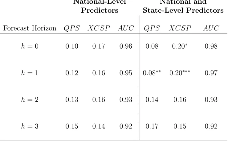
Table 1 presents the forecast evaluation metrics for two alternative models. The first uses

only national-level predictors. This model will serve as our baseline with which to compare

the second model, which includes both national- and state-level predictors. These metrics

tell a consistent story: the model that includes state-level data produces better forecasts than

the baseline model for very short horizon forecasts, namely nowcasts (h = 0) and one-step ahead forecasts (h = 1.) At these horizons, the QP S is lower, while the XCSP and AU C

are higher, for the model including state-level data. For the QP S and XCSP, we further test the null hypothesis of equal forecast accuracy using the Diebold-Mariano-West (DMW)

test, and find that this can be rejected for XCSP when h = 0 and for both metrics when

h= 1.14 _{The forecast improvements as measured by several metrics are quantitatively large.}

As one example, the XCSP is 3 percentage points higher for the model including state-level

data when h = 1, meaning that approximately 12 more months were correctly classified by the model that includes state-level data. For longer horizons, the inclusion of state-level data

appears less helpful. For h= 2 and h= 3, the forecast metrics are very similar for both the

baseline model and the model that includes state-level data.

We next investigate whether the improvements generated by the inclusion of state-level

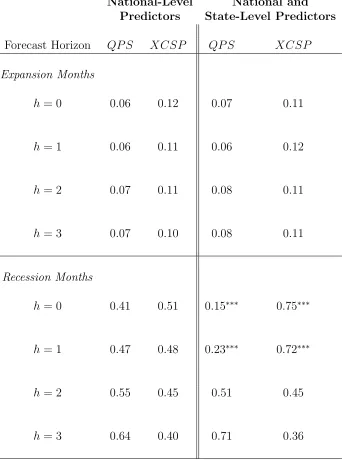
data are symmetric across business cycle phases. Table 2 presents the forecast evaluation

metrics computed separately for expansion vs. recession months in the out-of-sample

pe-riod.15 _{These results demonstrate that the forecast improvements generated by the inclusion}

of state-level data in the out-of-sample period are concentrated in recession months. In

par-ticular, the forecast evaluation metrics computed for expansions are similar for the baseline

model and the model that includes state-level data. However, when we focus on recession

months, there is a clear benefit from incorporating state-level data for short-horizon

fore-casts. For h = 0 and h = 1, the QPS is reduced by 50% to 60% during recession months. The XCSP improvements are approximately 25 percentage points at these horizons, meaning

that a quarter of the recession months over the sample period are correctly classified by the

model that includes state-level data, but not by the model that includes only national-level

data. The QP S and XCSP improvements are highly statistically significant based on the DMW test. There are again no clear improvements from the addition of state-level data at

longer horizons.

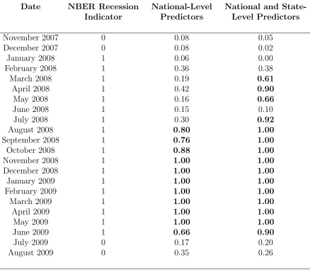
To provide an example from a specific recession, Table 3 presents the out-of-sample

forecasts, Sbt+h, for the h = 1 case around the 2008-2009 recession. Beginning with the

model that includes only national-level variables, Sbt+1 does not cross 50% probability of

recession until August 2008, eight months following the beginning of the NBER-defined

recession. For the h = 1 horizon, this forecast would have been available at the end of July 2008. This is consistent with the considerable uncertainty that persisted well into 2008

about whether the economy had entered a recession phase. For example, the NBER did not

announce the December 2007 peak until December 1, 2008. Also, as discussed in Hamilton

(2011), statistical models designed to track business cycle turning points using national-level

15_{Specifically, the forecast evaluation metrics discussed in Section 2.3 are computed separately for the}

sub-sample of months for whichSt+h= 0 and the subsample of months for whichSt+h= 1. We do not report

data did not send a definitive signal that the recession had begun until mid-to-late 2008.

However, Table 3 also reveals that incorporating state-level data would have provided a

much quicker signal of the beginning of this recession. Specifically, Sbt moved above 50%

probability of recession for March 2008, where this forecast would have been available as of

the end of February 2008, an impressive five month improvement over the model using only

national-level data. Notably, both models produce accurate one-month ahead forecasts of

the end of the 2008-2009 recession.16

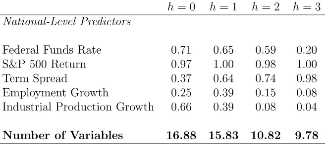
We next evaluate which variables are deemed as important predictors in the BMA

pro-cedure. Table 4 reports the posterior inclusion probabilities for the model that includes

both national- and state-level data, averaged over the recursive estimations conducted to

construct the out-of-sample forecasts. The table provides these inclusion probabilities for all

of the national-level variables. The state-level variables will be discussed separately below.

Of the national-level variables, the S&P 500 return is a robust predictor across all forecast

horizons, with average inclusion probabilities close to 100%. The Federal Funds rate also has

average inclusion probabilities above 50% for several forecast horizons. The term spread

be-comes a more robust predictor as the forecast horizon lengthens, consistent with the finding

of the existing literature that this variable is useful for longer-horizon business cycle phase

predictions. Interestingly, neither aggregate employment or aggregate industrial production

growth have average inclusion probabilities above 50% for most forecast horizons, the single

exception being industrial production growth when h = 0. These variables have very high average inclusion probabilities when state-level data is not included (not reported), implying

the importance of these aggregate level variables is substantially diminished by the inclusion

of state-level data.

The final row of 4 shows the posterior median for the number of variables in the model,

16_{When we extend this analysis to each of the five NBER peaks in the out-of-sample evaluation period, we}

averaged across the recursive estimations. For the h = 0 and h = 1 horizon these values are large, at greater than 15 variables. This suggests that there are a substantial number

of state-level variables that influence the forecast. To investigate which state level variables

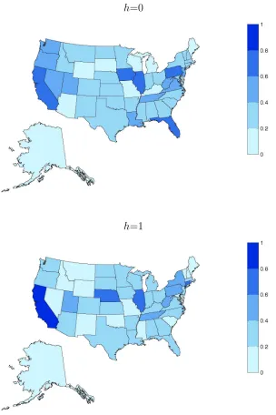
these are, Figure 1 maps the states with ranges of inclusion probability. We focus on the

h = 0 and h = 1 forecast horizons, where the forecast improvements from the addition of state level data are concentrated. These maps show that while there are few states with very

high average inclusion probabilities (darker shading), there are many states with average

inclusion probabilities in the 20%-60% range, meaning a large number of states influence

the BMA forecast. These probabilities also indicate significant model uncertainty regarding

which state-level variables should be included in the model. One likely reason for this

uncertainty is significant correlation between the state-level employment growth variables.

This uncertainty again highlights the potential importance of the BMA approach we take to

select predictors and incorporate uncertainty about this selection.

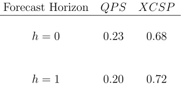
Given this potential importance, we next present results meant to evaluate whether the

BMA predictor selection algorithm is a significant factor for the out-of-sample forecast

im-provements generated with the addition of state-level data. Specifically, Table 5 reports the

forecast evaluation metrics for out-of-sample forecasts produced from a model in which all

national- and state-level variables are always included. As the forecasting improvements from

adding state-level data were concentrated in short-horizon forecasts of recession months, we

focus on the forecast evaluation metrics computed for nowcasts (h= 0) and one-month-ahead forecasts (h= 1) of recession months over the out-of-sample period. By comparing Table 5 to the bottom panel of Table 2, we can gauge the value added of using the BMA predictor

selection algorithm to construct forecasts, vs. simply including all possible variables.

In-deed, this comparison shows a deterioration in the out-of-sample forecast performance from

conditioning on a model that includes all possible variables rather than using BMA. Notably

however, the model with all variables included is still preferred to the model that doesn’t

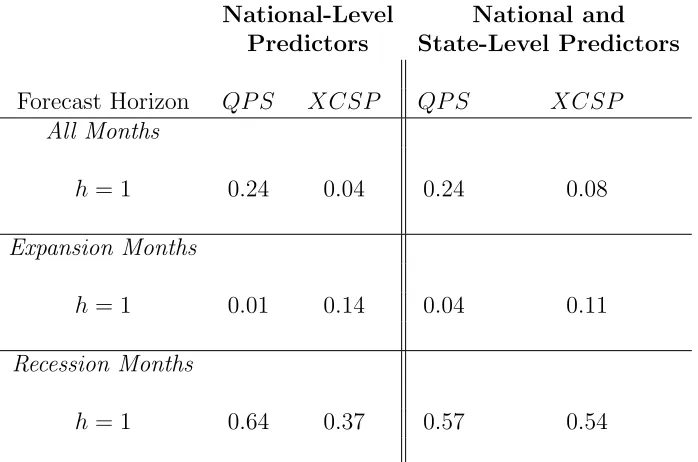
Finally, as was discussed in Section 3 above, our out-of-sample forecasts are constructed

using ex-post revised data for the predictors taken from the September 2013 vintage for each

series. In Table 6 we evaluate the robustness of the out-of-sample forecasting results when

we instead use only vintages of data that would have been available to a forecaster in real

time. Due to difficulties with obtaining long histories for state-level payroll employment at

a substantial number of vintages, we focus on a shorter out-of-sample period running from

July 2007 to June 2011, which includes the most recent NBER-defined recession. As forecast

improvements from the addition of state-level data were primarily at short horizons, we focus

on one month ahead forecasts.

Table 6 demonstrates that our primary conclusions from the longer out-of-sample period

using ex-post data are confirmed for the shorter out-of-sample period using real-time data.

In particular, there is a general improvement in the forecast evaluation metrics computed

for recession months from the addition of state-level data. As an example, the XCSP is 17

percentage points higher when state-level data is included, which corresponds to roughly

3 more recession months during the 2008-2009 recession being correctly classified. Also, as

before, there is no apparent improvement from the addition of state-level data for one-month

ahead predictions of expansion phases.

5

Conclusion

A large literature has investigated the predictive content of variables measured at the

na-tional level, such as aggregate employment and output growth, for forecasting U.S. business

cycle phases (expansions and recessions.) Motivated by recent studies showing differences in

the timing of business cycle phases in nationally aggregated data from those for

geographi-cally disaggregated data, we investigate the information contained in state-level employment

growth for forecasting national business cycle phases. We use as a baseline a probit model

con-sists of national-level economic activity and financial variables. We then add to this model

state-level employment growth. To avoid issues associated with overparameterization of

forecasting models, we use a Bayesian model averaging procedure to construct forecasts.

Using a variety of forecast evaluation metrics, we find that adding state-level employment

growth improves nowcasts and short-horizon forecasts of the NBER business cycle phase over

a model that uses data measured at the national-level only. The gains in forecasting accuracy

are concentrated during months of recession, and are large and statistically significant.

Pos-terior inclusion probabilities indicate substantial uncertainty regarding which states belong

References

Albert, J. H. and S. Chib (1993). Bayesian analysis of binary and polychotomous response

data. Journal of the American Statistical Association 88(422), 669–679.

Berge, T. (2013). Predicting recessions with leading indicators: Model averaging and

selec-tion over the business cycle. Federal Reserve Bank of Kansas City Working Paper No.

13-05.

Berge, T. and O. Jord´a (2011). The classification of economic activity into expansions and

recessions. American Economic Journal: Macroeconomics 3(2), 246–277.

Brier, G. W. (1950). Verification of forecasts expressed in terms of probability. Monthly

Weather Review 75(January), 1–3.

Burns, A. F. and W. C. Mitchell (1946). Measuring business cycles. New York: National

Bureau of Economic Research. ID: 169122.

Carter, C. K. and R. Kohn (1994). On gibbs sampling for state space models.

Biometrika 81(3), 541–553. ID: 476895942.

Casella, G. and E. I. George (1992). Explaining the gibbs sampler. American

Statisti-cian 46(3), 167–174. ID: 481283991.

Chauvet, M. and J. Piger (2008). A comparison of the real-time performance of business

cycle dating methods. Journal of Business and Economic Statistics 26(1), 42–49.

Diebold, F. X. and R. S. Mariano (1995). Comparing predictive accuracy.Journal of Business

and Economic Statistics 13, 253–265.

Diebold, F. X. and G. D. Rudebusch (1991). Forecasting output with the composite leading

Estrella, A. (1997). A new measure of fit for equations with dichotomous dependent variables.

Journal of Business and Economic Statistics 16(2), 198–205.

Estrella, A. and F. S. Mishkin (1998). Predicting u.s. recessions: Financial variables as

leading indicators. The Review of Economics and Statistics 80(1), 45–61.

Gelfand, A. E. and A. F. M. Smith (1990). Sampling-based approaches to calculating

marginal densities. Journal of the American Statistical Association 85(410), 398–409.

Hamilton, J. D. (1989). A new approach to the economic analysis of nonstationary time

series and the business cycle. Econometrica 57(2), 357–384. ID: 480697643.

Hamilton, J. D. (2011). Calling recessions in real time. International Journal of

Forecast-ing 27(4), 1006–1026.

Hamilton, J. D. and M. T. Owyang (2011). The propagation of regional recessions. NBER

working paper no. 16657.

Hand, D. J. and V. Vinciotti (2003). Local versus global models for classification problems:

Fitting models where it matters. The American Statistician 57, 124–131.

Hernandez-Murillo, R. and M. T. Owyang (2006). The information content of regional

employment data for forecasting aggregate conditions. Economic Letters 90(3), 335–339.

Holmes, C. C. and L. Held (2006). Bayesian auxiliary variable models for binary and

multi-nomial regression. Bayesian Analysis 1(1), 145–168.

Katayama, M. (2008). Improving recession probability forecasts in the u.s. economy. Working

Paper.

Kauppi, H. and P. Saikkonen (2008). Predicting u.s. recessions with dynamic binary response

King, T. B., A. T. Levin, and R. Perli (2007). Financial market perceptions of recession

risk. Federal Reserve Board Finance and Economics Discussion Series working paper no.

2007-57.

Mitchell, W. C. (1927). Business Cycles: The Problem and its Setting. New York: National

Bureau of Economic Research.

Owyang, M. T., J. Piger, and H. J. Wall (2005). Business cycle phases in u.s. states. Review

of Economics and Statistics 87(4), 604–616.

Rudebusch, G. D. and J. C. Williams (1991). Forecasting recessions: The puzzle of the

enduring power of the yield curve. Journal of Business and Economic Statistics 27(4),

492–503.

Tanner, M. A. and W. H. Wong (1987). The calculation of posterior distributions by data

augmentation. Journal of the American Statistical Association 82(398), 528–540.

West, K. D. (1996). Asymptotic inference about predictive ability. Econometrica 64, 1067–

1084.

Wright, J. H. (2006). The yield curve and predicting recessions. Federal Reserve Board

Figure 1

Average Predictor Inclusion Probabilities for Recursive Estimations

h=0

h=1

Table 1

Forecast Evaluation Metrics

National-Level National and

Predictors State-Level Predictors

Forecast Horizon QP S XCSP AU C QP S XCSP AU C

h= 0 0.10 0.17 0.96 0.08 0.20⇤ _0.98

h= 1 0.12 0.16 0.95 0.08⇤⇤ _0.20⇤⇤⇤ _0.97

h= 2 0.13 0.16 0.93 0.14 0.16 0.93

h= 3 0.15 0.14 0.92 0.17 0.15 0.92

Table 2

Forecast Evaluation Metrics - Expansion vs. Recession Months

National-Level National and

Predictors State-Level Predictors

Forecast Horizon QP S XCSP QP S XCSP

Expansion Months

h= 0 0.06 0.12 0.07 0.11

h= 1 0.06 0.11 0.06 0.12

h= 2 0.07 0.11 0.08 0.11

h= 3 0.07 0.10 0.08 0.11

Recession Months

h= 0 0.41 0.51 0.15⇤⇤⇤ _0.75⇤⇤⇤

h= 1 0.47 0.48 0.23⇤⇤⇤ _0.72⇤⇤⇤

h= 2 0.55 0.45 0.51 0.45

h= 3 0.64 0.40 0.71 0.36

Table 3

One-Month Ahead Forecasts: 2008-2009 Recession

Date NBER Recession National-Level National and

State-Indicator Predictors Level Predictors

November 2007 0 0.08 0.05

December 2007 0 0.08 0.02

January 2008 1 0.06 0.00

February 2008 1 0.36 0.38

March 2008 1 0.19 0.61

April 2008 1 0.42 0.90

May 2008 1 0.16 0.66

June 2008 1 0.15 0.10

July 2008 1 0.30 0.92

August 2008 1 0.80 1.00

September 2008 1 0.76 1.00

October 2008 1 0.88 1.00

November 2008 1 1.00 1.00

December 2008 1 1.00 1.00

January 2009 1 1.00 1.00

February 2009 1 1.00 1.00

March 2009 1 1.00 1.00

April 2009 1 1.00 1.00

May 2009 1 1.00 1.00

June 2009 1 0.66 0.90

July 2009 0 0.17 0.20

August 2009 0 0.35 0.26

Table 4

Average Predictor Inclusion Probabilities for Recursive Estimations

h= 0 h= 1 h = 2 h= 3

National-Level Predictors

Federal Funds Rate 0.71 0.65 0.59 0.20 S&P 500 Return 0.97 1.00 0.98 1.00

Term Spread 0.37 0.64 0.74 0.98

Employment Growth 0.25 0.39 0.15 0.08 Industrial Production Growth 0.66 0.39 0.08 0.04

Number of Variables 16.88 15.83 10.82 9.78

Table 5

Forecast Evaluation Metrics - Recession Months All National- and State-Level Predictors Included

Forecast Horizon QP S XCSP

h= 0 0.23 0.68

h= 1 0.20 0.72

Table 6

Forecast Evaluation Metrics with “Real-Time” Data

National-Level National and

Predictors State-Level Predictors

Forecast Horizon QP S XCSP QP S XCSP

All Months

h= 1 0.24 0.04 0.24 0.08

Expansion Months

h= 1 0.01 0.14 0.04 0.11

Recession Months

h= 1 0.64 0.37 0.57 0.54