An analysis of non ideal HVDC convertor behaviour in the frequency domain, and a new control proposal

(1)

A

ANALYSIS

ONVERTOR

NON·IDEAL

IN

AND A

CONTROL

ALAN

WOOD

the degree of Doctor

Electronic

lLJALE,'Ulll..., ...

University

Christchurch, New

a....rv ... "L ... JL ....

(2)

(3)

thesis describes a linear and direct method of analysing the interaction of waveform distortion around an HV dc convertor.

Existing analysis techniques are reviewed, and their strengths and weaknesses outlined. Both time domain simulation and iterative harmonic domain solutions are potentially very accurate. However, the lack of insight they provide into the important mechanisms of waveform distortion interaction, coupled with the computational expense (time domain), or limitation to steady state integer harmonics (harmonic domain). are considerable shortcomings. The frequency domain transfer function approach is chosen, and extended to cover the most important mechanisms of frequency transfer.

The developed approach is used first to consider the convertor in isolation, secondly to consider the convertor coupled with either the ac system or the dc system impedance, and finally the convertor embedded within both an ac and dc system. In this way the importance of the different mechanisms of distortion transfer through a convertor are established, the frequency dependent impedance of a convertor is developed, and a description of waveform distortion dynamics around a convertor with realistic ac and dc conditions is achieved. A new indicator, the Saturation Stability Factor, is used to describe the dynamics of transformer core saturation instability.

The linearised frequency domain convertor model is demonstrated to have useful accuracy, and with its ease and speed of use should prove a useful complement to existing analysis techniques.

(4)

(5)

KNOWLE

and foremost, I wish to express my deepest gratitude to my supervisor Professor Jos Arrillaga Without his initial confidence in me, and his continuing support, advice and encouragement, this work: could never have reached fruition.

Many thanks are also due to Dr. Pat Bodger and Professor Hasha Sirisen~ whose involvement during Jos' absence was more valuable to me than I think they realise.

I would also like to express my gratitude to Neville Watson, and the computing staff Mike Shurety and Dave Van Leeuwen for their technical support during the course of my research.

I would also like to thank Transpower NZ (Ltd.) for their financial support.

A special thanks to my postgraduate colleagues, Glenn Anderson, Jose Camacho, Julio DeS-ouza, Dave Gilbert, Stu Macdonald, Dr. S. Sankar, Dr. Mohammed Zavahir, Wade Enright, Maria-Luiza Lisboa, and Dr. Allan Miller for the many discussions and countless distractions they have provided.

These acknowledgements would be incomplete without mention of the many people who were accomplices in escapism. Particular thanks must go to Mike Brewer, Kerry Palmer and Lucette Dijkstra, Catherine Watson, Bruce McCallum, Guy Halliburton, Steve Baker, Sarah McGill, Sarah Gerard and Greg 000.

I would also like to express my appreciation of my partner Margie's love and patience. Without her these years would have been much less fulfilling.

(6)

(7)

ACKNOWLEDGEMENTS _v

1

Chapter 2

Chapter 3

xvii

INTRODUCTION 1

1.1 1.2 1.3 1.4

HV dc systems HV dc-ac interactions Principal objectives Thesis outline

1 2 2 NON· CHARACTERISTIC FREQUENCIES IN HVDC-AC

INTERACTIONS 5

5 5

8

2.1 Introduction 2.2 Historical review 2.3 Analysis techniques

THE TRANSFER FUNCTION 11

3.1 Introduction 11

3.2 The ideal converter transfer function 11

3.2.1 Firing angle modulation 13

3.3 The non-ideal converter transfer function, steady commutation

period 15

3.3.1 The steady state commutation period 15 3.3.2 Converter transfer function to DC voltage 16 3.3.3 Converter transfer function to AC current 17 3.4 The non-ideal converter transfer function, variable commutation

period 19

3.4.1 Commutation period variability 19

Transfer to dc voltage 27

Transfer to ac current 28

Control Transfer functions 30

(8)

viii 4 Chapter 5 Chapter 6 Chapter 7 Chapter 8 CONTENTS

3.5.2 Minimum gamma control 3.6 Conclusions

NON FREQUENCY

4.1 Introduction 4.2 Model verification

4.3 Transfer of WaVefOlTIl distortion 4.3.1 Firing angle distortion 4.3.2 AC voltage distortion 4.3.3 DC current distortion 4.4 Conclusions

CONVERTER 5.1 Introduction

The converter equivalent 5.3 Harmonic impedance

DEPENDENT

5.3.1 Converter impedance viewed from the de side. 5.3.2 Converter impedance viewed from the ac side. 5.4 Conclusions

HARMONIC 6.1 Introduction

AND RESONANCES 6.2 A circuit approach - composite resonance

6.3 A control approach - open loop gain

6.4 The effect of firing angle control on converter impedance 6.5 Case study

6.5.1 A simple control optimisation 6.6 Conclusions

CONVERTER TRANSFORMER '-'...,., ... ,...., SATURATION

30 33 35 35 35 36 37 41 50 59 61 61 63 66 69 72 73 73 74 76 76

79

81

AND RESONANCES 83

7.1 Introduction 83

7.2 Converter tran...:;former core saturation harmonic contribution 83 7.3 Harmonic instability analysis, with no firing angle or

commutation period modulation 85

7.4 Harmonic instability analysis, with firing angle and commutation

period modulation 87

7.5 Saturation stability factor 88

7.6 Case study 89

7.7 Conclusions 94

UNIFIED "-"J:1 ... " ' " TO BACK LINK

(9)

CONTENTS

Chapter 9

REFERENCES

Appendix A

8.2 The traditional control approach 95

8.3 tmified control approach 97

8.3.1 Coordination of firing angles 97

8.3.2 Choice of controlled variables 98

8.3.3 Advantages oftmified control 98

8.4 control system structure 99

8.4.1 angle integral loops 99

8.4.2 Current control 100

8.4.3 Overall gain correction 100

Operating point control 100

8.4.5 Minimum extinction angle control, and firing angle limits 100

8.5 Control system strategies 10 1

8.5.1 Steady state operating point selection 10 1

8.5.2 Dynamic operating point control 101

8.6 Control system strategy evaluation 101

8.6.1 Factors affecting choice of control system strategy. 102 8.6.2 AC/DC system interaction analysis 103 8.6.3 Two alternative ac/dc interaction indicators 106

8.7 Case study 110

8.7.1 Traditional control strategies 110

8.7.2 Alternative control strategies 112

8.8 Conclusions 114

CONCLUSIONS AND FUTURE 9.1 Conclusions

9.2 Future work:

PULSE POSITION MODULATION

117 117

118

THE CONVERTER TRANSFER 129

Al The PPM spectrum 129

A.2 Spectrum of commutation portion of converter transfer functions

that result in de voltage 130

A3 Spectrum of commutation portion of converter transfer functions

that result in ac current 132

A4 Spectrum of commutation period variation portion of converter

transfer functions that result in ac current 133

l11>1I1I1I>11"1OI1II", B PULSE DURATION MODULATION ANALYSIS

THE CONVERTER TRANSFER FUNCTION 137

B.l The PDM spectrum 137

B.2 Spectrum of firing angle modulation applied to the ideal converter

(10)

x

D

FIRING HARMONIC

IMPEDANCE CALCULATIONS D.I Converter de side impedance

D.2 Converter ac side positive sequence impedance D.3 Converter ac side negative sequence impedance

"'l!'M.w",ilIIV E HVDC TEST

E.1 The ClORE model E.2 The back to back model

DERIVATION POWER SENSITIVITY

PUBLISHED PAPER

CONTENTS

141

145

146

(11)

LI

3.1 functions for ideal 6 pulse convertors, phase a 13

3.2 functions for ideal 12 pulse convertor, phase a l3

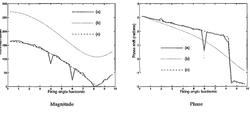
3.3 function for firing angle modulation. . . 14 3.4 Non-ideal transfer function waveform, to dc voltage. 16 3.5 Non-ideal transfer function waveform, to ac current. . 18 3.6 The commutation circuit. . . . 20 3.7 6 pulse convertor thyristor numbering . . . 23 3.8 Commutation period variation transfer function, to ac current. . 29 3.9 Minimum gamma control block diagram. . . 31 3.10 Waveform transfer for 'minimum over previous period' gamma control block. 32 1 Voltage and current conventions around the 12 pulse convertor . . . 36 4.2 CrORE rectifier hannonic transfer, firing angle modulation to dc voltage. 38 4.3 ClORE inverter hannonic transfer, firing angle modulation to dc Voltage. 39 4.4 ClORE rectifier hannonic transfer, firing angle modulation to positive sequence

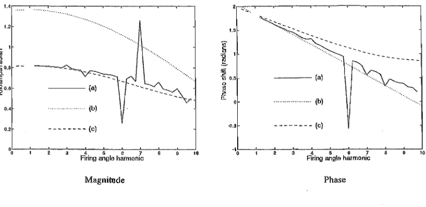
ac current. . . 40 ClORE inverter hannonic transfer, firing angle modulation to positive sequence ac current. . . 42 4.6 ClORE rectifier harmonic transfer, firing angle modulation to negative sequence

ac current. . . 42 4.7 ClORE inverter hannonic transfer, firing angle modulation to negative sequence

ac current. . . 43 4.8 ClORE rectifier hannonic transfer, positive sequence ac voltage to dc voltage.

4.9 ClORE inverter harmonic transfer, positive sequence ac voltage to dc voltage.

4.10 ClORE rectifier hannonic transfer, negative sequence ac voltage to dc voltage. 47 4.11 ClORE inverter hannonic transfer, negative sequence ac voltage to dc voltage. 48 4.12 ClORE rectifier harmonic transfer, positive sequence ac voltage to positive

se-quence ac current. . . 48 l3 ClORE rectifier hannonic transfer, positive sequence ac voltage to negative

se-quence ac current. . . 49 4.14 ClORE rectifier hannonic transfer, negative sequence ac voltage to positive

se-quence ac current. . . . . . 49 4.15 ClORE rectifier hannonic transfer, negative sequence ac voltage to negative

se-quence ac current. . . . . . . . 50 4.16 ClORE inverter harmonic transfer, positive sequence ac voltage to positive

(12)

LIST OF FIGURES

17 inverter harmonic transfer, positive sequence ac voltage to negative se-quence ac current. . . " 51 4.18 inverter harmonic transfer, negative sequence ac voltage to positive

se-4.19 4.20 4.21 4.22 4.23 4.24 4.25 S.l 5.2 5.3 5.4 5.5 5.6 5.7

S.8

5.9 5.10 5.11

quence ac current. . . .

~A''''''''-'-' inverter harmonic transfer, negative sequence ac voltage to negative se-quence ac current. . . . . ClORE rectifier harmonic transfer, dc current to positive sequence ac current. . inverter harmonic transfer, dc current to positive sequence ac current. . rectifier harmonic transfer, dc current to negative sequence ac current. inverter harmonic transfer, dc current to negative sequence ac current.

'_"l'J.L ... 1l.J rectifier harmonic transfer, dc current to dc Voltage.

... , ... inverter harmonic transfer, dc current to dc voltage. System equivalents with convertor. . . . System equivalents with convertor equivalents . . . .

First order non-characteristic frequency interactions around a convertor . ClORE inverter dc side harmonic impedance, without firing angle controL ClORE rectifier dc side harmonic impedance, without firing angle control ClORE inverter dc side harmonic impedance, with firing angle control. . . ClORE rectifier dc side harmonic impedance, with firing angle control . . ClORE inverter ac side harmonic impedance, without firing angle control. ClORE rectifier ac side harmonic impedance, without firing angle control . ClORE inverter ac side harmonic impedance, with firing angle control. ClORE rectifier ac side harmonic impedance, with firing angle control.

51 52 52 54 54 55 59 59 62 62 66 67 68 68 69

70

71 71 6.1 Convertor and dc system electrical and control equivalents . , . . . . 75 6.2 Transfer function for impedance contribution of constant current control 77 6.3 Open loop gain for current control gains, examples 1 and 2. . . . 77 6.4 Closed loop gain for two current control gains, examples 1 and 2. . . 78 6.5 Series impedance of convertor and dc system, examples 1 and 2. . . . . 78 6.6 Rectifier dc current, start-up and response to inverter ac system fault for examples

1 and 2. . . . . 79 6.7 Open loop gain for optimised current control, example 3. . . 80 6.8 Rectifier dc current, start-up and response to inverter ac system fault for optimised

control gain, example 3. . . 80 7.1 Convertor transformer primary magnetising current, with dc offset. 84 7.2 Mechanism of convertor transformer core saturation instability . . 86 7.3 ClORE benchmark rectifier Saturation Stability Factor for current control

magni-tude and phase response. . . 89 7.4 ClORE benchmark rectifier transformer saturation transient response, example 1.. 91 7.5 ClORE benchmark rectifier transformer saturation transient response, example 2.. 92 7.6 ClORE benchmark rectifier transformer saturation transient response, example 3.. 93 8.1 Vd/Id diagram oftypical link: control . . .

8.2 Block diagram of typical HVdc convertor controller. Block diagram of unified controller . . . .

96 97

(13)

LIST OF FIGURES

8.4 Hierarchical levels of HVdc controls with typical time constants (from and IEEE, 1992]) . . . .

8.5 Voltage Stability Factor (VSF) for ClORE benchmark inverter . . . . 8.6 Power curve for ClORE benchmark inverter . . . . 8.7 Convertor terminal voltage vs. remote ac voltage; steady state analysis 8.8 Convertor power vs. remote ac voltage; steady state analysis . . . 8.9 Inverter extinction angle vs. remote ac voltage; steady state analysis .

8.10 Convertor terminal voltage vs remote a.c. voltage; steady state analysis for xiii

104 105 . 106 107 108 108 constant power control . . . 109 8.11 Vd-Id diagram for unified controller . . . 110 8.12 Small inverter disturbance, traditional control . . . III 8.13 Small inverter disturbance, unified control of dc current and inverter extinction

angle. . . . . 111 8.14 Small rectifier disturbance, traditional control . . . 112 8. Small rectifier disturbance, unified control of dc current and inverter extinction

angle. . . . 112 8.16 Inverter short circuit, traditional control . . . 113 8.17 Inverter short circuit, unified control of dc current and inverter extinction angle. . 113 8.18 Dynamic terminal voltage analysis of control strategies for a transient 5% increase

in remote a.c. voltage . . . 114 8.19 Dynamic terminal power analysis of control strategies for a transient 5% increase

in remote a.c. voltage . . . . 114

A.l PPM generation waveforms.

Commutation function waveform for transfer to dc voltage. A.3 Commutation function waveform for transfer to ac current. A.4 Commutation period variation function, for transfer to ac current.

1 generation waveforms. . . . Transfer function for firing angle modulation.

C.l DC voltage harmonic spectrum, algebraically derived C.2 DC voltage harmonic spectrum, simulation derived . C.3 AC current harmonic spectrum, algebraically derived C.4 AC current harmonic spectrum, simulation derived . E.l Single line diagram of ClORE benchmark HV dc test system E.2 ClORE inverter ac system frequency dependent impedance E.3 ClORE rectifier ac system frequency dependent impedance E.4 ClORE dc system frequency dependent impedance . E.5 Single line diagram of back to back HVde test system . . . FJ System and vectors for steady state analysis of sensitivity factors.

(14)

(15)

LIST OF TABLE

3.1 Firing angle modulation transfer function multipliers (b=3 degrees or 0.0524 radians) 15 3.2 Distortion of commutation voltages. . . 24

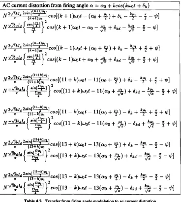
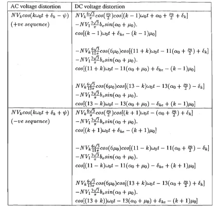
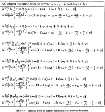
4.1 Transfer from firing angle modulation to dc voltage distortion . 4.2 Transfer from firing angle modulation to ac current distortion 4.3 Transfer of ac voltage distortion to dc voltage distortion . . 4.4 Transfer from dc current distortion to ac current distortion. 4.5 Transfer from dc current distortion to dc voltage distortion

6.1 Current control gains for test case examples. . . .

7.1 Saturation stability factor for test case examples.

8.1 Voltage Sensitivity and Power Sensitivity for different control types, steady state 38 41 46 53 58 79

90

analysis . . . 108 8.2 Voltage Sensitivity and Power Sensitivity for different control types, from dynamic

simulation . . . 115

E.l Reactive compensation and Transformer ratios for different steady state operating

points . . . 151

(16)

(17)

b

jam J

ms

N

s

Vcom

Firing angle modulation magnitude End of commutation period magnitude

Duration of commutation period modulation magnitude (see definition in section 3.4.1.4)

Modulation of firing angle Bessel function of the first kind

Modulation of end of commutation period

Modulation of duration of effective commutation period (see definition in section 3.4.1.4)

Average value of convertor dc side current Instantaneous value of convertor dc side current

Instantaneous phase current on ac system side of convertor transformers Equivalent inductance of convertor transformer leakage, referred to

convertor side of the transformer

Equivalent inductance of convertor transformer magnetisation, referred to convertor side of the transformer

Milliseconds

Convertor transformer ratio, convertor side to ac system side Seconds

Time

Average value of convertor dc side voltage Instantaneous value of convertor dc side voltage

Instantaneous phase voltage on ac system side of convertor transformers Fundamental phase voltage peak magnitude on ac system side of

convertor transformers

Fundamental phase voltage rms magnitude on ac system side of convertor voltage magnitude of frequency kwo on ac system side of convertor transformers

(18)

Wo

side of convertor transformer

Fundamental frequency peak commutation voltage on convertor side of convertor transformer

GLOSSARY

Convertor transformer fundamental frequency leakage reactance, referred to convertor side of the transformer

Convertor transfer function for phases a, b, and c. Instantaneous value of convertor angle order Average value of convertor firing angle order

1f minus convertor extinction angle Convertor extinction angle

Phase angle of distortion frequency

kwo

relative to the phase a fundamental frequency component

0, 120 and 240 degrees, referring to phases a, b and c Actual convertor commutation period duration angle Average convertor commutation period duration angle Effective convertor commutation period duration angle

(see definition in section 3.4.1.4) AC side fundamental frequency

The following valiables are considered as a set. based around a dc side frequency

kwo.

a positive sequence ac side frequency of

(k

+

1

)wo,

and a negative sequence ac side frequency of

(k - 1

)wo.

They are written as vectors with a magnitude and a phase, and refer to either the dc terminals of the convertor or the ac system terminals of the convertor transformer.

Yo

Zdch

Zacp

Zacn

Zxp

Zxn

Zacpx

Zacnx

DC system current at

kwo

AC system +ve sequence current at

(k

(19)

GLOSSARY

Zconvacp

Zconvacn

Zconvdch

()

ESCR HVde MAP PDM PI SCR SSP VSF

Convertor ac side +ve sequence impedance at (k

+

1 )wo

Convertor ac side -ve sequence impedance at (k - 1 )wo

Convertor dc side impedance at kwo

Characteristic angle of impedance Z with the same subscript

Conference Intemationale de Reseaux Electriques Electromagnetic transient de program

Effective Short Circuit Ratio High Voltage direct current Maximum Available Power Pulse Duration Modulation Proportional/Integral Pulse Position Modulation Short Circuit Ratio

(20)

(21)

Chapter 1 INTRO

N

The success of HV dc technology applied to the interconnection of ac systems has been confinned by the rapid growth in its utilisation. There are at present some 50 dc links around the world, with a transmission capacity of about 36000 MW. [Elahl et

at.,

1993]. Although most of these involve transmission by overhead line and/or cable, a significant number are single point back-to-back links. A high level of reliability, coupled with the advantages of very fast controllability, low transmission losses, suitability for cable transmission, and asynchronous connection, all combine to ensure the future of HVdc in modem power systems.

ac'·ac interactions

As convertor ratings have increased, their effect on overall power system dynamics has grown. These HVdc-ac interactions can be divided into three broad categories, related to frequency, voltage, and distortion regulation, briefly summarised below.

AC system frequency is tied to generator rotor speeds, which is in tum related to the balance of generated and absorbed real power in the ac system. The fast controllability of HV dc power allows ac system frequency to be quickly stabilised following a transient. Most modem HVdc installations have some form of power modulation related to ac system frequency, and this is one of the most common ways in which ac system operation is enhanced by HV dc control.

AC system fundamental frequency voltage levels are related to the absorption and generation of reactive power in the network. Reactive power is also quickly controllable at HV dc convertor terminals, although usually at some extra cost. While a rectifier generally enhances the ac system voltage regulation, this is not the case at an inverter, where controllable reactive compensation or novel convertor control schemes may be required. The best approach to this sort of interaction is different from installation to installation, and constitutes a continuing challenge to HV dc research and design engineers.

The interaction of current and voltage distortion around an HV dc convertor is related to system and convertor non-linearites and frequency dependent impedances, and is the least well understood of HVdc-ac interactions. Although these interactions can be quite accurately modelled by numerical methods, often problems involving waveform distortion are solved during HVdc commissioning and testing.

(22)

2 CHAPTERl INTRODUCTION modelling teclmiques, coupled with the growing accessibility of digital computing power, has led to numerical analyses of HYdc systems playing a pivotal role in their design and assessment.

1.3 Principal objectives

Most of the research effort described by this thesis was motivated by the desire to improve understanding of the interactions between HYdc convertors and ac and dc systems. The most complex of these interactions are .those involving waveform distortion, and a primary goal was to model these as simply and accurately as possible.

Waveform distortion around a convertor is usually studied using numerical teclmiques with fast digital computers, or analogue hardware simulators. Insights can only be gained by making many analyses with different system parameters, and observing the effects of each change. A linearised non-numerical convertor model has the advantage of offering a direct insight into the important mechanisms of convertor operation, and to develop such a model was the first objective. One of the reasons to develop such a model was to clarify the importance or otherwise of different mechanisms in the HYdc conversion process, which in tum may allow optimisation of HYdc convertor control from the point of view of waveform distortion.

The response of a piece of equipment to a frequency, at that frequency, is important for the overall system dynamics, and at present is only obtainable for the HYdc convertor via time consuming numerical teclmiques. Once the validity of the linear model was established, the next goal was to use it to directly determine the convertor frequency domain equivalent impedance.

The final aim was to apply the model to two common situations in HYdc convertor operation that involve wavefonn distortion, and develop criteria to measure waveform stability. The first situation was a simple transient recovery, and the second, transient recovery involving convertor transfonner core saturation.

An early objective that led to this work was the development and evaluation of a unified control system for a back to back HYdc link:. This work is also reported.

Thesis outline

Chapter 2 introduces the subject of non-characteristic frequency interactions between convertors and dc and ac systems, with a brief literature review and a survey of analysis teclmiques.

A linearised frequency domain convertor model is developed in chapter 3. Three levels of complexity are presented, being for the ideal convertor, the non-ideal convertor with a steady commutation period, and the non-ideal convertor with a varying commutation period.

The model is used to predict harmonic transfers across a convertor in chapter 4, and the low order predictions are checked by dynamic simulation. The relative importance of some features of the convertor model are discussed.

In chapter 5 the concept of a convertor frequency domain equivalent is introduced. By simplifying the convertor model and including either the ac or dc system equivalent impedances, tenns are developed to describe the harmonic impedance of an HVdc convertor from both the dc and ac sides.

(23)

1.4 THESIS OUTLINE 3 Continuing with this theme, chapter 7 introduces the effect of convertor transformer core saturation to the overall system. The damping of this form of distortion is predicted, and checked by dynamic simulation. The Saturation Stability Factor is developed, providing a measure of this sort of system interaction.

With a slightly different emphasis, chapter 8 presents the development and evaluation of a unified control for a back-to-back HVdc link control system.

(24)

(25)

RACTERI

INTERACTION

Introduction

Non-fundamental frequencies are of major importance around an HVdc link. They can be considered as a fonn of power system pollution, where not only can they interfere with con-sumer equipment, but can also interfere with the HVdc commutation process [Kristmundsson and Carroll, 1990], affect protection relay operation, cause overheating of filters or machines, increase dielectric stresses and interfere with communication circuits [Arrillaga et al., 1985].

Non-fundamental frequencies include the characteristic convertor harmonics, non-characteristic harmonics, and non-integer multiples of fundamental frequency, and can occur both in the steady state and transiently.

The characteristic harmonics associated with a dc convertor are well known [Arrillaga

et al., 1985], and usually effectively controlled by suitable filtering orincreasing the pulse number

of the convertor. These harmonics are always present, and are in general a steady state problem. Control of characteristic harmonics is not addressed here.

Steady state non-characteristic harmonics arise from a number of causes, typically a system imbalance, fundamental frequency pick-up on the dc line, or non-linearities in the ac system. These most commonly occur at integer harmonics.

Transient non-characteristic frequencies exist as a result of any system deviation from the steady state, and are not confined to integer harmonics. Observation of many transient waveforms reveals that one or more lightly damped non-characteristic frequencies often dominate a system transient response. This type of wavefonn distortion is related to the ac system, the convertor, and the dc system characteristics. For an understanding the full dynamic interrelationships must be defined.

There are two distinct problems to be considered. Firstly, the steady state frequency spectrum must be defined, and secondly the damping of any transiently occurring distortion should be examined. In either case the interactions between the non-characteristic frequencies around the HVdc convertor need to analysed.

The remainder of this chapter gives an historical review of the analysis of non-characteristic harmonic interactions with HVdc convertors. The techniques themselves are briefty summarised, and a need for a non-numerical frequency domain approach to be extended is identified.

2.2

Problems with non-characteristic harmonics were reported by a number of authors [Last et al., 1966J,

(26)

6 CHAPTER 2 NON·CHARACTERISTIC FREQUENCIES IN HVDC·AC INTERACTIONS first analysis of non-characteristic harmonic interactions with an HVdc convertor came when [Ainsworth, 1967] identified a mechanism of harmonic instability related to individual firing an-gle control. Using an analytical approach based on harmonic symmetrical component theory, but assuming no commutation period and steady dc, he showed how the convertor could return harmonic currents in such a way as to amplify that harmonic. He proposed the phase locked oscillator control system as a solution [Ainsworth, 1968], which has since been widely adopted.

The phenomenon was subsequently examined numeIically [Reeve and Krishnayya, 1968], [Reeve et al., 1969], and algebraically [Phadke and Harlow, 1968], all of whom assumed no

harmonic current on the dc side of the convertor.

[persson, 1970] proposed a set of conversion factors for distortion around a grid controlled convertor. He approximated the effect of the commutation period and allowed for harmonics to present on the dc current. The control systems could be accounted for, both the rectifier and the inverter with their ac systems were modelled, and ultimately a Nyquist plot was generated to analyse system stability. The calculations, however, were sufficiently laborious to require the use of a digital computer. This paper, although ahead of its time in modelling so many interactions, did not clearly establish the relative importance or modelling accuracy of each. Unjustifiably it has been largely ignored in the academic press.

[Reeve and Baron, 1970] took an iterative approach to consider the harmonic voltage developed on the dc side of the convertor. They generalised the approach [Reeve and Baron, 1971] to allow for the ac side current and voltage interaction, but without considering the dc line currents that may result. This, however, was an early step in establishing the likely importance of dc side harmonics.

[Sucena Paiva and FreIis, 1974] viewed the HVdc convertor as a modulator, and generated sinusoidal carrier functions to model the transfer of waveform distortion through the convertor. Like Persson, they considered a complete dc link connecting weak ac systems, included the effect of the control systems, and took the describing function approach of considering only the disturbing frequency. They also utilised the functions to Nyquist plots, and although their approach was simpler than Perssons, useful accuracy was maintained. It was also shown that self-sustained oscillations need not be synchronised with the ac system frequency.

[Mathur and Sharaf, 1977] took a frequency domain approach to the generation of dc side voltage and current harmonics as a result of ac side voltage distortion, or control/ac system imbalances. The commutation process was considered, but the consequential effects of dc side harmonic current was not considered. The analysis used numerical frequency domain techniques to obtain the harmonic interrelationships.

[Ainsworth, 1977] reported on an instability related to convertor transformer core saturation in the Kingsnorth scheme, where a firing angle modulation scheme was provided as a solution. This was the first example of control of harmonic problems by active modulation of the convertor firing angle.

[Yacamini and de Oliveira, 1980b] demonstrated that the form of harmonic instability provoked by convertor transformer core saturation can only be shown if finite ac and dc side impedances are used. They performed an analysis based on an iterative technique reported in an earlier paper [Yacamini and de Oliveira.. 1980a], and proposed that an instability was indicated when the iterative procedure failed to converge. Based on

ac/dc

side interaction, they suggested the possibility of an instability is independent of the control system and transformer saturation. The importance of dc side harmonic currents was established beyond doubt.

The need for a better understanding of dc system resonances was addressed by [Bahrman

(27)

2.2 HISTORICAL REVIEW 7 attempted to quantify its effect. They also noted the significance of the convertor current control, and described an apparent resistance in the convertor dc side impedance due to commutation period variation.

[Yacamini and de Oliveira, 1986] offered a comprehen..'live iterative approach to finding har-monics in large convertor systems, considering the commutation process, controls, and ac and dc side harmonic currents.

[Stemmler, 1987] used steady state convertor transfer functions in an algebraic analysis of a convertor core saturation instability on the Blackwater back to back intertie. Neglecting com-mutation and firing angle control, but considering the relevant ac and dc side harmonic currents, he proposed a simple instability criteria, and reported on a form of firing angle modulation that damped the instability. This paper demonstr.ated the value of applying a simplified theoretical analysis, and the viability of firing angle control to damp the phenomena.

In the same year, [Ferreira et al., 1987] applied a describing function analysis to HVdc system harmonic stability. Modelling the convertor in a similar way to that of [Yacamini and de Oliveira, 1980b], they iteratively derived the convertor describing functions, and predicted the possibility of harmonic limit cycles for an unbalanced ac system voltage or small second harmonic positive sequence distortion.

[Shore et al., 1989] proposed a new model for the analysis of dc side harmonics in HVdc systems, called the three pulse model. Developed to include the effect of stray capacitances in the convertor station, it correctly predicts dc side triplen harmonics, and revises the magnitude of the ground mode characteristic harmonics. This analysis has particular relevance to dc filter design and telephone intetference problems.

The practicality of controlling harmonic instabilities by special firing angle control was demon-strated in [Bodger et al., 1990], and again in [Kaul and Mathur, 1990]. [Farret and Freris, 1990] reported on an analysis describing the effect of modulating a convertor firing angle, and proposed the possibility of cancelling steady state harmonics by this method.

Convertor transfer functions were used again [Rashid and Maswood, 1988] to analyse harmonic generation in a convertor due to unbalanced ac voltages, which was improVed on by [Sakui and Fujita, 1992]. Both these analyses neglected the effect of any firing angle variation.

A transfer function derived from the Fourier transform of the ac current waveform was used by [Hatziadoniu and Galanos, 1988]. Combined with the ac system characteristics, they predicted the uncontrolled response of an inverter/ac system to a step change in dc current. The model used was quite simple, and didn't allow for convertor control or dc system characteristics, but gave good agreement with the simulated results. This was a promising demonstration of the use of the frequency domain to determine transient response characteristics.

[Larson et al., 1989] used numerical methods.to determine linear relationships between har-monics on either side of a convertor. Using a matrix formulation, and considering ac side harmonic impedance, dc side harmonic. impedance, and the convertor control system, they arrived at terms for the overall harmonic impedance at both the convertor ac and dc terminals. This describing function style of analysis accounted for the harmonic interactions with minimal computation, once the linear relationships had been obtained. The paper used the harmonic impedance of a convertor as a tool to predict lightly or even negatively damped harmonics. As in Stemmler's and Hatziadoniu's papers, a steady stale analysis was used to predict system dynamics.

In the accompanying discussion, Anderson reported using a similar matrix formulation based on the transfer functions developed by Persson in 1970.

(28)

CHAPTER 2 NON-CHARACTERISTIC FREQUENCIES IN HVDC-AC INTERACTIONS

improved on the commutation modelling, and extended the analysis to a 12 pulse convertor and to include the effects of harmonic transfer from the remote end convertor. In their analysis however, the effect of the firing angle variation was neglected.

[Reeve and Subba Rao, 1973] were the first to use time domain simulation as a hannonic analysis tool. Since then, as the development of time domain analysis tools has advanced, a number of authors have used the time domain in harmonic analyses [Kitchin, 1981] [Bodger et al., 1990],[Kaul and Mathur, 1990]. These let a test case be simulated to a good level of accuracy, allowing dynamic variation of waveform distortion levels to be observed.

Analysis

techniques

Although the sophistication of harmonic analysis techniques applicable to HVdc convertors has grown, the methods of analysis can still be split into three broad categories.

Firstly there is the direct frequency domain approach. Linear relationships are assumed be-tween non-characteristic frequencies around the convertor, allowing a relatively fast solution of the convertor in.teractions with its surrounding network. These relationships can be obtained to varying levels of accuracy by algebraically derived transfer functions, or numerical Fourier transforms of observed time domain waveforms. [persson, 1970] developed an algebraic de-scription of the relationships, as did [Sucena Paiva and Freris, 1974] to a certain extent, while [Larson et al., 1989] and [Ferreira et al., 1987] derived them by numerical methods. A num-ber of authors have either used or presented partial descriptions of harmonic interactions, by direct [Ainsworth, 1967], [phadke and Harlow, 1968], [Stemmler, 1987], [Rashid and Mas-wood, 1988], [Sakui et al., 1989], [Farret and Freris, 1990], [Sakui and Fujita, 1992],and [Hu and Yacamini, 1992], or numerical [Hatziadoniu and Galanos, 1988] techniques. To date, how-ever, these techniques do not seem to have become very popular. A special case is the three pulse convertor model [Shore et ai" 1989], which directly and simply models some otherwise

inexplicable dc side harmonics.

Secondly, there is the iterative frequency domain approach, which models the convertor operation more accurately using the convertor equations, and may allow for any number of interconnected items of ecluipment. A harmonic instability might or might not be indicated by failure of the iterative technique to converge. In general these techniques work in the frequency domain for the ac and dc systems, and in the time domain for the convertor itself. The numerical Fast Fourier Transform and its inverse are used to interface between the two domains,

This approach has been developed and used to an increasing level of complexity by [Reeve and Krishnayya, 1968], [Reeve et al., 1969], [Reeve and Baron, 1970], [Reeve and Baron, 1971], [Mathur and Sharaf, 1977], [Yacamioi and de Oliveira, 1980a], [Yacamini and de Oliveira, 1980b], [Ya-camini and de Oliveira, 1986], [ArriUaga et al., 1987] and [Arrillaga and Callaghan, 1991]. Ultimately the approach provides a steady state solution only, and little information is revealed about lightly damped harmonics which may delay recovery from transients.

(29)

2.3 ANALYSIS TECHNIQUES

Due to the complexity of the interactions and the ready availability of digital computers, numerical approaches to harmonic analysis have been rather more popular. However, the direct frequency domain approach, particularly one based on direct descriptions of harmonic interrela-tionships, is the most likely to provide insights into the mechanism of harmonic interactions, and thus into methods of controlling them.

Frequency and time domain numerical methods describe the harmonic interactions for a given example, and as such provide a suitable means for testing different convertor control strategies or circuit configurations. However, the direct relationships that a non-numerical frequency domain approach may provide, offer the' best chance of understanding the harmonic interactions around a convertor, and should lead to the most well informed choice of filters or control strategies.

(30)

(31)

Chapter 3 THE CO V RTOR TRAN FER FUNCTION

Introduction

fu this chapter direct algebraic relationships between distortion on the ac side, the dc side, and in the control of an HVDe convertor are developed. Although the convertor is a non-linear device,

it can be described as a modulator that has approximately linear characteristics in the frequency domain. The analysis is based on a frequency domain description of the conduction and non-conduction periods of the convertor thyristors, which can then be used to describe the interactions around the convertor. In many cases the relationships are non-linear, but limiting distortion to low levels allows linear approximations. This limitation also ensures that the sequence of thyristor conduction periods remains unaffected. The initial analysis is made for a six pulse convertor, and equidistant firing is assumed as the convertor control basis.

Section 3.2 outlines the principle behind the frequency domain based convertor transfer function, and states the functions for an ideal convertor with no commutation period. Section 3.3 introduces the effect of a constant duration commutation period. Section 3.4 describes the variation of the commutation period duration, and incorporates its effect.

The transfer function is gradually built up by summing the described effects. The final function forms the basis of the analyses in chapters 4,5, 6 and 7.

3.2 The ideal convertor transfer function

The transfer function for a convertor describes the conduction and non-conduction periods of the thyristors, referred through the transformer connections. The simplest transfer function assumes ideal convertor transformers which leads to no thyristor conduction overlap, and this is the function used in this analysis. The ideal transfer function has been applied to harmonic studies by [Stemmler, 1987] for a convertor with a steady firing angle. How to consider the thyristor conduction overlap, or commutation period, is discussed in section 3.3.

Before the analysis can proceed, the type of distortion being transferred needs to be examined. As the analysis is undertaken in the frequency domain, the distortion is specified accordingly. Any steady state distortion can be described as the sum of a set of frequencies with appropriate phase and magnitude. Each frequency source is considered singly, the final result being the superposition of the individual results.

Firstly, the three phase ac voltage is described, with a single superimposed frequency. For a positive sequence frequency

(32)

12 CHAPTER 3 THE CONVERTOR TRANSFER FUNCTION while for a negative sequence frequency

(3.2) and for a zero sequence frequency

(3.3) where k is the harmonic order and ~) is 0, 120, and 240 degrees respectively.

The dc cunent and conveltor firing angle can be written as follows

(3.4 ) and

(3.5)

In this way all the fmTIls of distortion are described with a phase reference to the rising zero crossing of the fundamental component of the phase a commutating bus voltage.

The 6 pulse ideal convertor transfer function for a star-star connected transformer with a stead y convertor firing angle, related to each phase of the described voltage waveform and written as a Fourier series is

2V3

1

Y",

= -

I)±)-cos[m(wot -

ao -1/J)]

1[' m

(3.6) m

where

(±) = sin(

~1[')

(3.7)

for m = 1,5,7, 11, etc.

This series has values of 1, 0 or -1, and describes the interconnection between the ac and dc sides of the convertor. 1 signifies a connection of the dc side positive bus to the phase in question, -1 signifies a connection of the dc side negative bus to the phase in question, and 0 indicates no connection.

A similar transfer function can be written for the ideal star-delta connected 6 pulse convertor.

2V3

1

Y", = -

L:(=f)-cos[m(wot -

ao -1/J)]

1[' m m (3.8)

where

(=f)

=

~sin(~1[')

(3.9)

for m = 1,5,7, 11, etc.

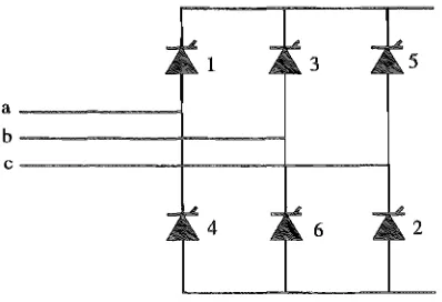
The transfer functions are drawn for a steady firing angle a = 0 in figure 3.1(a) and (b).

In a 12 pulse arrangement, the two 6 pulse convertors are connected in parallel on the ac side and in series on the dc side. H the transfer function is restricted to transfenal of ac voltage to dc

voltage, and dc current to ac current, the two functions can be summed to give the ideal 12 pulse transfer function.

4V3

1

Y",

= -

L:(±)-cos[m(wot -

ao -1/J)]

1[' m m

(3.10) for m == 1, 11, 13,23, etc.

Y1jJ describes the conduction pattern of the thyristors in the 12 pulse convertor, and is illustrated

(33)

3.2 THE IDEAL CONVERroR TRANSFER FUNCTION Ya .... -~---, I I I I Va 13

2 Ya

j3 1---1 _, _,

, ,

1 : Va 1

j3 ---.

---1

e

, ,

L

_________ :

1

-1

I I I

I I

_ _ _ _ _ _ _ _ _ J

-1

j3 ~ j _________ J

I :

t _________ J

- 2

j3

(a) Star-star connection (b) Star-de1ta connection

Figure 3.1 Transfer functions for ideal 6 pulse convertors, phase a

1+..L j3 1+_1_ j3 1 j3 -1 J3 _1 __ 1_

j3 -1- ..L j3 Va r---, , , , , , ,

) ____ J L ____

1

I

t ____ _

I I I I I

l ____ _

I I I

I I

L _________ I

Figure 3.2 Transfer functions for ideal 12 pulse convertor, phase a

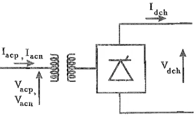
The convertor dc side voltage comprises the sum of the contributions of all three phases

(3.11)

and the convertor ac side current has three values

i.p

=

NY.pid (3.12)

where N is the convertor transformer ratio, secondary/primary .

.

,

3.2.1 Firing angle modulation

In a controlled convertor, each step in the transfer function is delayed by the firing angle a as described by equation 3.5. The variability of the firing angle has to be incorporated into the transfer functions if they are to be of practical use.

(34)

CHAYfER 3 THE CONVERTOR TRANSFER FUNCTION

Va

~,---r, I

: Va

I

(a)

I

I I I

fw 8

-1 .1..--. _ _ _ - - - ' - - '

-

-(b) flu flu

flu flu

-1

Figure 3.3 Transfer function for firing angle modulation.

The dashed line of figure 3.3(a) represents the ideal transfer function, and the solid line the same function modified by a firing angle modulation of L).a. The difference between these two

functions is represented by 3.3(b), called the Jam transfer function. The Jam transfer function can be described as the sum of four pulse trains, one each for the leading and trailing edges of the positive and negative going parts of the ideal transfer function. Adding these pulse trains to the unmodulated transfer function result in the modulated transfer function. The pulses in each train occur once every fundamental cycle, and each pulse starts at the same relative angle and is of a duration proportional to the firing angle deviation from its average value at the instant of firing. A pulse duration modulation analysis based on the spectrum developed by [Schwarz et al., 1966]

is made in appendix B for a six pulse star connected convertor. The resulting spectrum is

V3

~ Jo(mb) - 1

Y.p(t) = -

L./±)

cos[m(wot - ao - 'IjJ)]

1l' m m

2V3

00 I_{n (}mb) 1l'

+ -

L L(±)

cos[(m

+

nk)wot - mao

+

n(ok -

-2) -

m'IjJ] 1l' m n=l m

2V3

00 I_{n (}mb) 1l'

+ -

L L(±)

cos[(m - nk)wot - mao - n(ok

+ -) -

m'IjJ] (3.13)

1l' m n=l m 2

for m = 1,5,7, etc., for a firing angle modulation as specified in equation 3.5, and where J is a

Bessel function of the first kind.

Adding this to the unmodulated spectrum, results in the overall spectrum

V3

Jo(mb)

+

1

Y.p(t)

= -

L(±)

cos[m(wot - ao - 'IjJ)]

1l' m m

2V3

00 I_{n (}mb) 1l'

+ -

L L(±)

cos[(m

+

nk)wot - mao

+

n(ok -

-2) -

m'IjJ] 1l' m n=l m

+

2V3

L

I)±)

In(mb) cos[(m - nk)wot - mao - n(ok

+

~)

-

m'IjJ] (3.14)

(35)

3.3 THE NON-IDEAL CONVERTOR TRANSFER FUNCTION. STEADY COMMUTATION PERIOD 15 for m 1, 5,7, etc.

Extending this to a 12 pulse convertor is simply a matter of doubling the magnitude of the expression and taking only the terms for m = 1, 11, 13, etc.

Table 3.1 gives an indication of the relative amplitudes of some of the terms in the expression, for a firing angle modulation of b

=

3 degrees.

m

1 .9993 .0262 .0003 .0000 .0000 11 .0835 .0251 .0037 .0004 .0000

13 .0683 .0247 .0043 .0005 .0000 23 .0291 .0217 .0070 .0014 .0002

25 .0246 .0210 .0074 .0017 .0003

Table 3.1 Firing angle modulation transfer function multipliers (b=3 degrees or 0.0524 radians)

From table 3.1 it is apparent that the most significant terms of the series are those associated with the Jo~b) and Jl ~b) multipliers. In particular, Jl~b) only decreases very slowly with increasing m. Therefore the terms of frequency (m

±

k

)wo

and

mwo

are of the most significance. Both these terms are non-linear with modulation amplitude, slowly decreasing as the modulation amplitude increases.

A feature of this spectrum is the proliferation of frequencies, many of which will be of significant magnitude. This implies that firing angle control, while possibly able to control the levels of a single steady state unwanted frequency, may not be very effective at reducing overall distortion levels.

3.3 The non-ideal ...

nl'1tll'l/J'II"'t .... r 11'."6]>11"'1,"'11'",,11'"

function, steady C01IDIl[)U1tatllon

period

The first improvement to be made to the ideal transfer function is to include the effect of a steady commutation period. This requires the transfer function to be separated into two distinct functions, one for the transfer of ac voltage to the de side, and one for the transfer of de current to the ac side. Transfer of ac voltage to the de side is exactly modelled by averaging the two commutating voltages during the commutation period. and the current transfer from one phase to the next during the commutation period is linearly approximated. Firstly the commutation period is defined, and then it is incorporated into the transfer functions.

3.3.1 commutation period

The steady state commutation period is easily calculated from the convertor steady state equations. [Arrillaga, 1983], its example of a commutation analysis, develops the equation

Id =

~Yc

(cosao - cos(ao

+

JLo)]

v

2Xc

(3.15)

for a steady dc current and where

Yc

is the phase to phase rms ac voltage at the convertor transformer primary. This is easily revised to

(36)

16

CHAPTER 3 THE CONVERTOR TRANSFER FUNCTION

where Vl is the peak single pha..<;e ac voltage at the convertor transformer primary and Xc is the convertor transformer leakage reactance referred to the convertor transformer secondary.

The steady state commutation period affects the convertor transfer functions differently, de-pending on whether the transfer is to dc voltage distortion or ac current distortion. Both these cases are dealt with separately in the following subsections.

3.3.2 Convertor transfer

." .. ""''ll1'OR

to

voltage

The models used by [Hu and Yacamini, 1992], [Sakui and Fujita, 1992], and [Sakui et al., 1989] for a 6 pulse convertor with a steady firing angle, provide a good basis for considering convertor voltages. Based on the standard commutation process analysis, [Arrillaga, 1983], they modelled the transfer of vol tage from the ac side to the de side of the convertor during the commutation period by averaging the two commutating phase voltages. This changes the shape of the unmodulated transfer function for a 6 pulse convertor as depicted in figure 3.4.

Ya

(a)

-1

0.5

(b)

-0.5

Figure 3.4 Non-ideal transfer function wavefonn, to dc voltage

The dashed line in figure 3.4(a) represents the unmodulated ideal transfer function, and the solid line the function revised to include the commutation process. Figure 3.4(b) represents the difference between these, and is called the commutation function. When firing angle modulation is applied, the pulses of the commutation function are position modulated accordingly. The analysis of the spectrum of the commutation function, based on Schwarz's Pulse Position Modulation (PPM) spectrum [Schwarz et al., 1966] is undertaken in appendix A. Remembering that the position of each rectangular pulse is directly affected by the convertor firing angle, the commutation function is considered as the sum of four position modulated rectangular pulse trains. The spectrum of the commutation function, with firing angle modulation as described by equation is

Y1/J(t)

2v'3 '\:""'"

11" L-t(±)sm(-2-)

.

mJl.O Jo( m mb ) cos[mwot - m(ao

+

2") -Jl.O 2 11"

+v'3

11"

v'3

+

m

11" m

00 (±) In(mb) cos[(m _ nk)wot _ m(ao

+

po) - n(lik

n=l m

m"p]

~) 2

11"

(37)

3.3 THE NON-IDEAL CONVERTOR TRANSFER FUNCTION, STEADY COMMUTATION PERIOD

17 f(±)

In(mb) cos[(m

11" m n=l m

nk)wot mao (3.17)

for m

=

1,5,7, 11 etc. Adding this to the similarly modulated ideal transfer function spectrum (from equation 3.14) yields

Y,p(t) -L,;(±) 2J3 ' " Jo( mb)

+

1

+

2Jo( mb )sin(

11" m 2m

cos[m(wot - ao - 'l,b)]

+

V3

L

fC±)

JnCmb) cos[(m + nk)wot - m(ao + flO)

+

n(lik - kf.LO -

~)

- m'l,b]

11" m n=l m 2

+

V3 '"

_11" _~_~

~(±)J,IlJmb)cos[(m

_m _nk)wat _{m(ao +}_{flo) - n}( 1 1 "

15k - kf.LO

+

2")

m'l,b]

+

V;

~

E(±) JnC:b) cos[(m + nk)wot - maO + n(t5k -

~)

- m'l,b]

+

V;

~E(±)Jn;:b)cos[(m

nk)wot mao - n(t5k +

i)

m'l,b] (3.18)

This is the complete firing angle modulated non-ideal convertor transfer function to dc voltage with a steady commutation period.

If there is no firing angle modulation, the multiplier for the characteristic frequency terms collapses to

(±)!

cos( mr) / ~.

3.3.3 Convertor transfer

to

AC

current

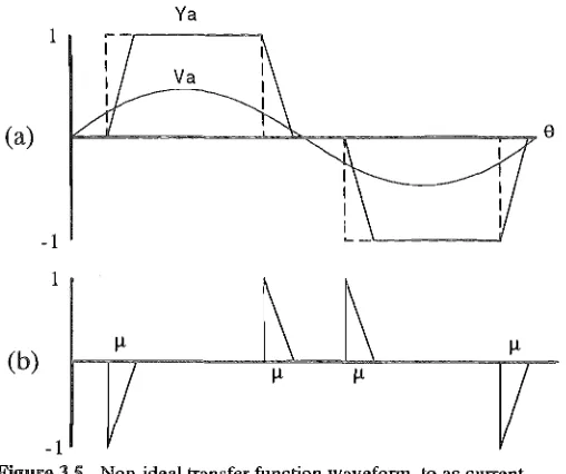
The model of [Hu and Yacamini, 1992] and [Salmi and Fujita, 1992] also provides a reasonable basis for considering convertor currents. They modelled the transfer of current from one phase to the next during the commutation period as a linear process, and applied it to a 6 pulse convertor with a steady firing angle. It is possible to express the commutation period current changeover more accurately, but the variable shape of the current transfer makes the model much more complex. This approximation is considered acceptable at this stage.

The dashed line in figure 3.5(a) represents the unmodulated ideal transfer function, and the solid line the function revised to include the commutation process. The triangular pulses of figure 3.5(b) represent the difference between these, and is called the commutation function. When firing angle modulation is applied, the pulses of the commutation function are position modulated accordingly. The duration of the triangular pulses could be approximated by the steady state commutation period, but this means that the conduction-time area of the modelled commutation period is different to the actual commutation period conduction-time area. While the characteristic spectrum of the commutation function is most closely related to the actual duration of each commutation pulse /-Lo. the non-characteristic spectrum of the commutation function is based on this area, and a hypothetical commutation period is calculated and used to yield the same conduction-time area for the simplified shape.

(38)

com-18

CHAPTER 3 THE CONVERTOR TRANSFER FUNCTION

Va

(a)

-1

(b)

[image:38.555.167.421.54.267.2]

-1

Figure 3.5 Non-ideal transfer function waveform, to ac current.

mutation current as follows

ic(t) =

~Vc

[cos(ao) - cos(wot)]

v

2Xc

(3.19) where Vc is the phase to phase rms ac system side voltage. This leads to a transfer function correction pulse of the shape

V3NlIt

F(t)

=

1 - [cos(ao) - cos(wot)]

= - -

L...,.(±)

cos[mwot - mao - m"p]

1(" m m

2V3

00 In(mb) 1("

- -

L L(±)

cos[(m

+

nk)wot - mao

+

n(ok -

-2) -

m"p]

1(" m n=l m

2V3

00 In(mb) 1("

- -

L L(±)

cos[(m - nk)wot - mao - n(ok

+ -) -

m"p]

(39)

3.4 TIlE NON-IDEAL CONVERTOR TRANSFER FUNCTION, VARIABLE COMMUTATION PERIOD

2V3 ~ Jo(mb) 2sin[mIlO] ILo

+ --

L..,,(±)

2 cos[mwot - m(ao

+ -) -

m1/J]

1(" m m mILo 2

{2.

M₃

=

_{J( b)2' [(m+nk)JlI]}

+

_v_.J

L L(±)

n In sm 2 •

1(" In n=1 m (m+nk)ILI

ILl 1(" kILl }

kILl) - m1/J]}

2 2 2

19

(3.22) for m = 1,5,7, 11 etc. Adding this to the similarly modulated ideal transfer function (from equation 3.14) yields

2V3

~

(1- Jo(mb) Jo(mb) 2 mILo -mILO)

Y",(t)

= -

L..,,(±)

2

+

s i n ( - ) / - 2 - cos[m(wot - ao - 1/J)]

1(" m m m mJLo 2 {

2V3

=

J (mb) 2sin[(m+nk)Jllj

+

- L L ( ± )

n 2

1(" m n=l m (m

+

nk)ILl .

cos[(m

+

nk)wot - m(ao

+

~l)

+

n(Ok -

i -

k~l)

- m7jJ]}

{

2 · M3

=

J ( b) 2 . [(m-nk)Jllj

+

_v_ .J

L L(

±) n m sm 2 •

1(" m n=l m (m-nk)ILl

ILl 1(" kILl }

cos[(m - nk)wot - m(ao

+

2"") -

n(Ok

+"2 -

2 ) - m7jJ] (3.23) TIlls is the non-ideal 6 pulse convertor transfer function to ac current for a steady commutation period.

If there is no firing angle modulation, the multiplier for the characteristic frequency term collapses to (±)~ m~sin(mr)/~.

3.4 The non-ideal convertor transfer function, variable commutation

period

The next step in improving the transfer function model is to consider the effect of ac side distortion, dc side distortion, and firing angle variation on the commutation period length, and to incorporate this into the modeL. While the beginning of each commutation period is affected only by the firing angle, the end of each commutation period is affected by both the firing angle and the commutation period duration. As the position of these two points may be of equal importance to the convertor transfer functions, what modulates the duration of each commutation period must be investigated.

(40)

CHAPTER 3 TIlE CONVERTOR TRANSFER FUNCnON

period variability

[image:40.555.194.392.226.326.2]

A good example of thyristor commutation analysis can be found in [Arrillaga, 1983], and is not repeated here. However, traditional analysis doesn't allow for the presence of non-characteristic harmonics. The following analyses specifically examine the of current distortion on the dc side, voltage distortion on the ac side, and firing angle variation on the commutation period. Although commutation period variability affects the position of the end of the commutation period, the terms being derived are to be sampled at the instant of firing.

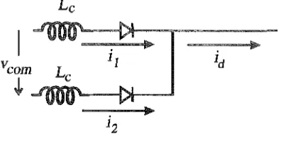
Figure 3.6 shows the circuit for a commutation analysis with distorted dc current or ac voltage. All the variables in the figure are referred to the convertor side of the convertor transformer.

Figure 3.6 The commutation circuit

From figure 3.6, two equations can be written

Vcom (3.24)

and

(3.25)

Combining these two equations yields

di2 did

vcom

=

2Lcdj - LCdt (3~6)

MUltiplying through by Wo and integrating from the time of firing

woti

to

wot,

gives

l

wot 1i2(WOt) jid(Wot)

vcomdwot = 2Xc di2 - Xc did

wot, 0 id(Woti)

(3.27)

This equation forms the basis of the commutation analysis.

3.4.1.1 current

The commutation period is directly dependent on the dc side current. If the dc current has some harmonic distortion, the commutation periods will not all be of equal length, which direct! y affects the transfer functions of the convertor. The undistorted commutation voltage is

(3.28)

(41)

3.4 THE NON-IDEAL CONVERTOR 1RANSFER FUNCTION, VARIABLE COMMUTATION PERIOD 21

The final conditions of wot

=

0:0

+

11 and i2(Wot)

=

id(wot;

+

11) are substituted in to yield

(3.30) This can be rewdtten as

(3.31 ) where the effective dc current is

(3.32)

If id is constant, equation 3.31 becomes identical to equation 3.16 dedved from a traditional commutation analysis.

To relate vadations in the commutation period to vadations in dc current, equation 3.31 can be differentiated to yield

(3.33)

To determine the full relationship it is easiest to first limit the dc side current distortion to a single frequency, as defined in equation 3.4. At any instant

(3.34) where

(3.35) The effective current over the commutation period 11 is the average of the current at the beginning and at the end of the commutation period.

I - I I coS(kwoti

+

15k)

+

coS(kwoti

+

kl1

+

15k)

dell - d

+

k 2 (3.36)

where ti is the time at the beginning of the commutation period. This can be rewritten

(3.37) This small pertubation analysis assumes that to consider the current distortion over the un-modified commutation period is sufficiently accurate, ie. that d1d(wot;) tends to O. Thus in equation 3.37 the true commutation period duration 11 is replaced by its average duration /10. This is reasonable for small levels of current distortion.

Thus the effective distortion dldel I is approximately equal to the actual distortion of the

dc current at the time of firing multiplied by cos( k~O), and phase advanced by k/1O/2 radians. Substituting this into equation 3.33 results in

dl1