Munich Personal RePEc Archive
Bootstrapping the portmanteau tests in
weak auto-regressive moving average
models
Zhu, Ke
Chinese Academy of Sciences
6 February 2015
Online at
https://mpra.ub.uni-muenchen.de/61930/
AUTO-REGRESSIVE MOVING AVERAGE MODELS
By Ke Zhu
Chinese Academy of Sciences
This paper uses a random weighting (RW) method to bootstrap the critical values for the Ljung-Box/Monti portmanteau tests and weighted Ljung-Box/Monti portmanteau tests in weak ARMA mod-els. Unlike the existing methods, no user-chosen parameter is needed to implement the RW method. As an application, these four tests are used to check the model adequacy in power GARCH models. Simulation evidence indicates that the weighted portmanteau tests have the power advantage over other existing tests. A real example on S&P 500 index illustrates the merits of our testing procedure. As one extension work, the block-wise RW method is also studied.
1. Introduction. After the seminal work of Box and Pierce (1970) and Ljung and Box (1978), the portmanteau test has been popular for diagnostic checking in the following ARMA(p, q) model:
yt= p X
i=1
φiyt−i+ q X
i=1
ψiεt−i+εt,
(1.1)
where εt is the error term withEεt = 0. Conventionally, we say that model (1.1) is
weak when{εt}is an uncorrelated sequence, and that model (1.1) is strong when{εt}
is an i.i.d. sequence; see, e.g., Francq and Zako¨ıan (1998) and Francq, Roy, and Zako¨ıan (2005). In the earlier decades, many portmanteau tests are proposed for strong ARMA models, and among them, the most famous ones are the Box-Pierce statistic Qm and
Ljung-Box statistic Qem which are defined respectively by
Qm =n m X
k=1
ˆ
ρ2k and Qme =n(n+ 2)
m X
k=1
ˆ
ρ2k n−k,
(1.2)
where n is the length of the series {yt}, m is a fixed positive integer, and ˆρk is the
residuals autocorrelation at lagk. When Eε2
t <∞, the standard analysis in Box and
Pierce (1970) or McLeod (1978) showed that the limiting distribution of Qm orQem
can be approximated byχ2
m−(p+q) in strong ARMA models, althoughQem usually has
a better finite sample performance for small n. In view of this, people more or less regard that the limiting distribution ofQmorQemis independent to the data structure
(or asymptotically pivotal in other words), and hence both test statistics can be easily
Keywords and phrases: Bootstrap method; Portmanteau test; Power GARCH models; Random weighting approach; Weak ARMA models; Weighted portmanteau test.
2
implemented in practice. Recently, Fisher and Gallagher (2012) proposed a weighted Ljung-Box statistic Qm for strong ARMA models based on the trace of the square of them-th order autocorrelation matrix, where
Qm=n(n+ 2)
m X
k=1
(m−k+ 1)
m
ˆ
ρ2k n−k.
(1.3)
Compared withQem, this new weighted Ljung-Box statistic is numerically more stable
overm, and its limiting distribution can be approximated by a gamma distribution. For more discussions on portmanteau tests in strong ARMA models, we refer to McLeod and Li (1983), Pe˜na and Rodr´ıguez (2002, 2006), Li (2004), and many others.
Although the aforementioned portmanteau tests have been well applied in indus-tries, their asymptotic properties are valid only for strong ARMA models; see, e.g., Romano and Thombs (1996). Till now, more and more empirical studies have revealed that the independence structure of error terms {εt}in model (1.1) may be restrictive especially for economic and financial series. For instance, Bollerslev (1986) used an AR(4)-GARCH(1,1) model to study the GNP series in U.S.; Franses and Van Dijk (1996) studied several stock market indexes by AR(1)-GJR(1,1) models; Zhu and Ling (2011) found that a MA(3)-GARCH(1,1) model is necessary to fit the world oil prices; see also Tsay (2005) for more empirical evidence. Moreover, Francq and Zako¨ıan (1998) and Francq, Roy, and Zako¨ıan (2005) indicated that many nonlinear models have an ARMA representation with dependent error terms. Thus, it is meaningful to consider the diagnostic checking for weak ARMA models.
So far, a huge literature has focused on testing the dependence of time series. Next, we briefly review some of important results. For the observable series, Deo (2000) con-structed some spectral tests of the martingale difference hypothesis; Lobato (2001) proposed an asymptotically pivotal test to detect whether the observable series is un-correlated; Escanciano and Velasco (2006) extended the method in Durlauf (1991) to testing the martingale difference hypothesis, taking into account both linear and non-linear dependence; Escanciano and Lobato (2009) derived a data-driven portmanteau test which is applicable in the conditionally heteroskedastic series but with no need to choose m. For the residual series, Hong and Lee (2005) considered a generalized spec-tral test which is valid for semi-strong ARMA models; Escanciano (2006) tested the martingale difference hypothesis by introducing a parametric family of functions as in Stinchcombe and White (1998); moreover, based on some marked residual processes, the Cram´er-von Mises test and Kolmogrove-Smirnov test were studied in Escanciano (2007) towards the same goal. However, none of aforementioned tests can be applied to the residuals of weak ARMA models.
used the VAR method in Berk (1974) to estimate the asymptotic covariance matrix of Qem in weak ARMA models. However, both estimation procedures have the
dis-advantage of requiring the selection of some user-chosen parameters as indicated by Kuan and Lee (2006). Moreover, they used the self-normalization method to propose a robust M test which is asymptotically pivotal and independent to user-chosen pa-rameters. This robust M test is applicable for testing serial correlations in weak AR models. Recently, Shao (2011a) proved the validity of the spectral test in Hong (1996) for detecting serial correlations in weak ARMA models. Although the spectral test is consistent, it still requires the selection of kernel function and its related bandwidth. In this paper, we bootstrap the critical values forQemandQmin weak ARMA
mod-els by a random weighting (RW) method. Unlike the existing methods, no user-chosen parameter is needed to implement this new method. Particularly, it is applicable when
εt is a martingale difference (i.e., E(εt|Ft−1) = 0 with Ft =σ(εs;s≤t)). Hence, the
RW method is valid when εthas the often observed ARCH-type structure, i.e.,
εt=ηt p
ht,
(1.4)
whereηtis i.i.d. innovation, andht∈ Ft−1 is the conditional variance ofεt. Meanwhile,
we can show that the bootstrapped critical values forQemandQmare valid for Monti’s
(1994) portmanteau test Mfm and weighted Monti portmanteau test Mm in Fisher
and Gallagher (2012), respectively, where both Mmf and Mm are based on a vector of residuals partial autocorrelations. As a byproduct, the standard deviation of m-th residuals (partial) autocorrelation can be calculated from our RW approach. Hence, the classical plot of residuals (partial) autocorrelations with the corresponding significance bounds is available for weak ARMA models. As an application, we then use all four portmanteau tests to check the adequacy of power GARCH models. Simulation studies are carried out to assess the finite-sample performance of all tests. A real example on S&P 500 index illustrates the merits of our testing procedure. As one extension work, a block-wise RW approach is also proposed to bootstrap the critical values for all tests, and its validity is justified.
This paper is organized as follows. Section 2 proposes the RW approach to bootstrap the critical values for four portmanteau tests. Section 3 applies these tests to check the model adequacy in power GARCH models. Simulation results are reported in Section 4. A real example is given in Section 5. An extension work on the block-wise RW approach is provided in Section 6. Concluding remarks are offered in Section 7. All of proofs and some additional simulation results are given in the on-line supplementary document.
2. Random weighting approach. Denote θ= (φ1,· · · , φp, ψ1,· · · , ψq)′ be the
unknown parameter of model (1.1). Let θ0 be the true value of θ and the parameter
4
Assumption 2.1. θ0 is an interior point in Θ and for each θ ∈ Θ, φ(z) , 1− Pp
i=1φizi 6= 0 and ψ(z) , 1 +Pqi=1ψizi 6= 0 when |z| ≤1, and φ(z) and ψ(z) have no common root with φp 6= 0 or ψq 6= 0.
Assumption 2.2. {yt} is strictly stationary withE|yt|4+2ν <∞ and
∞ X
k=0
{αy(k)}ν/(2+ν)<∞
for some ν >0, where {αy(k)} is the sequence of strong mixing coefficients of {yt}.
Assumption 2.1 is the condition for the stationarity, invertibility and identifiability of model (1.1). Assumption 2.2 from Francq, Roy, and Zako¨ıan (2005) gives the necessary conditions to prove our asymptotic results, and it is satisfied by many weak ARMA models, e.g.,
(a) yt=ayt−1+εt and εt=ηtηt−1;
(b) yt=aεt−1+εt and εt=ηtηt−1;
(c) yt=ηt+byt−1ηt−2,which admits a weak MA(3) representation:
yt=εt+cεt−3 as shown in Francq and Zako¨ıan (1998),
where ηt ∼N(0,1) is i.i.d. white noise, |a|<1, |b|<1, and αy(k) in each
aforemen-tioned model tends to zero exponentially fast.
Next, given the observationsχn,{y1,· · ·, yn}, we consider the least squares
esti-mator (LSE) ˆθn ofθ0, defined by
ˆ
θn= arg min Θ
˜
Ln(θ), where ˜Ln(θ) =
1
n n X
t=1
˜
ε2t(θ), 1
n n X
t=1
˜
lt(θ),
and ˜εt(θ) is defined recursively by
˜
εt(θ) =yt− p X
i=1
φiyt−i− q X
i=1
ψiε˜t−i(θ)
with ˜ε0(θ) = ˜ε−1(θ) =· · ·= ˜ε−q+1(θ) =y0 =y−1 =· · ·=y−p+1 = 0.
Denote ˆεt,ε˜t(ˆθn) be the residual of model (1.1). Then, the residuals
autocorrela-tion at lagk is
ˆ
ρk=
Pn
t=k+1εˆtεˆt−k Pn
t=1εˆ2t .
Theorem 2.1 below gives the limiting distributions ofQme in (1.2) andQmin (1.3), and under the same conditions, its proof (omitted here) follows directly from the one for Theorem 2 in Francq, Roy, and Zako¨ıan (2005). In addition, the limiting distribution ofQem in Theorem 2.1 is the same as the one in Theorem 2 of Francq, Roy, and Zako¨ıan
To state Theorem 2.1 precisely, some notations are needed. Defineεt(θ) recursively by
εt(θ) =yt− p X
i=1
φiyt−i− q X
i=1
ψiεt−i(θ),
i.e., εt(θ) =ψ−1(B)φ(B)yt, whereB is the back shift operator. Then,
∂εt(θ) ∂θ =
¡
νt−1(θ),· · · , νt−p(θ), ut−1(θ),· · ·, ut−q(θ)¢′,
where νt(θ) =−φ−1(B)εt(θ) andut(θ) =ψ−1(B)εt(θ). Particularly,εt(θ0) =εt and
∂εt ∂θ ,
∂εt(θ0)
∂θ =
∞ X
i=1 εt−iλi,
where λi = (−φ∗i−1,· · · ,−φ∗i−p, ψi−∗ 1,· · · , ψi−q∗ )′, and coefficients φ∗i and ψi∗ are from
expansions:φ−1(z) =P∞i=0φ∗izi and ψ−1(z) =P∞i=0ψ∗izi with φ∗i =ψ∗i = 0 fori <0. Moreover, letσ2 =Eε2t and define the following matrixes:
I = 4 lim
n→∞
1
nE Ã n
X
t=1 n X
t′=1
εtεt′
∂εt ∂θ
∂εt′
∂θ′ !
= 4
∞ X
i=1 ∞ X
j=1
Γ(i, j)λiλ′j,
J = 2 lim
n→∞
1
nE Ã n
X
t=1 ∂εt
∂θ ∂εt ∂θ′
!
= 2σ2 ∞ X
i=1 λiλ′i,
Rm = (Rij)1≤i, j≤m withRij =σ−4Γ(i, j),
Sm = (s1,· · · , sm) with sk = ∞ X
i=1 Rikλi,
Λm= (λ1,· · ·, λm), and
Σ =Rm+ Λ′mJ−1IJ−1Λm−2σ2Λ′mJ−1Sm−2σ2Sm′ J−1Λm,
(2.1)
where
Γ(l, l′) =
∞ X
h=−∞
E(εtεt−lεt+hεt+h−l′).
(2.2)
Here, Γ(l, l′) is meaningful by Assumptions 2.1-2.2 and Lemma A.1 in Francq, Roy, and Zako¨ıan (2005), and it satisfies Γ(l, l′) = Γ(−l,−l′) = Γ(−l′,−l). Note that Σ is
the same as Σρˆm in Theorem 2 of Francq, Roy, and Zako¨ıan (2005).
Theorem 2.1. Suppose that Assumptions 2.1-2.2 hold and model (1.1) is weak and correctly specified. Then, (i)
√
6
where →d denotes the convergence in distribution, ρˆ= (ˆρ1,· · · ,ρmˆ )′, the matrix Σ is defined in (2.1), and
W =diag ½
1,q(m−1)/m,q(m−2)/m,· · · ,q1/m ¾
is a diagonal matrix; (ii) furthermore, it follows that
e Qm →d
m X
i=1
˜
ξmiZi2 and Qm →d m X
i=1
¯
ξmiZi2 as n→ ∞,
where Z1,· · ·, Zm are independent N(0,1) variables, ξ˜m = ( ˜ξm1,· · ·,ξ˜mm)′ is the eigenvalues vector of the matrixΣ, andξm¯ = ( ¯ξm1,· · ·,ξmm¯ )′ is the eigenvalues vector of the matrix WΣW.
Remark 2.1. By using a consistent estimate Σˆ of Σ, it may be more natural to construct the test statistic nρˆ′Σˆ−1ρˆ, which has an asymptotic distribution χ2
m from Theorem 2.1. This test statistic is calculable if Σ is non singular. However, as shown in Francq, Roy, and Zako¨ıan (2005), Σ may be (or close to) singular in some cases. To overcome this difficulty, Francq, Roy, and Zako¨ıan (2005) used the spectral decom-position to express the limiting distribution ofQem, while Duchesne and Francq (2008) used the generalized inverses and{2}-inverses ofΣto construct the portmanteau test. In this paper, both methods are valid, and we follow the method in Francq, Roy, and Zako¨ıan (2005) for simplicity.
Remark 2.2. When yt follows a strong ARMA model, McLeod (1978) proved that the limiting distribution of Qem can be approximated by a χ2m−(p+q) distribution, and Fisher and Gallagher (2012) proved that the limiting distribution of Qm can be approximated by a Gamma(a, b) distribution with
a= 3 4
m(m+ 1)2
2m2+ 3m+ 1−6m(p+q) andb=
2 3
2m2+ 3m+ 1−6m(p+q)
m(m+ 1) .
(2.3)
However, simulation studies in Section 4 showed that these approximations will lead to an over-rejection problem in weak ARMA models.
From Theorem 2.1, we know that both statisticsQemandQmare applicable when Σ
can be consistently estimated. This is usually accomplished by either the kernel-based method in Newey and West (1987) or the VAR method in Francq, Roy, and Zako¨ıan (2005). However, both methods require picking up some user-chosen parameters, and hence it turns out that the testing results are sensitive to these user-chosen parameters; see, e.g., Kuan and Lee (2006). In this section, we now introduce a random weighting (RW) approach to bootstrap the critical values for Qem and Qm. This novel method
step 1. Generate a sequence of positive i.i.d. random weights {w∗1,· · ·, wn∗}, inde-pendent of the data, from a common distribution with mean and variance both equal to 1, and then calculate ˆθ∗
n via
ˆ
θn∗ = arg min
Θ
˜
L∗n(θ), where ˜L∗n(θ) = 1
n n X
t=1
w∗t˜lt(θ);
step 2. Calculate ∆ =W∗[√n(ˆρ∗−ρˆ)] with ˆρ∗ = (ˆρ∗1,· · · ,ρˆ∗m)′, where
ˆ
ρ∗k=
Pn
t=k+1w∗tεˆ∗tεˆ∗t−k Pn
t=1εˆ∗t2
with ˆε∗t = ˜εt(ˆθn∗), and the diagonal matrix
W∗ =
(
Im orWf∗ forQem W orW∗ forQm ,
(2.4)
where Im∈ Rm×m is the identity matrix,
f
W∗=diag
s n+ 2
n−1,
s n+ 2
n−2,· · · ,
s n+ 2
n−m ,
and
W∗=diag
s n+ 2
n−1,
s n+ 2
n−2
m−1
m ,· · ·, s
n+ 2
n−m
1
m ;
step 3. Repeat steps 1-2 J times to get {∆(1),· · · ,∆(J)}, and then compute its
sample variance-covariance matrix Σ∗; furthermore, simulate N i.i.d. random
sam-ples {z1(j),· · ·, zm(j)}Nj=1 from the multivariate normal distribution N(0, Im), and then
calculate the sequence{K(j)}Nj=1 via
K(j)=
m X
i=1
ξmi∗ z(ij),
where (ξm∗1,· · ·, ξ∗mm)′ is the eigenvalues vector of the matrix Σ∗;
step 4. Chooseα upper percentage of {K(j)}Nj=1 as the critical value of Qem orQm
at any given significance level α.
Particularly, when p=q= 0, we set ˆεt= ˆε∗t =yt for all tin step 2. The p-value of
e
Qm orQm can be calculated by #(K(j) >Qem)/N or #(K(j) > Qm)/N, respectively.
8
and Ling (2015). Second, the random weight wt∗ can from the standard exponential distribution as used in Section 4, the Bernoulli distribution such that
P Ã
wt∗= 3−
√
5 2
!
= 1 +
√
5
2√5 and P
Ã
w∗t = 3 +
√
5 2
!
=
√
5−1 2√5 ,
and many others. Although theoretically it is unknown how sensitive is the RW method to the distribution of w∗t, simulation studies in the on-line supplementary document imply that our testing results are robust to the distribution of w∗t. Third, although
Im and Wf∗ (or W and W∗) are close to each other when n is large, we expect that
the finite sample performance ofQem (orQm) based onWf∗ (orW ∗
) may be better for small n.
To justify the validity of the bootstrapped critical value from the RW method, two more assumptions are needed:
Assumption 2.3. E(wt∗)2+κ0 <∞ for someκ0 >0.
Assumption 2.4. For l, l′ ≥1,
∞ X
h=−∞,h6=0
E(εtεt−lεt+hεt+h−l′) = 0.
Assumption 2.3 gives one mild condition forwt∗. Assumption 2.4 restricts the depen-dent structure ofεt, and it is equivalent to say that the infinite series Γ(l, l′) in (2.2)
collapses to just one summand with the indexh= 0 (i.e.,E(ε2tεt−lεt−l′)). Particularly,
when εt is a martingale difference including the special case as in (1.4), we know that
Assumption 2.4 holds. To capture the dependence structure ofεt beyond Assumption
2.4, a block-wise technique is necessary, and we will study it in Section 6. We now are ready to state our main result:
Theorem 2.2. Suppose that Assumptions 2.1-2.4 hold and model (1.1) is weak and correctly specified. Then, conditional on χn,
√
n(ˆρ∗−ρˆ)→dN(0,Σ) in probability
as n→ ∞, where Σ is defined in (2.1).
Remark 2.3. By Theorem 2.2, it follows that conditional onχn,
f
W∗[√n(ˆρ∗−ρˆ)]→dN(0,Σ) andW ∗
[√n(ˆρ∗−ρˆ)]→dN(0, WΣW)
In the end, we show that our RW method can be also used for the portmanteau test
f
Mm in Monti (1994) and the weighted portmanteau testMm in Fisher and Gallagher
(2012), where
f
Mm=n(n+ 2) m X
k=1
ˆ
πk2
n−k and Mm =n(n+ 2) m X
k=1
(m−k+ 1)
m
ˆ
πk2 n−k
with ˆπk being the residuals partial autocorrelation at lagk. Here, ˆπk is calculated by
the Durbin-Levinson algorithm as follows:
ˆ
πk=
ˆ
ρk−(ˆρ1,· · ·,ρk−ˆ 1) ˆRk−−11(ˆρk−1,· · ·,ρˆ1)′
1−(ˆρ1,· · ·,ρˆk−1) ˆRk−−11(ˆρ1,· · ·,ρˆk−1)′ ,
where ˆRk= (ˆρ|i−j|)i,j=1,2,···,kis the Toeplitz matrix. As for Theorem 2.1, we can easily
show that √nπˆk =√nρˆk+op(1), and hence the following theorem is straightforward:
Theorem 2.3. Suppose that the conditions in Theorem 2.1 hold. Then, (i)
√
nπˆ →dN(0,Σ) and W(√nπˆ)→dN(0, WΣW) as n→ ∞,
where πˆ = (ˆπ1,· · ·,πˆm)′; (ii) furthermore, it follows thatMfm andMm have the same liming distributions as Qem and Qm, respectively.
Remark2.4. Besides the portmanteau tests aforementioned, the kernel-based spec-tral test Hn in Hong (1996) has also been widely used for testing series correlations of {εt} in model (1.1), where
Hn=
n−X1
j=1
[k(j/pn)]2ρˆ2j
withk(·)being the kernel function andpn(>0)being the bandwidth. Whenk(·)satisfies Assumption 2.1 in Shao (2011a) and pn satisfies the condition that logn=o(pn) and pn=o(n1/2), Shao (2011a) proved that if model (1.1) is weak and correctly specified,
nHn−pnC(k) p
2pnD(k) →dN(0,1) as n→ ∞, (2.5)
10
¯
p; when εt in model (1.1) is a martingale difference with conditional heteroscedasticity of unknown form, Hong and Lee (2005) re-studied this plug-in method; however, when model (1.1) is weak, how to construct and theoretically study a good data-driven method for Hn is still an open question, and we leave it for future study.
Note that the limiting distribution of√nπˆis the same as the one of√nρˆ. Thus, when model (1.1) is strong, the limiting distribution ofMmf (orMm) can be approximated
by aχ2m−(p+q)(or Gamma(a, b)) distribution as in Remark 2.2, but when model (1.1) is weak, the bootstrapped critical values forQem and Qm should be used for Mfm and Mm, respectively. In addition, it is worth noting that the standard deviation of ˆρi (or
ˆ
πi), denoted by sdi, can be calculated by
sdi = q
Σ∗ ii/n,
where Σ∗
ii is thei-th main diagonal entry of Σ∗ fori= 1,2,· · · , m. Consequently, the
classical plot of residuals (partial) autocorrelations with the corresponding significance bounds are available in weak ARMA models, where the significance lower and upper bounds for ˆρi(or ˆπi) at levelαare Φ−1[(1−α)/2]sdiand Φ−1[(1+α)/2]sdi, respectively.
Here, Φ−1(·) is the inverse of the cdf of N(0,1) distribution. As shown in Romano and Thombs (1996), the traditional significance bounds for strong ARMA models are misleading when{εt}in model (1.1) are dependent. Our significance bounds generated from the RW method are now valid for weak ARMA models, and hence they are practically important. We will illustrate this by one real example in Section 5.
3. Model checking in Power GARCH models. Since Engle (1982), ARCH-type models have become the most important tools to modeling economic and financial data sets. The power GARCH model as one of ARCH-type models describes that the power of conditional volatility depends on the past information and changes over time. Specifically, the power GARCH(r, s) (denoted by PGARCH(r, s)) model is defined as
yt=ηt p
ht and h
δ
2
t =w+ r X
i=1
αi|yt−i|δ+ s X
i=1 βih
δ
2 t−i,
(3.1)
where δ >0, w > 0, αi ≥ 0, βi ≥0, and ηt is i.i.d. innovation with mean zero and variance one. Model (3.1) as a special case of the asymmetric power GARCH models introduced by Ding, Granger, and Engle (1993) was first proposed by Higgins and Bera (1992). When δ = 2, model (3.1) reduces to the GARCH model in Bollerslev (1986), and when δ = 1, it reduces to the absolute value GARCH model in Taylor (1986) and Schwert (1989). For more discussions on ARCH-type models, we refer to Bollerslev, Chou, and Kroner (1992) and Francq and Zako¨ıan (2010).
rare. In the sequel, we briefly review some related works. Li and Mak (1994) proposed a portmanteau test to detect the adequacy of GARCH models based on the squared residuals{ηˆ2
t}; Carbon and Francq (2011) extended their work to detect the adequacy
of asymmetric PGARCH models; Li and Li (2005) considered the model checking in GARCH models by using the absolute residuals {|ηˆt|}; see also Li and Li (2008) and
Chen and Zhu (2015) for other portmanteau tests in GARCH models. In this section, we applyQem,Qm,Mfm, and Mm to check the adequacy of model (3.1).
Assume that τ , (E|ηt|δ)1/δ(> 0) is well defined. Then, we can re-parameterize
model (3.1) as
yt=ηt∗ q
h∗ t, (h∗t)
δ
2 =w∗ 1+
r X
i=1
α∗i|yt−i|δ+ s X
i=1
βi(h∗t−i)
δ
2,
(3.2)
wherew∗
1 =wτ−δ,α∗i =αiτ−δ, andηt∗=ηtτ−1. Moreover, by (3.2), a direct calculation
gives us that
|yt|δ =w∗1+
max(Xr,s)
i=1
(α∗i +βi)|yt−i|δ+vt− s X
i=1 βivt−i,
(3.3)
where we setα∗
i = 0 ifi > randβi = 0 ifi > s, andvt= (h∗t)
δ
2(|η∗
t|δ−1) is a martingale
difference. From (3.3), we know that if model (3.1) is well specified, the mean-adjusted series ˜yt,|yt|δ−E|yt|δ admits a weak ARMA(max(r, s),s) representation:
˜
yt=
max(Xr,s)
i=1
˜
αiy˜t−i+vt− s X
i=1 βivt−i,
(3.4)
where ˜αi =α∗i+βi. Thus, we can check the adequacy of model (3.1) byQem,Qm,Mfm,
andMm, which are calculated from model (3.4). Denote ˜α(z),1−Pmax(i=1 r,s)α˜izi and β(z),1−Psi=1βizi. We have the following corollary:
Corollary 3.1. Suppose that (i) Assumption 2.1 holds withφ(z)and ψ(z)being replaced byα˜(z)andβ(z), respectively; (ii) Assumption 2.2 holds withytbeing replaced by y˜t. Then, if model (3.1) is correctly specified, the conclusions in Theorems 2.1 and 2.3 hold, where Qem, Qm, Mfm, andMm are calculated from model (3.4).
12
4. Simulation study. In this section, we examine the finite-sample performance of Qem,Qm,Mfm and Mm. For Qem, we denote it by Qe(1)m , when we choose its critical
value to be the upper percentage of χ2
m−(p+q) as in strong ARMA models, while we
denote it by Qe(2)m (or Qe(3)m ), when we choose its critical value to be the one from the
RW method with W∗ =I
m (or Wf∗ as in (2.4)). ForQm, we denote it by Q (1) m , when
we choose its critical value to be the upper percentage of Gamma(a, b) as in (2.3), while we denote it by Q(2)m (or Q(3)m ), when we choose its critical value to be the one from the RW method withW∗ =W (orW∗ as in (2.4)). Likewise, we can defineMf(i) m
and M(mi) for i= 1,2,3. In all calculations, we set the significance level α = 5% and the bootstrap sample size J = 500, and generate random weights from the standard exponential distribution. In addition, more simulation studies are given in the on-line supplementary document.
4.1. Study on fitted weak ARMA models. In this subsection, we assess the finite-sample performance ofQme ,Qm,Mmf andMmon testing the model adequacy in weak
ARMA models. As a comparison, we also consider the spectral test in Hong (1996) and the robustM test (denoted byKLm) in Kuan and Lee (2006). For Hong’s
kernel-based spectral testHn, we denote it byHB(1),H (2)
B , andH (3)
B , when we use the Bartlett
kernel with the bandwidth pn=⌊3n0.3⌋,⌊9n0.3⌋, and ⌊12n0.3⌋, respectively (see, e.g.,
Kuan and Lee (2006)). Likewise, we can define HD(i), HP(i), and HQ(i) for i = 1,2,3, when we use the Daniell, Parzen, and Quadratic kernels, respectively.
In size simulations, we generate 1000 replications of sample size n= 100 and 500 from the following model:
yt= 0.9yt−1+εt, εt=ηt p
ht and ht= 1 + 0.4ε2t−1,
(4.1)
where{ηt}is a sequence of i.i.d.N(0,1) random variables. Table 1 reports the
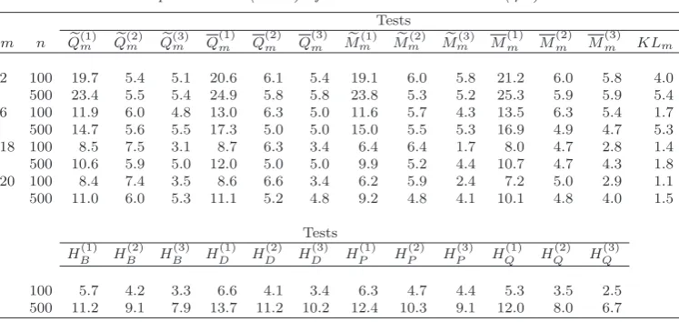
empir-ical sizes for all tests. From this table, our findings are as follows:
(ai) Qe(1)m ,Q(1)m , Mfm(1) or M(1)m has a severe over-rejection problem for each m, and
hence the critical values taken for strong ARMA models are not valid for weak ARMA models.
(aii) When nis small, the sizes of KLm become more conservative as m becomes
larger, while the sizes ofQe(2)m ,Q(2)m ,Mf (2)
m orM(2)m tend to be larger than their nominal
ones in general. In this case, the sizes of Qe(3)m , Q(3)m ,Mfm(3) or M(3)m are close to their
nominal ones, although they tend to be conservative for large m.
(aiii) Whennis large, the sizes of KLm still have a severe conservative problem for
large m. In this case, the sizes of Qe(2)m ,Q(2)m ,Mf (2)
m orM(2)m are close to their nominal
ones for each m, while the sizes of Qe(3)m , Q(3)m ,Mf (3)
m orM(3)m are slightly conservative
for largem.
Table 1
Empirical sizes (×100) of all tests based on model (4.1).
Tests m n Qe(1)m Qe(2)m Qe(3)m Q
(1) m Q
(2) m Q
(3) m Me
(1)
m Mem(2) Mem(3) M (1) m M
(2) m M
(3) m KLm
2 100 19.7 5.4 5.1 20.6 6.1 5.4 19.1 6.0 5.8 21.2 6.0 5.8 4.0
500 23.4 5.5 5.4 24.9 5.8 5.8 23.8 5.3 5.2 25.3 5.9 5.9 5.4
6 100 11.9 6.0 4.8 13.0 6.3 5.0 11.6 5.7 4.3 13.5 6.3 5.4 1.7
500 14.7 5.6 5.5 17.3 5.0 5.0 15.0 5.5 5.3 16.9 4.9 4.7 5.3
18 100 8.5 7.5 3.1 8.7 6.3 3.4 6.4 6.4 1.7 8.0 4.7 2.8 1.4
500 10.6 5.9 5.0 12.0 5.0 5.0 9.9 5.2 4.4 10.7 4.7 4.3 1.8
20 100 8.4 7.4 3.5 8.6 6.6 3.4 6.2 5.9 2.4 7.2 5.0 2.9 1.1
500 11.0 6.0 5.3 11.1 5.2 4.8 9.2 4.8 4.1 10.1 4.8 4.0 1.5
Tests
HB(1) HB(2) HB(3) HD(1) HD(2) H(3)D HP(1) HP(2) HP(3) HQ(1) HQ(2) HQ(3)
100 5.7 4.2 3.3 6.6 4.1 3.4 6.3 4.7 4.4 5.3 3.5 2.5
500 11.2 9.1 7.9 13.7 11.2 10.2 12.4 10.3 9.1 12.0 8.0 6.7
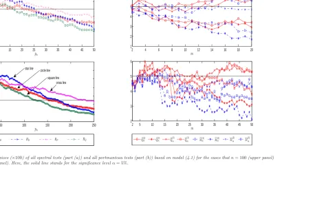
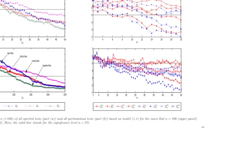
1 plots the sizes ofHB,HD,HP, andHQin the cases thatpn= 2,3,· · ·,⌊n/2⌋. As a comparison, the sizes of the portmanteau testsQe(mi),Q(mi),Mfm(i), andM(mi)(fori= 2,3)
are also plotted in the cases that m = 2,3,· · · ,20 when n= 100 or m= 2,3,· · · ,50 whenn= 500. From Figure 1, we find that for every choice of the kernel function, the sizes of the spectral test can suffer a severe over-rejection problem under a very wide range of pn, especially when n is large, while the sizes of all portmanteau tests have a robust size performance over m. This indicates that a good data-driven method for selecting pn is very important for the application of Hong’s spectral tests.
Therefore, all of these imply that the portmanteau tests along with the bootstrapped critical values from the RW method have a good size performance, while the size performance of the kernel-based spectral test in Hong (1996) heavily depends on the choice of the kernel function and related bandwidth. Particularly, we recommendQe(2)m , Q(2)m ,Mfm(2)orM(2)m for largen, andQe(3)m ,Q(3)m ,Mfm(3)orM(3)m for smallnin applications.
Next, in power simulations, we generate 1000 replications of sample size n = 100 and 500 from the following model:
yt= 0.9yt−1+ 0.2εt−1+εt, εt=ηt p
ht and ht= 1 + 0.4ε2t−1,
(4.2)
where {ηt} is a sequence of i.i.d. N(0,1) random variables. For each replication, we fit it by an AR(1) model, and then use all tests to check the adequacy of this fitted model. Table 2 reports the empirical power for all tests. Since the sizes of Qe(1)m ,Q(1)m ,
f
Mm(1),M(1)m ,HB(i),H (i) D , H
(i)
P , andH (i)
Q (fori= 1,2,3) are severely distorted in Table
1, the power of these tests in Table 2 has been adjusted by the size-correction method in Francq, Roy, and Zako¨ıan (2005, p.541) (that is, for each testTnwith a severe size distortion, its critical value used for model (4.2) is chosen as the α upper percentage of {Tni}1000i=1 , where Tni is the value of Tn for the i-th replication from model (4.1)).
14
2 5 10 15 20 25 30 35 40 45 50
0 2 4 6 8
pn
(a) Empirical sizes (× 100) of all spectral tests based on model (4.1)
2 50 100 150 200 250
0 2 4 6 8 10 12 14
pn
HB HD HP HQ
circle line
square line cross line star line
2 4 6 8 10 12 14 16 18 20
1 2 3 4 5 6 7
m
(b) Empirical sizes (× 100) of all portmanteau tests based on model (4.1)
2 5 10 15 20 25 30 35 40 45 50
2 3 4 5 6
m
e
Q(2)m Qe(3)m Q
(2)
m Q
(3)
m Mf
(2)
m Mf(3)m M
(2)
m M
(3)
m
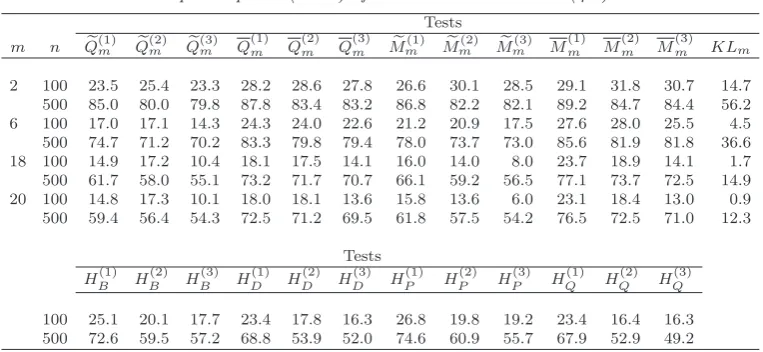
[image:15.595.121.693.113.461.2]Table 2
Empirical power (×100) of all tests based on model (4.2).
Tests m n Qe(1)m Qe(2)m Qe(3)m Q
(1) m Q
(2) m Q
(3) m Me
(1)
m Mem(2) Mem(3) M (1) m M
(2) m M
(3) m KLm
2 100 23.5 25.4 23.3 28.2 28.6 27.8 26.6 30.1 28.5 29.1 31.8 30.7 14.7
500 85.0 80.0 79.8 87.8 83.4 83.2 86.8 82.2 82.1 89.2 84.7 84.4 56.2
6 100 17.0 17.1 14.3 24.3 24.0 22.6 21.2 20.9 17.5 27.6 28.0 25.5 4.5
500 74.7 71.2 70.2 83.3 79.8 79.4 78.0 73.7 73.0 85.6 81.9 81.8 36.6
18 100 14.9 17.2 10.4 18.1 17.5 14.1 16.0 14.0 8.0 23.7 18.9 14.1 1.7
500 61.7 58.0 55.1 73.2 71.7 70.7 66.1 59.2 56.5 77.1 73.7 72.5 14.9
20 100 14.8 17.3 10.1 18.0 18.1 13.6 15.8 13.6 6.0 23.1 18.4 13.0 0.9
500 59.4 56.4 54.3 72.5 71.2 69.5 61.8 57.5 54.2 76.5 72.5 71.0 12.3
Tests
HB(1) HB(2) HB(3) HD(1) HD(2) H(3)D HP(1) HP(2) HP(3) HQ(1) HQ(2) HQ(3)
100 25.1 20.1 17.7 23.4 17.8 16.3 26.8 19.8 19.2 23.4 16.4 16.3
500 72.6 59.5 57.2 68.8 53.9 52.0 74.6 60.9 55.7 67.9 52.9 49.2
(bi) As we expected, the power of all tests becomes large as n increases, and the power of all portmanteau tests becomes small as m increases. Moreover, the power performance of Ljung-Box-type portmanteau tests and Monti-type portmanteau tests is generally comparable, while the weighted portmanteau test is more powerful than the corresponding un-weighted one, and this power advantage grows as m increases.
(bii) When n is small, Qe(2)m ,Q(2)m , Mf (2)
m or M(2)m is more powerful than Qe (3) m , Q(3)m , f
Mm(3) orM(3)m , respectively, while this power advantage disappears asnbecomes large.
This is probably becauseQe(3)m ,Q(3)m ,Mfm(3) orM(3)m has a conservative size for small n.
Moreover, the adjusted portmanteau testQe(1)m ,Q(1)m ,Mf (1)
m orM(1)m has a similar power
asQe(mi),Q(mi),Mfm(i) orM(mi), respectively, fori= 1,2, especially whennis large. This is
reasonable because all of them are based on the same statistic, and the size-correction method becomes more accurate when nis larger.
(biii) For KLm, its power is not satisfactory whenn is small and m is large. Like
portmanteau tests, its power becomes smaller as m becomes larger.
(biv) For Hong’s spectral test, its power performance varies significantly in terms of kernel function and related bandwidth. To look for further evidence, Figure 2 plots the power of HB,HD,HP, andHQ, and as a comparison, the power of the portmanteau tests Qe(mi), Q(mi), Mfm(i), and M(mi) (for i= 2,3) is also plotted in this figure. Here, the
choices ofpnandmare the same as those for Figure 1. From Figure 2, we find thatHB
and HP have a similar power performance, and they are more powerful than HD and HQ, especially when n is large. Moreover, we can see that the power of all spectral
tests generally tends to be smaller as pn becomes larger. Compared with weighted portmanteau tests, the spectral tests exhibit a dominated power advantage only when
pn is close to 2 and m is greater than 30 in the case that n = 500; however, when pn>50 in the case thatn= 500,HDandHQare much less powerful than the weighted
16
2 5 10 15 20 25 30 35 40 45 50
15 20 25 30 35
pn
(a) Empirical power (×100) of all spectral tests based on model (4.2)
2 50 100 150 200 250
30 40 50 60 70 80 90
pn
HB HD HP HQ
circle line star line
square line cross line
2 4 6 8 10 12 14 16 18 20
5 10 15 20 25 30 35
m
(b) Empirical power (×100) of all portmanteau tests based on model (4.2)
2 5 10 15 20 25 30 35 40 45 50 30
40 50 60 70 80 90
m
e
Q(2)m Qe(3)m Q
(2)
m Q
(3)
m Mf
(2)
m Mfm(3) M
(2)
m M
(3)
m
[image:17.595.115.696.115.461.2]case thatn= 100 andpn<50 in the case thatn= 500) can be much more powerful than the un-weighted portmanteau tests with a large m.
Overall, based on the bootstrapped critical values, the portmanteau tests, especially the weighted ones, give us a good indication in diagnostic checking of weak ARMA models, while the size/power performance of the spectral test is sensitive to the choice of kernel function and related bandwidth, and hence the spectral test urgently calls for a good data-driven method for selecting the bandwidth.
4.2. Study on fitted PGARCH models. In this subsection, we examine the finite-sample performance of Qem,Qm, Mfm and Mm on testing the adequacy of PGARCH
models. As a comparison, we also consider the portmanteau test QCFm in Carbon and Francq (2011). In size simulations, we generate 1000 replications of sample size
n= 1000 from the following model:
yt=ηt p
ht, h
δ
2
t = 0.2 + 0.2|yt−1|δ,
(4.3)
where{ηt}is a sequence of i.i.d.N(0,1) random variables. Table 3 reports the results for the size study. From Table 3, we find that in general, the sizes of all tests are close to their nominal ones, while the sizes ofQem,Qm,MfmandMmseem to be conservative
when both δ and m are large.
Table 3
Empirical sizes (×100) of all tests based on model (4.3).
Tests
δ m Qem Qm Mem Mm QCFm
2.5 6 4.9 5.5 4.9 5.7 2.7
12 2.6 4.0 2.8 4.3 3.1
24 1.7 2.1 2.0 2.3 2.6
32 0.9 1.6 1.5 1.9 3.3
2.0 6 3.5 4.8 3.9 4.6 2.6
12 3.3 4.3 3.3 4.3 2.9
24 2.1 2.6 2.1 2.7 4.0
32 2.3 2.3 2.3 2.4 3.7
1.0 6 7.3 7.2 7.1 6.5 6.6
12 6.5 7.3 6.3 6.5 8.3
24 5.4 6.6 4.8 6.2 6.7
32 5.8 5.9 5.1 5.5 7.4
0.5 6 5.4 5.6 5.4 5.6 3.5
12 6.3 5.0 6.0 5.2 4.1
24 5.2 6.1 5.4 5.3 4.1
32 5.0 5.7 5.2 5.8 3.4
Next, in power simulations, we generate 1000 replications of sample size n= 1000 from the following model:
yt=ηt p
ht, h
δ
2
t = 0.2 + 0.2|yt−1|δ+ 0.2|yt−2|δ,
(4.4)
where {ηt} is a sequence of i.i.d. N(0,1) random variables. For each replication, we
18
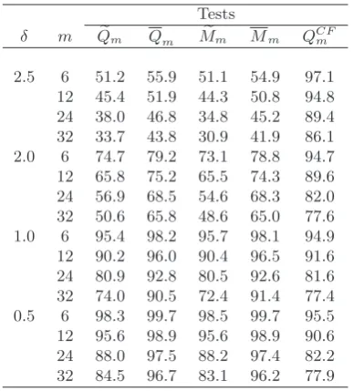
portmanteau tests to check the adequacy of this fitted model. Table 4 reports the results for the power study, where the critical values for Qem, Qm, Mfm or Mm are
chosen as forQe(2)m ,Q(2)m ,Mf (2)
m orM(2)m , respectively. From Table 4, we find that whenδ
is small, the weighted testsQmandMmare more powerful than others. However, when δis large,QCF
m is the best performing test statistic. Overall, our weighted portmanteau
tests have a good performance especially when δ is small.
[image:19.595.191.391.209.424.2]Table 4
Empirical power (×100) of all tests based on model (4.4).
Tests
δ m Qem Qm Mem Mm QCFm
2.5 6 51.2 55.9 51.1 54.9 97.1 12 45.4 51.9 44.3 50.8 94.8 24 38.0 46.8 34.8 45.2 89.4 32 33.7 43.8 30.9 41.9 86.1 2.0 6 74.7 79.2 73.1 78.8 94.7 12 65.8 75.2 65.5 74.3 89.6 24 56.9 68.5 54.6 68.3 82.0 32 50.6 65.8 48.6 65.0 77.6 1.0 6 95.4 98.2 95.7 98.1 94.9 12 90.2 96.0 90.4 96.5 91.6 24 80.9 92.8 80.5 92.6 81.6 32 74.0 90.5 72.4 91.4 77.4 0.5 6 98.3 99.7 98.5 99.7 95.5 12 95.6 98.9 95.6 98.9 90.6 24 88.0 97.5 88.2 97.4 82.2 32 84.5 96.7 83.1 96.2 77.9
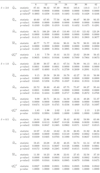
5. A real example. In this section, we revisit the real example on S&P 500 index in Francy, Roy, and Zako¨ıan (2005). The data sample taken from January 3, 1979 to December 31, 2001 has in total 5808 observations, and its log-return is denoted by
{yt}5807t=1. First, we use Qem, Qm, Mfm and Mm to check whether {yt} is a sequence
of white noises. The p-value is calculated either as in strong ARMA models (denoted by p-value1) or via the RW method with J = 500 (denoted by p-value2). All testing results are reported in Table 5, from which we know that at the significance level 5%, the strong white noise hypothesis is rejected, while the weak white noise hypothesis is not rejected. This is consistent to the findings in Francy, Roy, and Zako¨ıan (2005). Next, we want to check whether a PGARCH(1,1) model in (3.1) withδ = 2.0, 1.0 or 0.5 is adequate to fit {yt}. Denote by ˜yt=|yt|δ−E|yt|δ the mean-adjusted series. As in (3.4), we obtain the following three fitted models:
Model A : ˜yt= 0.8287˜yt−1−0.7236vt−1+vt withσv2t = 5.26×10
−7 and δ= 2.0;
Model B : ˜yt= 0.9753˜yt−1−0.8979vt−1+vt withσv2t = 4.99×10
−5 and δ= 1.0;
Model C : ˜yt= 0.9920˜yt−1−0.9513vt−1+vt withσ2vt = 1.30×10
−3 and δ = 0.5.
For models A-C, we useQem,Qm,MfmandMm to check their adequacy. As a
compar-ison, we also useQCF
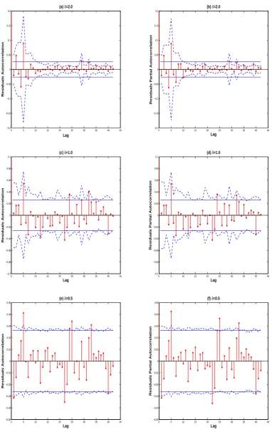
are reported in Table 6. From this table, we find that at the significance level 5%, all tests suggest that models A and B are adequate, while except QCFm , the other tests indicate that model C is not adequate. To look for further evidence, Figure 3 plots the residuals autocorrelations and partial autocorrelations for models A-C. From Figure 3, we know that the 1st, 5th, 22th, 25th and 33th residuals autocorrelations or partial autocorrelations in model C all exceed the 95% significance bounds. Thus, it suggests that model C is not adequate. Moreover, since model A has a smaller sum of squared errors than model B, we prefer to fit{yt}by a PGARCH(1,1) model withδ = 2 (i.e.,
GARCH(1,1) model). Finally, it is worth noting that although the conclusions drawn from Qem, Qm, Mfm and Mm are the same, the p-value2s of Qm or Mm tend to be
[image:20.595.131.448.308.489.2]more stable over all lags for model C. In view of this, we recommend the weighted test Qm orMm to practitioners.
Table 5
Testing results for the adequacy of a white noise on S&P 500 index.
m
6 12 18 24 30 36 42
e
Qm statistic 25.58 36.07 38.49 46.62 64.49 78.77 87.71
p-value1† 0.0003 0.0003 0.0033 0.0037 0.0003 0.0000 0.0000
p-value2§ 0.4758 0.5283 0.6874 0.6990 0.5292 0.4634 0.4518
Qm statistic 20.64 25.17 28.98 32.25 37.65 43.73 49.37
p-value1 0.0000 0.0000 0.0001 0.0002 0.0002 0.0001 0.0000
p-value2 0.3508 0.4805 0.5494 0.5967 0.5817 0.5719 0.5477
e
Mm statistic 25.06 36.39 38.78 46.63 63.75 76.68 86.08
p-value1 0.0003 0.0003 0.0033 0.0037 0.0003 0.0000 0.0000
p-value2 0.4881 0.5219 0.6833 0.6990 0.5441 0.4977 0.4776
Mm statistic 20.40 24.87 28.89 32.30 37.72 43.47 48.85
p-value1 0.0000 0.0000 0.0001 0.0002 0.0002 0.0001 0.0000
p-value2 0.3578 0.4871 0.5507 0.5941 0.5783 0.5754 0.5545
†p-values taken as in strong ARMA models.
§p-values bootstrapped by the RW method withW∗=I
m(orW) forQemandMem
(orQmandMm).
6. Block-wise random weighting approach. Although the bootstrapped crit-ical values based on the RW method are valid for weak ARMA models, the condition in Assumption 2.4 seems to be slightly restrictive in practice. In this section, we propose a block-wise RW method to obtain the bootstrapped critical values for all portmanteau tests. Our bootstrapped critical values from the block-wise RW method are valid without posing Assumption 2.4, but it requires a selection of block size as many block-wise bootstrap methods in the literature; see, e.g., Romano and Thombs (1996), Horowitz, Lobato, Nankervis, and Savin (2006), and Shao (2011b).
The detailed procedure to bootstrap the critical values by the block-wise RW method is the same as the one in steps 1-4 in Section 2, except replacing step 1 by step 1′ as follows:
step 1′. Set a block size b
20
Table 6
Testing results for the adequacy of a PGARCH(1,1) model on S&P 500 index.
m
6 12 18 24 30 36 42
δ= 2.0 Qem statistic 87.44 96.42 97.39 99.61 105.6 110.3 111.7
p-value1† 0.0000 0.0000 0.0000 0.0000 0.0000 0.0000 0.0000
p-value2§ 0.4063 0.4358 0.4416 0.4483 0.4432 0.4428 0.4246
Qm statistic 40.60 67.95 77.56 82.86 86.67 90.39 93.35
p-value1 0.0000 0.0000 0.0000 0.0000 0.0000 0.0000 0.0000
p-value2 0.4349 0.4293 0.4319 0.4431 0.4452 0.4475 0.4281
e
Mm statistic 86.51 106.20 108.45 110.80 115.93 121.02 123.28
p-value1 0.0000 0.0000 0.0000 0.0000 0.0000 0.0000 0.0000
p-value2 0.4115 0.3841 0.3845 0.3929 0.3911 0.3903 0.3677
Mm statistic 40.77 71.77 83.64 90.31 94.79 98.91 102.26
p-value1 0.0000 0.0000 0.0000 0.0000 0.0000 0.0000 0.0000
p-value2 0.4325 0.4009 0.3934 0.3995 0.3983 0.3993 0.3811
QCF
m statistic 1.44 7.79 10.44 16.53 23.62 29.08 56.45
p-value 0.9635 0.8014 0.9166 0.8680 0.7889 0.7864 0.0673
δ= 1.0 Qem statistic 22.90 39.57 46.11 67.54 76.99 94.13 101.4
p-value1 0.0001 0.0000 0.0001 0.0000 0.0000 0.0000 0.0000
p-value2 0.4497 0.4093 0.4174 0.2739 0.2839 0.2091 0.2151
Qm statistic 9.15 20.58 28.30 34.78 42.27 50.10 56.98
p-value1 0.0000 0.0000 0.0000 0.0000 0.0000 0.0000 0.0000
p-value2 0.6445 0.5258 0.4703 0.4507 0.4044 0.3553 0.3248
e
Mm statistic 22.72 38.80 45.40 67.75 75.87 88.27 95.44
p-value1 0.0001 0.0000 0.0001 0.0000 0.0000 0.0000 0.0000
p-value2 0.4544 0.4244 0.4309 0.2717 0.2966 0.2672 0.2768
Mm statistic 9.09 20.71 28.14 34.59 42.16 49.26 55.37
p-value1 0.0000 0.0000 0.0000 0.0000 0.0000 0.0000 0.0000
p-value2 0.6474 0.5219 0.4745 0.4556 0.4069 0.3723 0.3497
QCF
m statistic 1.83 1.98 2.02 2.10 2.11 2.13 2.23
p-value 0.9350 0.9994 1.0000 1.0000 1.0000 1.0000 1.0000
δ= 0.5 Qem statistic 18.64 22.86 25.07 39.42 49.92 59.99 65.88
p-value1 0.0009 0.0113 0.0687 0.0126 0.0066 0.0039 0.0061
p-value2 0.0204 0.0847 0.2465 0.0962 0.0571 0.0417 0.0515
Qm statistic 10.97 15.82 18.62 21.58 26.85 31.92 36.36
p-value1 0.0000 0.0009 0.0063 0.0149 0.0092 0.0062 0.0054
p-value2 0.0339 0.0405 0.0703 0.1090 0.0784 0.0637 0.0555
e
Mm statistic 19.45 23.08 25.30 40.35 50.74 61.14 67.90
p-value1 0.0009 0.0113 0.0687 0.0126 0.0066 0.0039 0.0061
p-value2 0.0172 0.0820 0.2385 0.0837 0.0515 0.0351 0.0389
Mm statistic 11.30 16.23 18.96 22.01 27.45 32.56 37.10
p-value1 0.0000 0.0009 0.0063 0.0149 0.0092 0.0062 0.0054
p-value2 0.0295 0.0344 0.0634 0.0985 0.0679 0.0566 0.0475
QCF
m statistic 0.0927 0.0930 0.0931 0.0934 0.0935 0.0936 0.0942
p-value 1.0000 1.0000 1.0000 1.0000 1.0000 1.0000 1.0000
†p-values taken as in strong ARMA models.
§p-values bootstrapped by the RW method withW∗=I
m(orW) forQemandMem (or
0 5 10 15 20 25 30 35 40 45 −0.2
−0.15 −0.1 −0.05 0 0.05 0.1 0.15 0.2
Lag
Residuals Autocorrelation
(a) δ=2.0
0 5 10 15 20 25 30 35 40 45 −0.2
−0.15 −0.1 −0.05 0 0.05 0.1 0.15 0.2
Lag
Residuals Partial Autocorrelation
(b) δ=2.0
0 5 10 15 20 25 30 35 40 45 −0.1
−0.08 −0.06 −0.04 −0.02 0 0.02 0.04 0.06 0.08 0.1
Lag
Residuals Autocorrelation
(c) δ=1.0
0 5 10 15 20 25 30 35 40 45 −0.1
−0.08 −0.06 −0.04 −0.02 0 0.02 0.04 0.06 0.08 0.1
Lag
Residuals Partial Autocorrelation
(d) δ=1.0
0 5 10 15 20 25 30 35 40 45 −0.05
−0.04 −0.03 −0.02 −0.01 0 0.01 0.02 0.03 0.04 0.05
Lag
Residuals Autocorrelation
(e) δ=0.5
0 5 10 15 20 25 30 35 40 45 −0.05
−0.04 −0.03 −0.02 −0.01 0 0.01 0.02 0.03 0.04 0.05
Lag
Residuals Partial Autocorrelation
[image:22.595.101.484.82.689.2](f) δ=0.5
22
{(s−1)bn+1,· · ·, sbn}fors= 1,· · ·, Ln, whereLn=n/bnis assumed to be an integer for the convenience of presentation; furthermore, generate a sequence of positive i.i.d. random variables{δ1,· · ·, δLn}, independent of the data, from a common distribution with mean and variance both equal to 1, and then define the random weightswt∗ =δs,
ift∈Bs, fort= 1· · ·, n; finally, calculate ˆθn∗ via
ˆ
θ∗n= arg min
Θ
˜
L∗n(θ), where ˜L∗n(θ) = 1
n n X
t=1
wt∗˜lt(θ).
Clearly, the block-wise RW method is a natural extension of the RW method, and the validity of the bootstrapped critical value from the block-wise RW method is justified by the following theorem:
Theorem6.1. Suppose that (i) Assumptions 2.1-2.3 hold and model (1.1) is weak and correctly specified; (ii)E|yt|8+4ν <∞for someν >0andlimk→∞k2[αy(k)]ν/(2+ν)
= 0; and (iii) limn→∞bn=∞ and limn→∞bn/n1/3= 0. Then, conditional on χn,
√
n(ˆρ∗−ρˆ)→dN(0,Σ) in probability
as n→ ∞, where Σ is defined in (2.1).
The proof of Theorem 6.1 is given in the Appendix. Here, condition (ii) poses some additional requirements onyt, and condition (iii) gives some restrictions on the
block-size bn. Both of them are necessary for the proof. From Theorem 6.1, we know that
the performance of our tests along with their critical values from the block-wise RW method depends on the user-chosen parameterbn. This may be the price we pay for not
assuming Assumption 2.4. Simulation studies in the on-line supplementary document show that our testing results are not sensitive to the user-chosen parameter bn, while
the size performance of Hong’s (1996) kernel-based spectral test is not robust to the choices of the bandwidth pn. Till now, how to select the optimal bn under certain
“criterion” is unknown. This is a familiar problem with all blocking methods. The heuristic work in Hall, Horowitz, and Jing (1995), Politis, Romano, and Wolf (1999), and Sun (2014) may be extended in this case, and we leave it for future study.
7. Concluding remarks. In this paper, by using the RW method, we bootstrap the critical values for Ljung-Box/Monti portmanteau tests Qem/Mfm and weighted
Ljung-Box/Monti portmanteau testsQm/Mm in weak ARMA models. Unlike the
method have the power advantage over the un-weighted ones in general; (ii) the sizes of all portmanteau tests are robust to the choices of the lag m, while the sizes of the kernel-based spectral tests in Hong (1996) are sensitive to the choices of the band-widthpn; and (iii) the weighted portmanteau testsQm/Mmcan be significantly more
powerful than the kernel-based spectral tests with an inappropriate choice of pn. As
one extension work, we also propose a block-wise RW method to bootstrap the critical values for all portmanteau tests, and its validity is justified.
Finally, we suggest three future subjects, which may lead to some better specifi-cation tests. First, as in Escanciano and Lobato (2009), it is of interest to consider the case that m is not fixed but optimally chosen by the data set. If it is possible, a more powerful testing procedure should be expected. Second, till now, less is known to choose the optimal weight matrix W (in some sense) such that the corresponding weighted Ljung-Box or Monti portmanteau test has the best performance among all weighted portmanteau tests in strong ARMA models. We may expect that the merits of this optimal weighted portmanteau test still hold in weak ARMA models. Third, since all portmanteau tests still need a selection ofm, they can not detect serial corre-lations beyond lagm. Hence, it is a practical demand to study the Cram´er-von Mises spectral test (e.g., Shao (2011b)) which can detect serial correlations at all lags.
Acknowledgement. I am grateful to the two referees, the Associate Editor and the Joint Editor I. Van Keilegom for very constructive suggestions and comments, lead-ing to a substantial improvement in the presentation and the elimination of two errors in the previous manuscript. This work is partially supported by National Natural Sci-ence Foundation of China (No.11201459), President Fund of Academy of Mathematics and Systems Science, CAS (No.2014-cjrwlzx-zk), and Key Laboratory of RCSDS, CAS.
References.
[1] Beltrao, K. and Bloomfield, P. (1987) Determining the bandwidth of a kernel spectrum estimate.Journal of Time Series Analysis8, 21-38.
[2] Berk, K.N.(1974) Consistent autoregressive spectral estimates.Annals of Statistics2, 489-502.
[3] Bollerslev, T. (1986) Generalized autoregressive conditional heteroskedasticity. Journal of
Econometrics31, 307-327.
[4] Bollerslev, T.,Chou, R.Y., andKroner, K.F.(1992) ARCH modeling in finance: A review of the theory and empirical evidence.Journal of Econometrics52, 5-59.
[5] Box, G.E.P. and Pierce, D.A. (1970) Distribution of the residual autocorrelations in au-toregressive integrated moving average time series models.Journal of the American Statistical
Association65, 1509-1526.
[6] Carbon, M.and Francq, C. (2011) Portmanteau goodness-of-fit test for asymmetric power GARCH models.Austrian Journal of Statistics40, 55-64.
[7] Carrasco, M. and Chen, X.(2002) Mixing and moment properties of various GARCH and stochastic volatility models.Econometric Theory18, 17-39.
24
[9] Chen, K., Ying, Z., Zhang, H., and Zhao, L. (2008) Analysis of least absolute deviation.
Biometrika95, 107-122.
[10] Chen, K., Guo, S., Lin, Y., and Ying, Z. (2010) Least absolute relative error estimation.
Journal of the American Statistical Association105, 1104-1112.
[11] Deo, R.S.(2000) Spectral tests of the martingale hypothesis under conditional
heteroskedastic-ity.Journal of Econometrics99, 291-315.
[12] Ding, Z.,Granger, C.W.J.andEngle, R.F.(1993) A long memory property of stock market returns and a new model.Journal of Empirical Finance1, 83-106.
[13] Duchesne, P.andFrancq, C.(2008) On diagnostic checking time series models with portman-teau test statistics based on generalized inverses and{2}-inverses.COMPSTAT 2008, Proceedings
in Computational Statistics, (ed.) P. Brito, Heidelberg: Physica-Verlag, pp. 143-154.
[14] Durlauf, S.N.(1991) Spectral-based testing of the martingale hypothesis.Journal of
Econo-metrics50, 355-376.
[15] Engle, R.F.(1982) Autoregressive conditional heteroskedasticity with estimates of variance of U.K. inflation.Econometrica50, 987-1008.
[16] Escanciano, J.C. (2006) Goodness-of-fit tests for linear and non-linear time series models.
Journal of the American Statistical Association101, 531-541.
[17] Escanciano, J.C. (2007) Model checks using residual marked emprirical processes.Statistica
Sinica17, 115-138.
[18] Escanciano, J.C.andVelasco, C.(2006) Generalized spectral tests for the martingale differ-ence hypothesis.Journal of Econometrics134, 151-185.
[19] Escanciano, J.C.andLobato, I.N.(2009) An automatic portmanteau test for serial correla-tion.Journal of Econometrics151, 140-149.
[20] Fisher, T.J.andGallagher, C.M.(2012) New weighted portmanteau statistics for time series goodness of fit testing.Journal of the American Statistical Association107, 777-787.
[21] Francq, C.,Roy, R., andZako¨ıan, J.M. (2005) Diagostic checking in ARMA models with uncorrelated errors.Journal of the American Statistical Association100, 532-544.
[22] Francq, C.andZako¨ıan, J.M.(1998) Estimating linear representations of nonlinear processes.
Journal of Statistical Planning and Inference68, 145-165.
[23] Francq, C. andZako¨ıan, J.M. (2010) GARCH Models: Structure, Statistical Inference and Financial Applications. Wiley, Chichester, UK.
[24] Franses, P.H.andVan Dijk, R.(1996) Forecasting stock market volatility using (non-linear) Garch models.Journal of Forecasting15, 229-235.
[25] Giot, P. and Laurent, S. (2004) Modelling daily value-at-risk using realized volatility and Arch type models.Journal of Empirical Finance11, 379-398.
[26] Hall, P., Horowitz, J.L., and Jing, B.-Y.(1995) On blocking rules for the bootstrap with dependent data.Biometrica82, 561-574.
[27] Higgins, M.L.andBera, A.K.(1992) A class of nonlinear ARCH models.International
Eco-nomic Review33, 137-158.
[28] Hong, Y. (1996) Consistent testing for serial correlation of unknown form.Econometrica 64,
837-864.
[29] Hong, Y.(1999) Hypothesis testing in time series via the empirical characteristic function: a generalized spectral density approach.Journal of the American Statistical Association94,
1201-1220.
[30] Hong, Y. and Lee, T.H. (2003) Diagnostic checking for adequacy of nonlinear time series models.Econometric Theory19, 1065-1121.
[32] Horowitz, J.L.,Lobato, I.N.,Nankervis, J.C., andSavin, N.E.(2006) Bootstrapping the Box-Pierce Q test: A robust test of uncorrelatedness.Journal of Econometrics133, 841-862.
[33] Jin, Z.,Ying, Z.andWei, L.J.(2001) A simple resampling method by perturbing the minimand.
Biometrika88, 381-390.
[34] Kuan, C.-M. and Lee, W.-M. (2006) Robust M tests without consistent estimation of the asymptotic covariance matrix.Journal of the American Statistical Association101, 1264-1275.
[35] Lee, J. and Hong, Y. (2001) Testing for serial correlation of unknown form using wavelet methods.Econometric Theory17, 386-423.
[36] Li, W.K. (1992) On the asymptotic standard errors of residual autocorrelations in nonlinear time series modelling.Biometrika79, 435-437.
[37] Li, W.K.(2004) Diagnostic checks in time series. Chapman& Hall/CRC.
[38] Li, G.,Leng, C.andTsai, C.-L.(2014) A hybrid bootstrap approach to unit root tests.Journal
of Time Series Analysis35, 299-321.
[39] Li, G.and Li, W.K. (2005) Diagnostic checking for time series models with conditional het-eroscedasticity estimated by the least absolute deviation approach.Biometrika92, 691-701.
[40] Li, G. and Li, W.K. (2008). Least absolute deviation estimation for fractionally integrated autoregressive moving average time series models with conditional heteroscedasticity.Biometrika 95, 399-414.
[41] Li, G.,Li, Y.andTsai, C.-L.(2014) Quantile correlations and quantile autoregressive modeling. Forthcoming inJournal of the American Statistical Association.
[42] Li, W.K. and Mak, T.K.(1994) On the squared residual autocorrelations in non-linear time series with conditional heteroscedasticity.Journal of Time Series Analysis15, 627-636.
[43] Ljung, G.M. and Box, G.E.P. (1978) On a measure of lack of fit in time series models.
Biometrika65, 297-303.
[44] Lobato, I.N.(2001) Testing that a dependent process is uncorrelated.Journal of the American
Statistical Association96, 1066-1076.
[45] McKenzie, M.andMitchell, H.(2002) Generalised asymmetric power arch modeling of ex-change rate volatility.Applied Financial Economics12, 555-564.
[46] McLeod, A.I.andLi, W.K.(1983) Diagnostic checking ARMA time series models using square-dresidual autocorrelations.Journal of Time Series Analysis4, 269-273.
[47] McLeod, A.I.(1978) On the distribution of residual autocorrelations in Box-Jenkins method,
Journal of the Royal Statistical SocietyB 40, 296-302.
[48] Monti, A.C.(1994) A proposal for a residual autocorrelation test in linear models.Biometrika 81, 776-780.
[49] Newey, W.K. andWest, K.D.(1987) A simple positive semi-definite heteroskedasticity and autocorrelation consistent covariance matrix.Econometrica55, 703-708.
[50] Pe˜na, D. andRodr´ıguez, J.(2002) A powerful portmanteau test of lack of fit for time series.
Journal of the American Statistical Association97, 601-610.
[51] Pe˜na, D.andRodr´ıguez, J.(2006), The Log of the determinant of the autocorrelation matrix for testing goodness of fit in time series. Journal of Statistical Planning and Inference 136,
2706-2718.
[52] Romano, J.L.andThombs, L.A.(1996) Inference for autocorrelations under weak assumptions.
Journal of the American Statistical Association91, 590-600.
[53] Politis, D.N.,Romano, J., andWolf, M.(1999)Subsampling Springer-Verla, New York. [54] Schwert, G.W.(1989) Why does stock market volatility change over time?Journal of Finance
45, 1129-1155.
[55] Shao, X.(2011a). Testing for white noise under unknown dependence and its applications to diagnostic checking for time series models.Econometric Theory27, 312-343.
26
Journal of Econometrics162, 213-224.
[57] Stinchcombe, M.andWhite, H.(1998) Consistent specification testing with nuisance param-eters present only under the alternative.Econometric Theory14, 295-325.
[58] Sun, Y.(2014) Let’s fix it: Fixed-b asymptotics versus small-b asymptotics in heteroskedasticity and autocorrelation robust inference.Journal of Econometrics178, 659-677.
[59] Taylor, S.(1986) Modelling Financial Time Series. Wiley, New York.
[60] Tsay, R.S.(2005) Analysis of Financial Time Series (2nd ed.). New York: John Wiley&Sons, Incorporated.
[61] Wu, C.F.J. (1986) Jacknife, bootstrap and other resampling methods in regression analysis (with discussion).Annals of Statistics14, 1261-1350.
[62] Zhu, K.andLing, S.(2011) Global self-weighted and local quasi-maximum exponential likeli-hood estimators for ARMA-GARCH/IGARCH models.Annals of Statistics 39, 2131-2163.
[63] Zhu, K. and Ling, S. (2015) LADE-based inference for ARMA models with unspecified and heavy-tailed heteroscedastic noises. Forthcoming inJournal of the American Statistical
Associ-ation.
Chinese Academy of Sciences Institute of Applied Mathematics Haidian District, Zhongguancun Beijing, China
AUTO-REGRESSIVE MOVING AVERAGE MODELS (SUPPLEMENTARY DOCUMENT)
By Ke Zhu
Chinese Academy of Sciences
In this supplementary material, we give some simulation studies and all of the proofs for the paper in Appendix.
1. Additional simulation studies. In this section, we give some simulation studies, which are useful but not reported in the paper. In Subsection 1.1, we check the sensitivity of the distribution of random weights to our portmanteau tests by simula-tion. In Subsection 1.2, we examine the finite-sample performance of our portmanteau tests as in Section 4 of the paper by some additional simulations. In Subsection 1.3, we assess the finite-sample performance of the block-wise RW method.
1.1. Sensitivity of the distribution of random weights. In simulation studies of the paper, we generate random weights{wt∗}from the standard exponential distribution. In this subsection, we check the sensitivity of the distribution of {w∗
t} to our port-manteau tests by generating{wt∗}from the Bernoulli distribution such that
P
Ã
wt∗= 3− √
5 2
! = 1 +
√ 5
2√5 and P Ã
w∗t = 3 + √
5 2
! =
√ 5−1 2√5 .
Table 1
Empirical sizes(×100)of all tests based on model (4.1) in the paper.
Tests m n Qe(2)m Qe(3)m Q
(2)
m Q
(3)
m Mem(2) Mem(3) M
(2)
m M
(3)
m
2 100 5.8 5.2 5.6 5.3 5.3 4.8 5.4 5.1 500 4.3 4.2 4.8 4.3 4.2 4.2 4.7 4.7 6 100 5.0 4.1 5.2 4.5 4.1 3.5 4.6 3.7 500 3.9 3.7 4.3 4.2 3.5 3.3 3.7 3.6 18 100 6.0 3.4 5.2 4.0 4.2 1.7 3.8 2.6 500 3.9 3.4 3.4 3.2 3.2 3.0 3.4 3.3 20 100 6.5 3.4 5.5 3.8 4.4 2.0 3.8 2.5 500 4.0 3.7 3.4 3.0 3.1 3.0 3.0 2.8
Tables 1-2 are obtained in the same way as Tables 1-2 in the paper. From these four tables, we can see that our testing results are robust to the distribution ofwt∗.
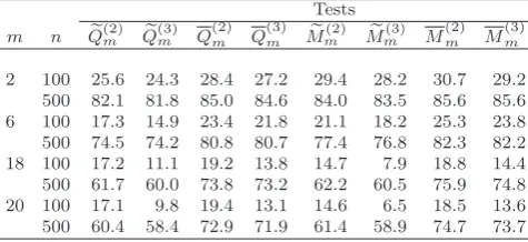
1.2. Some additional simulations. In this subsection, we examine the finite-sample performance of our portmanteau tests as in Section 4 of the paper by some additional simulations. Hereafter, we generate {wt∗}from the standard exponential distribution.
2
Table 2
Empirical power(×100)of all tests based on model (4.2) in the paper.
Tests m n Qe(2)m Qe(3)m Q
(2)
m Q
(3)
m Me
(2)
m Mem(3) M
(2)
m M
(3)
m
2 100 25.6 24.3 28.4 27.2 29.4 28.2 30.7 29.2 500 82.1 81.8 85.0 84.6 84.0 83.5 85.6 85.6 6 100 17.3 14.9 23.4 21.8 21.1 18.2 25.3 23.8 500 74.5 74.2 80.8 80.7 77.4 76.8 82.3 82.2 18 100 17.2 11.1 19.2 13.8 14.7 7.9 18.8 14.4 500 61.7 60.0 73.8 73.2 62.2 60.5 75.9 74.8 20 100 17.1 9.8 19.4 13.1 14.6 6.5 18.5 13.6 500 60.4 58.4 72.9 71.9 61.4 58.9 74.7 73.7
First, we study it for fitted weak ARMA models. In size simulations, we generate 1000 replications of sample size n= 100 and 500 from the following model:
yt= 0.9εt−1+εt, εt=ηtηt−1, (1.1)
where {ηt} is a sequence of i.i.d. N(0,1) random variables. Table 3 reports the em-pirical sizes for all tests except the robust M test, which is not valid for MA models. From Table 3, our findings are the same as those from Table 1 in the paper. Moreover, Figure 1 below plots the empirical sizes of all spectral tests and portmanteau tests, and our findings from this figure are the same as those from Figure 1 in the paper.
Table 3
Empirical sizes (×100) of all tests based on model (1.1).
Tests m n Qe(1)m Qe(2)m Qe(3)m Q
(1)
m Q
(2)
m Q
(3)
m Me
(1)
m Mem(2) Mem(3) M
(1)
m M
(2)
m M
(3)
m
2 100 17.7 5.5 4.9 20.2 6.4 5.9 18.1 6.7 6.1 21.1 6.3 6.2 500 29.6 6.2 6.1 29.6 6.6 6.5 25.7 6.6 6.4 29.6 7.2 6.9 6 100 8.9 4.6 3.8 10.6 5.9 5.0 10.0 5.2 4.8 11.1 6.4 5.2 500 14.5 5.1 4.9 17.7 6.3 6.3 14.5 5.6 5.5 17.2 6.4 6.3 18 100 7.2 5.3 2.1 6.7 5.2 3.3 6.3 4.8 2.4 7.2 5.1 3.5 500 10.2 3.6 3.3 11.7 5.2 4.7 9.6 4.3 4.0 11.7 4.8 4.7 20 100 6.1 5.8 2.1 6.9 5.3 2.7 5.0 4.7 2.2 6.8 5.1 3.0 500 9.6 4.4 3.7 11.7 5.1 4.8 9.2 4.6 4.2 11.1 4.9 4.6
Tests
HB(1) HB(2) HB(3) HD(1) HD(2) HD(3) HP(1) H(2)P HP(3) HQ(1) HQ(2) HQ(3)
100 5.6 3.8 3.0 6.3 3.8 2.8 6.1 4.6 3.5 5.4 3.2 2.4 500 11.2 7.6 7.1 13.0 9.0 7.9 11.8 8.5 7.8 10.0 6.7 5.4
In power simulations, we generate 1000 replications of sample sizen= 100 and 500 from the following model:
yt= 0.2yt−1+ 0.9εt−1+εt, εt=ηtηt−1, (1.2)
3
2 5 10 15 20 25 30 35 40 45 50
0 2 4 6 8
pn
2 50 100 150 200 250
0 2 4 6 8 10 12 14
pn
HB HD HP HQ
star line
cross line
square line circle line
2 4 6 8 10 12 14 16 18 20
2 3 4 5 6 7 8
m
2 5 10 15 20 25 30 35 40 45 50
1 2 3 4 5 6 7
m
e
Q(2)m Qe(3)m Q (2)
m Q
(3)
m Mf
(2)
m Mfm(3) M (2)
m M
[image:30.595.147.720.95.444.2](3) m